HAL Id: hal-00788772
https://hal.archives-ouvertes.fr/hal-00788772
Submitted on 15 Feb 2013
HAL is a multi-disciplinary open access archive for the deposit and dissemination of sci-entific research documents, whether they are pub-lished or not. The documents may come from teaching and research institutions in France or abroad, or from public or private research centers.
L’archive ouverte pluridisciplinaire HAL, est destinée au dépôt et à la diffusion de documents scientifiques de niveau recherche, publiés ou non, émanant des établissements d’enseignement et de recherche français ou étrangers, des laboratoires publics ou privés.
A non-destructive method to measure coupling and
propagation losses in optical guided structures
Thanh Nam Nguyen, Kevin Lenglé, Monique Thual, Philippe Rochard,
Mathilde Gay, Laurent Bramerie, Stefania Malaguti, Gaetano Bellanca, Sy
Dat Le, Thierry Chartier
To cite this version:
Thanh Nam Nguyen, Kevin Lenglé, Monique Thual, Philippe Rochard, Mathilde Gay, et al.. A non-destructive method to measure coupling and propagation losses in optical guided structures. Journal of the Optical Society of America B, Optical Society of America, 2012, 29 (12), pp.3393-3397. �hal-00788772�
A non-destructive method to measure coupling and
propagation losses in optical guided structures
Thanh-Nam Nguyen1,2, Kevin Lengle1,2, Monique Thual1,2*, Philippe Rochard1,2, Mathilde Gay1,2, Laurent Bramerie1,2, Stefania Malaguti3, Gaetano Bellanca3, Sy Dat
Le1,2, Thierry Chartier1,2
1Université Européenne de Bretagne, 5 boulevard Laënnec 35000 Rennes, France 2CNRS, UMR 6082 Foton, 6 rue de Kerampont, 22300, Lannion, France 3 Department of Engineering, University of Ferrara, 1, via Saragat, 44122 Ferrara, Italy
Abstract: We propose and demonstrate a non-destructive method for loss measurement in
optical guided structures. In the proposed approach, the device under test does not require connectors at its ends, thus making this technique available for both optical fibers and integrated optical waveguides. The loss measurement is feasible over a broad range, from low (0.2 dB/km) to high (of the order of 1 dB/mm) loss values. This method is validated through measurements performed on a microstructured holey fiber and on a photonic crystal waveguide. The obtained results are in good agreement with theoretical calculations and measurements obtained by other approaches.
2012 Optical Society of America
OCIS codes: (060.2310) Fiber Optics; (130.2790) Guided waves; (120.3940) Metrology.
1. Introduction
Propagation loss is one of the most important parameters in optical fibers and waveguides [1]. Characterization of propagation losses is fundamental to optical system design, implementation, and performance estimation. To measure losses in optical fibers, people generally use optical time domain reflectometer (OTDR) or cutback methods [2]. For the first one, the optical fiber must be long enough (several meters), to allow the separation between the input pulse and the reflected signals. For the second one, on the contrary, the fiber length can be reduced but not less than tens of centimeters. Furthermore, the second approach is destructive. There is an attractive non-destructive method which applies for short optical fibers, but requires connectors at both ends of the device under test (DUT) [3]. Concerning the loss measurement in optical waveguides, several techniques have been proposed such as the cut-back [4], the prism coupling [5], the scattered light measurement [6], the photo-thermal deflection [7], the internal modulation [8] and the Fabry-Perot interferometer methods [9-11]. The first approach is not always applicable because of its original problem of destruction. The second one is not suited for characterizing waveguides with length of less than one centimeter. The scattered light measurement technique requires homogeneity in the structure through the overall length of the waveguide and a good light scattering image on the vertical surface of the guiding structure so that the camera can efficiently capture it. The next two methods are suitable for waveguides with losses larger than l dB/cm as they normally exhibit large uncertainties. The methods described in [9-11], on the contrary, are advantageous for low-loss waveguides (< 1 dB/cm). They are based on
measurements of the contrast of a Fabry-Perot cavity consisting of an optical waveguide with reflections from the end facets. Therefore, they require the two facets of the waveguide to be reflective, a constraint that sometimes cannot be met because in some configurations, as it is the case of tapered waveguides, tailored extremities are needed. In this paper a modification of the measurement technique proposed in [3] is illustrated. With this extension, that keeps the non-destructive characteristic of the original approach, the new technique can be applied for measuring losses of optical devices that don’t have connectors at both ends, thus making this method suitable also for integrated optical waveguides.
Moreover this new method also allows evaluating separately the coupling losses from the propagation losses of the guided structure.
In the first section of the paper, the fundamentals of the proposed approach are described in details. Additional steps necessary to maintain the measurement accuracy when this technique is applied to an optical waveguide are also highlighted. In the second section, measurements results obtained for a photonic crystal waveguide and a micro-structured optical fiber are then illustrated. Discussion and conclusions are drawn at the end.
2. Description of the technique
The technique is based on the assumption that the measured losses don’t depend on the propagation direction [12][13]. This hypothesis is reasonable for single-mode fibers and devices [3], which are generally required for most applications in telecommunications and when cladding, weakly guiding and/or radiation modes can be neglected [13]. Moreover, we suppose that the laser power used for the measurements is low enough to avoid nonlinear effects that could impact the results. We suppose also that the light source and the power-meter are stable during the measurements, as well as fiber and device losses, and the same source and photodetector are used when measuring in both propagation directions.
Figure 1 presents the setup of the proposed technique. It is quite similar to the setup presented in [3] except for the fact that the device under test (DUT), which is located in the section CD, can be an optical fiber or an optical waveguide without any connector at both its ends. In our setup, we use two similar coupling fibers AB and EF to launch light in and take light out. We call Lij the loss between point i and point j. For example LAB, LCD, LEF are
the losses in the coupling fiber AB, in the DUT and in the coupling fiber EF respectively. The coupling loss between fiber AB and the extremity C of the DUT is LBC. The coupling
loss between fiber EF and the extremity D of the DUT is LDE. As we suppose that the
coupling loss between two guided structures is independent on the direction of the light, the coupling loss LBC (light coming from B to C) and the coupling loss LCB (light coming from
C to B) are identical. But the coupling loss can be different on both sides of the device, that is to say that LBC and LDE may be different. The aim of our loss measurement procedure is
A B C D E F
LAB LBC LCD LDE LEF laser
Fig. 1. Principle of loss measurement technique.
To proceed we treat now the real link from A to F as realized with a ‘virtual fiber’ composed by all the distinct segments AB, BC, CD, DE and EF characterized by their different losses. Then, we consider the possibility to apply the cutback method to this fiber to measure separately the losses in each section. The difficulty is that we cannot identify the loss in each segment separately by one measurement. By performing the measurements from both sides (i.e. with forward and backward injections) and by combining the results of these measurements it is possible to identify the amount of losses in each different segment.
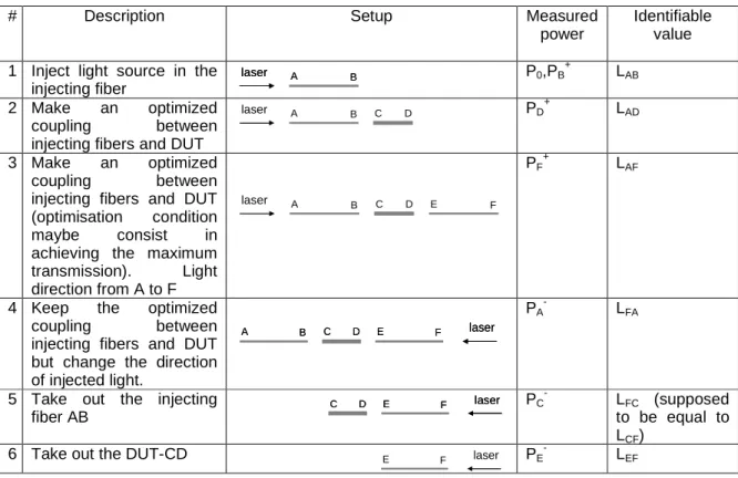
The procedure includes 6 steps detailed in Table 1. To measure the light power, an integrated sphere powermeter with suitable photodetector is used. Let us stress again that both the light source and the receiving section are maintained the same for the complete measurement procedure. Pk+ represents the measured power at point k when light direction
is from A to F. Pk- represents the measured power at point k when light direction is from F
to A. The light source is a laser diode which emits light with power of P0 at a specific
wavelength λ0.
Table 1. Different steps of measurement and associated identifiable values.
# Description Setup Measured
power
Identifiable value 1 Inject light source in the
injecting fiber A B F laser A B F laser P0,PB+ LAB 2 Make an optimized coupling between
injecting fibers and DUT
A B C D F laser PD + LAD 3 Make an optimized coupling between
injecting fibers and DUT (optimisation condition
maybe consist in
achieving the maximum transmission). Light direction from A to F
A B C D E F
laser
PF+ LAF
4 Keep the optimized
coupling between
injecting fibers and DUT but change the direction of injected light. A B C D E F laser A B C D E F laser PA - LFA
5 Take out the injecting
fiber AB E F C D E F laser C D laser PC - LFC (supposed to be equal to LCF)
6 Take out the DUT-CD
E F laser PE
-
In steps 1, 3, 4, 6 of the procedure, the connecting loss between laser and coupling fiber are included in the loss of the coupling fiber. It is straightforward to establish the 3 following equations with 3 variables (LBC, LCD, LDE):
LBC +LCD +LDE =LBE =LAF−LAB−LEF (1)
BC CD BD AD AB
L +L =L =L −L (2)
CD DE CE CF EF
L +L =L =L −L (3)
From (1) and (2), we find the coupling loss LDE =LAF −LEF −LAD. From (1) and (3), we find the coupling loss LBC =LAF−LAB−LCF. By replacing LDE and LBC in (1), we find the waveguide losses of the DUT LCD =LAF−LAB−LEF −LBC−LDE.
In the case where the DUT is an optical fiber, the procedure is straightforward. However, if the DUT is a waveguide with a length of some millimeters, the measurement of PD+ (step 2) and of PC- (step 5) can be inaccurate because the detector may collect not
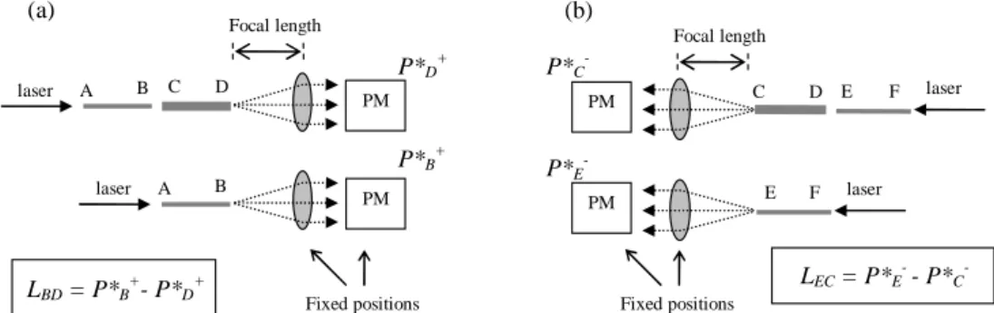
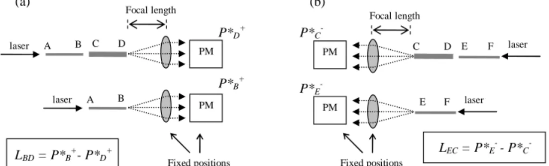
only the power at the waveguide output but also the power at the output of the coupling fiber which passes through the air (over and beneath the waveguide) because of very short length between coupling fiber and detector. To minimize this inaccuracy, the measurements in step 2 (and step 5) should be performed by two sub-steps with the help of an objective of microscope inserted in front of the detector at a fixed distance (see Figure 2). The optical objective is chosen so that its numerical aperture (NA) is large enough to be suitable with the NA of the DUT and of the coupling fibers. The power measured with the detector through the objective is presented with a star mark. In order to get rid of the losses due to the additional objective, we identify LBD instead of LAD (step 2) and LEC instead of LFC (step
5). The value of LBD (and LEC) is obtained by means of the two previously described sub
steps where P*D+ and P*B+ (P*C- and P*E- respectively) are measured. The rest of the
procedure is unchanged compared with the case where the DUT is an optical fiber.
(a) A B C D laser Fixed positions Focal length PM LBD = P*B+- P*D+ P*B+ P*D+ A B laser PM E F C D laser Focal length LEC = P*E-- P*C -P*C- P*E- (b) PM E F laser PM Fixed positions
Fig. 2. Setup of measurements in step 2 (a) and in step 5 (b) when the DUT is a waveguide. PM: powermeter.
Let us notice that if cladding, weakly guiding and/or radiation modes exist in the waveguide they will not be measured with the objective. So they will influence only the waveguide losses but not the coupling losses.
3. Experiments
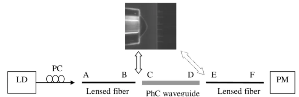
3.1 DUT is a waveguide
The experimental setup is shown in Figure 3. The DUT is a photonic crystal (PhC) waveguide fabricated in the framework of the COPERNICUS project by Thales Research and Technology [14]. The waveguide is 1.3 mm long, butted at extremities by inverse tapers. The inverse taper enlarges the mode field diameter of the waveguide up to 1.35 µm. The coupling fibers are micro-lensed fibers, named Gradhyp, fabricated by Foton laboratory [15]. The MFDs of these micro-lensed fibers are 2.7±0.1 µm (measured at
2
1/ e of maximum intensity) and the working distance is 28 µm. The NA of the objective used in the power measurements is 0.95. To maintain the injected polarization state during the whole measurement procedure, a polarisation controller is needed in the measurement set-up. Results of measurements for each step are summarised in Table 2.
LD PM
PhC waveguide Lensed fiber Lensed fiber
PC
A B C D E F
Fig. 3. Experimental setup of loss measurement in waveguides. PC: polarisation controller; LD: Laser diode; PM: powermeter.
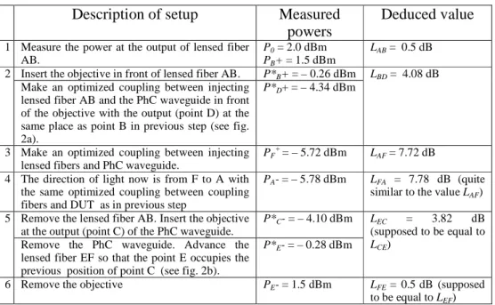
Table 2. Measurements and associated calculated losses.
Description of setup Measured powers
Deduced value
1 Measure the power at the output of lensed fiber AB.
P0 = 2.0 dBm
PB+ = 1.5 dBm
LAB = 0.5 dB
Insert the objective in front of lensed fiber AB. P*B+ = – 0.26 dBm
2
Make an optimized coupling between injecting lensed fiber AB and the PhC waveguide in front of the objective with the output (point D) at the same place as point B in previous step (see fig. 2a).
P*D+ = – 4.34 dBm
LBD = 4.08 dB
3 Make an optimized coupling between injecting lensed fibers and PhC waveguide.
PF+= – 5.72 dBm LAF = 7.72 dB
4 The direction of light now is from F to A with the same optimized coupling between coupling fibers and DUT as in previous step
PA- = – 5.78 dBm LFA = 7.78 dB (quite
similar to the value LAF)
Remove the lensed fiber AB. Insert the objective at the output (point C) of the PhC waveguide.
P*C- = – 4.10 dBm
5
Remove the PhC waveguide. Advance the lensed fiber EF so that the point E occupies the previous position of point C (see fig. 2b).
P*E- = – 0.28 dBm
LEC = 3.82 dB
(supposed to be equal to LCE)
6 Remove the objective PE- = 1.5 dBm LFE = 0.5dB (supposed
By replacing all the above values into (1), (2) and (3) and by considering that LCE =LEC, we have: 7.72 0.5 0.5 6.72 BC CD DE L +L +L = − − = (4) 4.08 BC CD L +L = (5) 3.82 CD DE L +L = (6)
By solving (4), (5), and (6), we obtain LDE = 2.64 dB which corresponds to the input
coupling loss, LBC = 2.90 dB (output coupling loss) and LCD = 1.18 dB (waveguide losses).
In the results, we observe that the coupling loss are slightly dissimilar, this is because the two microlenses used on both sides are not exactly the same. In fact the transverse mode field intensity profile of one of them is slightly elliptical, with a mode field diameter of 2.65 µm and 2.75 µm in horizontal and vertical axis respectively and the second one is circular with 2.7 µm of mode field diameter. Moreover the tapers may also be weakly different on both sides of the device.
Let us notice that we use only LAF in the calculation and not LFA (slightly different from
LAF in our case) because we consider Lij=Lji. The fact that LAF is different from LFA can be
explained by the fact that Lij is different from Lji somewhere in the system. In our concrete
case we think that this difference mainly comes from the DUT which contains tapers. So we can conclude that LCD would be different from LDC in an amount of 0.06 dB (ie LAF
-LFA).
Waveguide losses include linear, waveguide to taper transition and backscattering losses. Therefore, the identification of linear losses is not easy as all the other contributions should be subtracted from the computation. However, this term can be considered as dominant in our case. In fact, if we suppose that only linear losses contribute to power attenuation in the 1.3 mm waveguide, the average waveguide losses per unit length are 0.91 dB/mm, which is quite close to the simulated value of 10 dB/cm announced in [16].
Coupling losses on the contrary could be computed by means of the exact coupling efficiency calculation illustrated in [4]. However in our case, where the two circular gaussian modes are assumed to be well aligned, the estimation formula described in [17] can be used to evaluate the coupling efficiency η between two beams with mode field radii ω1 and ω2 respectively through 2 2
(
2 2)
21 2 1 2
4
η= ω ω ω ω+ . With the value ω1 = 1.35 µm for the mode field radius of the coupling fiber and ω2 = 0.64 µm for the mode field radius of the PhC waveguide (measured by near field technique), the coupling efficiency is η = 0.6 which leads to 2.2 dB of loss per facet instead of 2.64 dB and 2.90 dB (measured values at the input and output facet respectively). The difference between the estimated and the measured values can be explained by considering the addition of reflection losses on the fibres and tapers extremities, the non-perfect gaussian mode profile at the output of the taper [17], the misalignments of modes, etc.
3.2 DUT is an optical fiber with no connector at its ends
We also performed the measurements with a nonlinear microstructured holey silica fiber (355 meter long, without connectors). For injecting fibers, we use two high numerical aperture fibers with mode field radii of 1.78 µ m. The setup is similar to Figure 3. The measurement results are presented in Table 3.
Table 3. Power measurements (dBm) for microstructured holey silica fiber.
P0 PF+ PD+ PB+ PA- PC- PE-
0.80 –13.08 –9.25 0.10 –13.06 –9.08 0.49
From these measurements, coupling and linear losses are then deduced to be 3.30 dB for LBC, at the input, 3.52 dB for LDE at the output and 6.05 dB for linear loss LCD (i.e. 17.04
dB/km). By cutback method, we found linear loss of 6.20 dB (i.e 17.46 dB/km) which is about 2 % different in comparison with the results given by our method. As concerns the high values of coupling loss, we attribute it mainly to the very small size of the microstructured holey silica fiber (mode field radius is of 0.8 µm, measured by far field method). Using the theoretical equation of coupling efficiency [17], considering perfect circular Gaussian beams and perfect alignment, we obtained an estimated loss of 2.54 dB instead of 3.30 and 3.52 dB for measured coupling losses. This difference can be attributed again to non perfect Gaussian beam as we noticed, and could also be due to misalignment in angle and fiber positions.
4. Discussion
We note that during the measurements, the coupling does not need to be minimized but it must be optimized so that it is unchanged through steps in the procedure. Another point is that, if the DUT is polarisation-dependent, a polarisation controller must be used at the output of the laser and the state of polarisation of the signal injected into the DUT must remain unchanged in the case of forward injection as well as in the case of backward injection.
Concerning the error of the measurements, we notice that each power measurement task can be read with an error of ±0.01 dB which leads to a maximum for all of the deduced losses in our calculation of ±0.08 dB (corresponding to a calculation from 8 power values).
When DUT is a waveguide, the measurements of LBD and LEC can be performed with
the help of a CCD camera (instead of a powermeter) because each value can be deduced as relative integrated intensity values from two images measured in the two sub-steps. We have re-performed the measurements with the same waveguide in section 3 by using a camera. Losses in the waveguide were found to be 1.2 dB which is only 4 % different from the previous measured value. Let us notice again that the waveguide losses include all losses in the waveguide comprising linear losses and any reflection or scattering losses.
5. Conclusion
We have presented a new method for waveguide and coupling losses measurement between coupling fibers and single-mode optical guiding structures including fibers and waveguides with no connector at its ends. The method is non-destructive and there is no limitation of the length of the device under test. Several performed measurements with good results demonstrate the validity of the method.
Acknowledgement
The authors would like to thank Photonics Bretagne in Lannion for lending the microstructured holey silica fiber and the support of the EU through the Copernicus project (249012) (www.copernicusproject.eu) and Michel Gadonna from Foton for fruitful discussions.
References and links
1. G. P. Agrawal, in Fiber Optic Communication Systems, 3rd ed., (Wiley, New York, 2002).
2. R. Hui and M. O’Sullivan, in Optical fiber measurement, (Elsevier Academic Press, 2009).
3. Tachikura, Masao, "Internal Loss Measurement Technique for Optical Devices Equipped with Fiber Connectors at Both Ends," Applied Optics, 34, 8056-8057 (1995). 4. R. G. Hunsperger, in Integrated Optics: Theory and Technology, 3rd ed. (Springer
Verlag, New York, 1991).
5. H.P. Weber et al., “Loss measurements in thin film optical waveguides,” Appl. Opt.,
12(4), 755-757 (1973).
6. Y. Okamura, S . Yoshinaka, and S. Yamamoto, “Observation of wave propagation in integrated optical circuits,” Appl. Opt., 25(19), 3405-3408 (1986).
7. R. K. Hickemell et al., “Waveguide loss measurement using photothermal deflection,” Appl. Opt., 27(13), 2636-2638 (1988).
8. R. Arsenault, D. Gregoris, S . Woolven, V.M. Ristic, “Waveguide propagation-loss measurement technique,” Opt. Lett., 12(12), 1047-1049 (1987).
9. R. G. Walker, ‘‘Simple and accurate loss measurement technique for semiconductor optical waveguide,” Electron. Lett., 21(13), 581-583 (1985).
10.R. Regener and W. Sohler, “Loss in low-finesse Ti:LiNbO3 optical waveguide resonators,” Appl. Phys. B., 36(3), 143-147 (1985).
11.T. Feuchter and C. Thirstrup, “High Precision Planar Waveguide Propagation Loss Measurement Technique Using a Fabry-Perot Cavity,” IEEE Photon. Techn. Letters,
6(10), 1244-1247 (1994).
12.W. B. Joyce and B. C. Deloach, “Alignment of Gaussian beams”, Appl. Opt. 23, (23), 4187-4196, (1984).
13.L. Jaroszewicz et al. “Low-Loss Patch Cords by Effective Splicing of Various Photonic Crystal Fibers with Standard Single Mode Fiber”, JLT, 29 (19), pp. 2940 - 2946 (2011). 14.Q. V. Tran, S. Combrié, P. Colman, and A. De Rossi, “Photonic crystal membrane
15.M. Thual, P. Rochard, P. Chanclou, and L. Quetel, “Contribution to research on Micro-Lensed Fibers for Modes Coupling”, Fiber and Integrated Optics, 27(6), 532-541 (2008).
16.S. Combrié, E. Weidner, A. DeRossi, S. Bansropun, and S. Cassette, “Detailed analysis by Fabry-Perot method of slab photonic crystal line-defect waveguides and cavities in aluminium-free material system,” Opt. Express, 14(16), 7353-7361 (2006).
17.J-I Sakai and T. Kimura, “Design of a miniature Lens for Semiconductor Laser to Single-Mode Fiber Coupling, IEEE J. Quant. Electron., 16(10), 1059-1066 (1980). 18.A. Akrout, K. Lengle, T. N. Nguyen, P. Rochard, L. Bramerie, M. Gay, M. Thual, S.
Malaguti, A. Armaroli, G. Bellanca, S. Trillo, S. Combrié, A. De Rossi, “Coupling between PhC membrane and lensed fiber : simulations and measurements”, TuD5, Rome, Italy, NUSOD (2011).
Figures :
A B C D E F
LAB LBC LCD LDE LEF laser
Fig. 1. Principle of loss measurement technique.
(a) A B C D laser Fixed positions Focal length PM LBD = P*B+- P*D+ P*B+ P*D+ A B laser PM E F C D laser Focal length LEC = P*E-- P*C -P*C- P*E- (b) PM E F laser PM Fixed positions
Fig. 2. Setup of measurements in step 2 (a) and in step 5 (b) when the DUT is a waveguide. PM: powermeter.
LD PM
PhC waveguide Lensed fiber Lensed fiber
PC
A B C D E F
Fig. 3. Experimental setup of loss measurement in waveguides. PC: polarisation controller; LD: Laser diode; PM: powermeter.
Table 1. Different steps of measurement and associated identifiable values.
# Description Setup Measured
power
Identifiable value 1 Inject light source in the
injecting fiber A B F laser A B F laser P0,PB + LAB 2 Make an optimized coupling between
injecting fibers and DUT
A B C D F
laser PD+ LAD
3 Make an optimized
coupling between
injecting fibers and DUT (optimisation condition
maybe consist in
achieving the maximum transmission). Light direction from A to F A B C D E F laser PF + LAF
4 Keep the optimized
coupling between
injecting fibers and DUT but change the direction of injected light.
A B C D E F laser
A B C D E F laser
PA- LFA
5 Take out the injecting
fiber AB E F C D E F laser C D laser PC - LFC (supposed to be equal to LCF)
6 Take out the DUT-CD
E F laser PE
- L
Table 2. Measurements and associated calculated losses.
Description of setup Measured powers
Deduced value
1 Measure the power at the output of lensed fiber AB.
P0 = 2.0 dBm
PB+ = 1.5 dBm
LAB = 0.5 dB
Insert the objective in front of lensed fiber AB. P*B+ = – 0.26 dBm
2
Make an optimized coupling between injecting lensed fiber AB and the PhC waveguide in front of the objective with the output (point D) at the same place as point B in previous step (see fig. 2a).
P*D+ = – 4.34 dBm
LBD = 4.08 dB
3 Make an optimized coupling between injecting lensed fibers and PhC waveguide.
PF +
= – 5.72 dBm LAF = 7.72 dB
4 The direction of light now is from F to A with the same optimized coupling between coupling fibers and DUT as in previous step
PA- = – 5.78 dBm LFA = 7.78 dB (quite
similar to the value LAF)
Remove the lensed fiber AB. Insert the objective at the output (point C) of the PhC waveguide.
P*C- = – 4.10 dBm
5
Remove the PhC waveguide. Advance the lensed fiber EF so that the point E occupies the previous position of point C (see fig. 2b).
P*E- = – 0.28 dBm
LEC = 3.82 dB
(supposed to be equal to LCE)
6 Remove the objective PE- = 1.5 dBm LFE = 0.5dB (supposed
to be equal to LEF)
Table 3. Power measurements (dBm) for microstructured holey silica fiber.
P0 PF+ PD+ PB+ PA- PC- PE-