Fast semi-automatic segmentation algorithm for Self-Organizing Maps

HAL Id: hal-00435732

https://hal.archives-ouvertes.fr/hal-00435732

Submitted on 24 Nov 2009

HAL is a multi-disciplinary open access

archive for the deposit and dissemination of

sci-entific research documents, whether they are

pub-lished or not. The documents may come from

teaching and research institutions in France or

abroad, or from public or private research centers.

L’archive ouverte pluridisciplinaire HAL, est

destinée au dépôt et à la diffusion de documents

scientifiques de niveau recherche, publiés ou non,

émanant des établissements d’enseignement et de

recherche français ou étrangers, des laboratoires

publics ou privés.

Fast semi-automatic segmentation algorithm for

Self-Organizing Maps

David Opolon, Fabien Moutarde

To cite this version:

David Opolon, Fabien Moutarde. Fast semi-automatic segmentation algorithm for Self-Organizing

Maps. European Symposium on Artifical Neural Networks (ESANN’2004), Apr 2004, Bruges,

Bel-gium. �hal-00435732�

Fast semi-automatic segmentation algorithm

for Self-Organizing Maps

David Opolon and Fabien Moutarde

Ecole des Mines de Paris, 60 bd Saint-Michel, F-75272 Paris Cedex 06, France.

Abstract. Self-Organizing Maps (SOM) are very powerful tools for data

mining, in particular for visualizing the distribution of the data in very high-dimensional data sets. Moreover, the 2D map produced by SOM can be used for unsupervised partitioning of the original data set into categories, provided that this map is somehow adequately segmented in clusters. This is usually done either manually by visual inspection, or by applying a classical clustering technique (such as agglomerative clustering) to the set of prototypes corresponding to the map.

In this paper, we present a new approach for the segmentation of Self-Organizing Maps after training, which is both very simple and efficient. Our algorithm is based on a post-processing of the U-matrix (the matrix of distances between adjacent map units), which is directly derived from an elementary image-processing technique. It is shown on some simulated data sets that our partitioning algorithm appears to give very good results in terms of segmentation quality. Preliminary results on a real data set also seem to indicate that our algorithm can produce meaningful clusters on real data.

1.

Introduction

Self-Organizing Maps (SOM, invented by T. Kohonen in 1981 [7, 8]) have turned out to be very powerful for gaining insight into data repartition [5, 10, 12]. Indeed, SOM can provide a very valuable human-interpretable visualization of the distribution of very high dimensional data: it determines a set of prototypes that represent the data, and are organized in a way that achieves a topology-preserving projection from the data space onto a low-dimensional space (generally a 2D grid). This grid provides a useful and directly interpretable view of some characteristics of the analyzed data set, in particular its cluster structure [15, 16].

Moreover, SOM can be used not only as a powerful data set visual inspection device, but as a tool for partitioning the data into categories (i.e. identifying separate clusters in the input space). This is theoretically quite simple to do: visual identification of groups of prototypes on the obtained map is fairly easy, and it is then absolutely straightforward to deduce a partitioning of the data set from the determined clusters of prototypes. One of the advantages of using SOM segmentation for clustering is that no a priori hypothesis on the number of clusters is required. However, it is highly desirable to automate the segmentation of the map into clusters instead of having to rely on a visual and manual definition of the groups of prototypes.

Vesanto and Alhoniemi [14] proposed and used with some success the application of classical hierarchical agglomerative and partitive clustering techniques to the SOM prototypes. As pointed out in [14], this approach allows to reduce significantly the computation time as compared to applying the clustering algorithm directly to the original data, since the number of prototypes is the size of the map, which is normally much less than the number of data points. F. Murtagh [9] has proposed an even more efficient variant, which consists in applying a contiguity-constrained clustering algorithm, taking thus advantage of the neighborhood relations between map units. Nevertheless, all these techniques require the computation of a significant number of within-cluster or inter-cluster distances (for a complexity analysis, see for instance [3]), whose computation cost is also proportional to the dimension of the input data. This could become problematic when applied to very high dimensional data such as those used in text-mining (see [11]).

In this paper, we propose an alternative technique for segmenting Self-Organizing Maps, which is both very simple and efficient. Our algorithm also takes full advantage of the neighborhood relations between prototypes by computing only the distances between neighboring prototypes (and by computing them only once).

2.

The Algorithm

The basic idea of our SOM segmentation algorithm is to apply a simple area-filling algorithm to the U-matrix of the SOM (i.e. the matrix of distances between adjacent map units [12]). More precisely, for every prototype pi,j of the SOM (placed at the (i,j)

position on the SOM grid), we first compute the two following distances:

•

(

)

•

(

)

where dist(pi,j , pn,m) is the euclidian distance in input space between pi,j and pn,m.

The initial variant of our algorithm considers only the mean distance of each prototype pi,j to its four neighbors on the map pi-1,j, pi+1,j, pi,j-1, and pi,j+1:

(

)

,j i j i j i j i j

i eastDist eastDist southDist southDist

meanDist = ₋ + + ₋ +

We then determine the frontiers of each visually-identified cluster Ck on the SOM

grid with the following region-growing algorithm, directly adapted from standard area-filling techniques:

- define a threshold distance dmink for cluster Ck

- start from any prototype pi0,j0 which is clearly inside the cluster Ck

- apply to (i0,j0, dmink, k) the following recursive procedure:

floodFillMoy(i, j, dmink, k) {

if (i,j) is inside the SOM grid range, then:

if (pi,j is not tagged as member of Ck) and (meanDisti,j < dmink), then do:

- tag pi,j as member of Ck - floodFillMoy(i+1,j,dmink,k)

- floodFillMoy(i-1,j,dmink,k)

- floodFillMoy(i,j-1,dmink,k)

- floodFillMoy(i,j+1,dmink,k)

3.

Experiments and results on artificial data sets

We conducted various tests on simulated data sets for which the desired result of the clustering was obvious. Some of them contained several very well separated convex clusters of points (such as the one presented on left of fig.1). Others were more sophisticated clustering benchmarks such as the "chain link" example proposed by [13], which consists of two intertwined 3D rings (see right of fig.1).

Figure 1: An example of 2D simulated data set (left), and an example of 3D simulated data set, consisting of two 3D rings intertwined as a chain link (left).

For the SOM algorithm, we used a gaussian kernel neighborhood and a linearly decreasing learning rate. After the algorithm has converged, we compute the U-matrix of the map, and visualize the "mean distance to neighbors" as defined in §2 (see left of figures 2 and 3). Then we apply our region-growing algorithm separately to each visually-identified cluster, using for each of them a different threshold chosen as the maximum possible value that does not induce a propagation to other clusters. We thus obtain a segmentation of the map, where each region is separated from the others by some "no man's land" (or "frontier") units (see figures 2 and 3).

Figure 2: Visualization of the typical "mean distance to neighbors" matrix for the SOM obtained on the 2D data set of fig.1 (left). Corresponding segmentation of the SOM produced by our algorithm (middle). Clustering result (right): no points are affected to the wrong cluster,

and only a few "border" points end up unclassified (big stars).

Once the segmentation is done, we attribute a particular label to each region of the map, and simply tag every original data point with the label of its best matching unit (BMU). Of course, since some units do not belong to any region, any data point whose BMU is a frontier unit will have a specific "unclassified" tag. We then analyze the labeled data points, in order to assess the quality of the obtained clustering. In our tests, there was nearly never any misclassification, i.e. nearly no data point was erroneously labeled as part of a cluster it does not belong to. However, as expected, some data points were left "unclassified", but there were very few of them and most were on the border of the clusters, as illustrated on the rightmost part of figure 2.

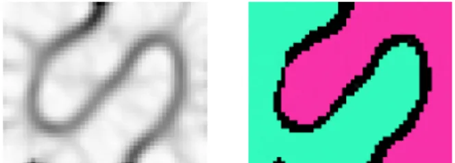
Figure 3: Visualization of the typical “U-matrix” for the SOM obtained on the "chain link" 3D data set (left), and corresponding segmentation of the SOM produced by our algorithm (right).

For our experiments on the "chain link" data set, 100% of the points were classified in the correct cluster. For the 2D data set presented on figures 1 and 2, there was usually no misclassified points, and the typical number of "unclassified" points was 20 to 30 on a total of 2000, which is a very small proportion (1% or 2%).

4.

Preliminary results on real data sets

In order to evaluate if our algorithm produces meaningful clusters on real data sets, we began to try it on a few of them. We first used the famous Fisher’s iris data set [4]. This real 4-dimensional data set contains 50 examples for each of 3 iris flower classes. It is a very popular benchmark for classification and clustering techniques.

Depending on the SOM parameters used, we obtained between 2 and 4 clusters. One of the clusters always nearly coincided with the Setosa iris species (which is linearly separable from the two other classes), and the others generally made sense as compared to the 3 iris categories (see examples in tables 1 and 2).

Cluster 1 Cluster 2 Cluster 3 Cluster 4 Outside clusters

Iris Setosa 49 0 0 0 1

Iris Versicolor 0 33 1 0 14

Iris Virginica 0 3 34 8 7

Table 1: Example of clustering obtained on the iris data set, each column showing the class membership distribution of the points of one of the produced clusters. Nearly all points of each

given cluster belong to the same iris class. However, 22 irises are outside all 4 clusters.

Cluster 1 Cluster 2 Cluster 3 Outside clusters

Iris Setosa 0 50 0 0

Iris Versicolor 27 0 1 22

Iris Virginica 6 0 35 9

Table 2: A second example of clustering obtained on the iris data set, in which the number of clusters is exactly the number of iris classes. However, cluster #1 significantly overlaps 2

different iris classes, and 31 irises do not belong to any of the 3 obtained clusters.

The global typical outcome of our algorithm on the iris data set compares favorably to partitions obtained, for instance, by Blatt et. al. with various other clustering methods (see [2]), or with those reported in [6] or in [1].

Other very preliminary tests conducted on bigger and more complex real data sets also seem encouraging, but require further analysis.

5.

Computational cost

As can be seen in [14], the computational cost of partitioning a SOM is not always negligible compared to that of the SOM training (especially when k-means clustering is used). Moreover, as pointed out in [3], standard hierarchical clustering techniques have an over-all computational complexity of at least O(n2_{logn) where n is the} number of elements to cluster. In the case of SOM segmentation, n is the number of units on the map, which is normally much lower than the original data set size N. However, since the complexity of SOM training is in O(n), it is clear that for a given data set size N, the relative computational cost of the segmentation increases quickly with the map size n. And when one wants to use the trained SOM for non-parametric clustering by a posteriori segmentation of the map, it is desirable to use relatively big maps (i.e. with n values of a few hundreds)… For the algorithm we propose here, it is straightforward to deduce from its description in §2 that it is in O(n), and that the essential cost is the computation of the 2*n adjacent unit distances required to obtain the U-matrix. Therefore, contrary to most SOM segmentation techniques, the computational cost of our partitioning procedure relative to that of the SOM training should always remain negligible, whatever the chosen grid size.

6.

Conclusion, discussion and perspectives

In this paper we presented a new algorithm for segmenting Self-Organizing Maps after training, in order to use the SOM as a clustering technique for the input data. Our algorithm, directly adapted from standard area-filling techniques, is extremely simple, but appears to produce very good clustering results, at least on the simulated data sets on which we tested it (see §3). Preliminary results a few real data sets are also encouraging, as illustrated in §4 on the case of Fisher's iris data set. Compared to usual SOM partitioning techniques, our algorithm also has the advantage to have an extremely low computational cost. It thus has the potential to be a powerful tool for automating the discovery of meaningful categories in big data sets.

More thorough tests on other and more complicated real data sets are necessary and currently underway. Also, one drawback of our SOM segmentation approach in its current form, is that the threshold value has to be manually determined by trial and error for each visually-identified cluster, making it semi-automatic rather than fully automated. However, we are currently improving our procedure in order to overcome this problem without impairing its computational efficiency. Another ongoing improvement consists in taking better advantage of the U-matrix by propagating the area-filling differently in each direction, by taking into account the vector of distances to adjacent units instead on simply relying on the mean distance to the four neighbors.

References

[1] A. Ben-Hur, D. Horn, H.T. Siegelmann, V. Vapnik: A support vector method for clustering, Advances in Neural Information Processing Systems 13, 367-373, 2001. [2] M. Blatt, S. Wiseman, E. Domany. Data clustering using a model granular magnet, Neural Computation, 9:1805-1842, 1997.

[3] M. Dash and H. Liu. Efficient hierarchical clustering algorithms using partially overlapping partitions. Lecture Notes in Computer Science, volume 2035, pp 495-507, 2001.

[4] R.A. Fisher. The use of multiple measurements in taxonomic problems. Annals of

Eugenics, 7:179 188, 1936.

[5] J. Himberg, J. Ahola, E. Alhoniemi, J. Vesanto and O. Simula. The Self-Organizing Map as a tool in knowledge engineering. Pattern Recognition in Soft

Computing Paradigm, chapter 1, 2001.

[6] A.L. Hsu and S.K. Halgamuge. An unsupervised hierarchical dynamic self-organizing approach to cancer class discovery and marker gene identification in microarray data (supplementary information on “Dynamic SOM with hexagonal structure for data mining”). Bioinformatics, Vol. 19(16), pp. 2131-2140, 2003

[7] T. Kohonen. Automatic formation of topological maps of patterns in a self-organizing system. Proceedings of 2nd Scandinavian Conference on Image Analysis

(SCIA) held in Helsinki (Finland), pages 214-220, 1981.

[8] T. Kohonen. Self-organizing formation of topologically correct feature maps.

Biological Cybernetics, 43(1):59-69, 1982.

[9] F. Murtagh. Interpreting the Kohonen self-organizing map using a contiguity-constrained clustering. Pattern Recognition Letters, vol. 16, pp 399-408, 1995. [10] S. Mitra, S.K. Pal and P. Mitra. Data mining in soft computing framework: a survey. IEEE Transactions on Neural Networks, volume 13(1), pages 3-14, 2002. [11] M. Steinbach and G. Karypis and V. Kumar. A comparison of document clustering techniques. KDD Workshop on Text Mining, 2000.

[12] A. Ultsch and H.P. Siemon. Kohonen's self organizing feature maps for exploratory data analysis. Proceedings of 1990 Int. Neural Network Conference

(INNC'90) held in Dordrecht (Netherlands), Kluwer, pages 305-308, 1990.

[13] A. Ultsch and C. Vetter. Self-Organizing-Feature-Maps versus statistical clustering methods: a benchmark. FG Neuroinformatik & Kuenstliche Intelligenz,

University of Marburg, Research Report 0994, 1994.

[14] J. Vesanto and E. Alhoniemi. Clustering of the Self-Organizing Map. IEEE

Transactions on Neural Networks, Volume 11(3), 2000.

[15] J. Vesanto. SOM-based data visualization methods. Intelligent Data Analysis, Volume 3(2), 1999.

[16] J. Vesanto. Using SOM in data mining. Licentiate thesis, Helsinki University of