HAL Id: hal-00640713
https://hal.archives-ouvertes.fr/hal-00640713
Submitted on 14 Nov 2011
HAL is a multi-disciplinary open access
archive for the deposit and dissemination of
sci-entific research documents, whether they are
pub-lished or not. The documents may come from
teaching and research institutions in France or
L’archive ouverte pluridisciplinaire HAL, est
destinée au dépôt et à la diffusion de documents
scientifiques de niveau recherche, publiés ou non,
émanant des établissements d’enseignement et de
recherche français ou étrangers, des laboratoires
telecommunications service providers
Patrick Maillé, Bruno Tuffin, Jean-Marc Vigne
To cite this version:
Patrick Maillé, Bruno Tuffin, Jean-Marc Vigne. Technological investment games among wireless
telecommunications service providers. Journal of Communications and Networks, IEEE & Korea
Information and Communications Society, 2011, 21 (1), pp.65-82. �10.1002/nem.776�. �hal-00640713�
Technological Investment Games Among Wireless
Telecommunications Service Providers
‡Patrick Maill´e
1, Bruno Tuffin
2and Jean-Marc Vigne
1,2 ∗†1Institut Telecom; Telecom Bretagne; 2, rue de la Chˆataigneraie CS 17607 35576 Cesson S´evign´e Cedex, France 2Dionysos team, INRIA Rennes - Bretagne Atlantique, Campus Universitaire de Beaulieu 35042 Rennes, France
SUMMARY
With the development of new technologies in a competitive context, infrastructure investment and licence purchase as well as existing technology maintenance are crucial questions for current and emerging operators. This paper presents a three-level game analyzing this problem. At the highest level, the operators decide on which technologies to invest, given that some may already own licences or infrastructures. We limit ourselves to the realistic case where technologies are 3G, WiFi and WiMAX. At the intermediate level, with that set of operated technologies fixed, operators determine their service price. Finally, at the lowest level, customers choose their provider depending on the best combination of price and available quality of service. At each level, the best decision of actors depends on the actions of others, the interactions hence requiring to be studied as a (noncooperative) game. The model is analyzed by backward induction, meaning that decisions at a level depend on the equilibria reached at the lower levels. Different real-life cost scenarios are studied. Our model aims at helping both the operators to make their final decision on technological investments, and the regulator to determine a proper licence fee range for a better competition among providers. Copyright © 2008 John Wiley & Sons, Ltd.
KEY WORDS: Network pricing, Nash equilibrium, Wardrop equilibrium, technological game, telecommunica-tion investments
1. INTRODUCTION
Telecommunications are becoming omnipresent, with all kinds of services, telephony, television, web browsing, email, etc., now available on the same terminals. Similarly, due to the market liberalization, customers may choose among different providers, their choice being based on different parameters such as price, quality of service (QoS), coverage or used technology for instance. Those providers are therefore competitors, fighting to attract customers in order to maximize their revenue. In this context, providers need to carefully determine not only the access price they will impose, but also on which set of technologies to operate. Basically when talking about wireless providers, the choice is among 3G, WiFi and WiMAX (or LTE).
∗Correspondence to: Jean-Marc Vigne, Telecom Bretagne, 2 rue de la Chˆataigneraie CS 17607 35576 Cesson-S´evign´e Cedex,
France
†Email: [email protected]
We will assume in this paper that customers have at their disposal terminals supporting multiple interfaces, and the technology used is the one providing the best combination of price and QoS meaning that there is no coverage issue (all technologies can be potentially used by all customers). Our goal is to model, understand and propose to operators strategical choices in terms of technology investment, as well as to suggest rules that a regulator could apply to induce a more efficient competition (from a global or a user perspective). Examples of questions we aim at answering are:
• is it worth for an operator paying a licence and an infrastructure for being present in a new technology? Will the return on investment be sufficient? That question is typical of what operators ask themselves with regard to the implementation of WiMAX [2] or LTE.
• Does this investment help to attract more customers, or is it just at the expense of other technologies already implemented? This has to be studied in a competitive environment, given that other operators may make similar strategic moves. Some operators may already be present on some technologies, and therefore their costs are limited; this potential heterogeneity has also to be taken into account.
• Why investing on a technology where a competitor is installed and dominant? The total cost has to be pondered with the revenue from customers. A regulator, in order to break such dominant positions, may decide to compensate that unbalance through the licence fees. An illustration comes from the third generation wireless licences in France, where the regulator wants to open an additional licence to increase competition, this new licence being offered at a lower cost than the initial ones. Our paper helps understanding the range of licence fees allowing a candidate to enter the market and make benefits.
We introduce a model made of three levels of game, corresponding to three different time scales. At the lowest level, given fixed operated technologies and service costs, customers spread themselves among available operators in order to get the “best” combination of price and QoS, where the QoS (or the congestion) they get depends on the choice of the other users. To simplify the analysis, users are assumed infinitesimal. As a consequence, the (selfish) decision of a single individual does not have any influence on the system behavior. The equilibrium analysis is therefore provided by the so-called Wardrop’s principle [3] coming from transportation theory: at equilibrium, all providers with a positive demand have the same perceived combination of price and QoS, otherwise customers would switch to the “best”. When choosing their price at the intermediate level, providers can anticipate what the resulting equilibrium (and therefore their revenue) would be for a given price profile, i.e., for given and fixed prices for all providers, which induces a pricing game among providers at this second level. The general framework is here again that of non-cooperative game theory, and the equilibrium notion is now that of Nash equilibrium with atomic players [4]. Finally, at the largest time scale, providers can decide which technologies to operate. In order to make that decision, they have to compute what their revenue would be at the equilibrium or equilibria (if any) of the lower-level pricing game, and compare it with their costs. That choice, which also depends on the strategy of competitors, will be made in order to reach again a Nash equilibrium for this “technology game”. While there exist papers on the first two levels of game (see the literature review subsection below), we are not aware of any other paper analyzing the technological game, especially when using the results of the two other levels. This paper seems to be the first in that important direction of modeling and understanding the complete chain of provider strategies. We additionally illustrate the interest of our methodology by modeling practical situations of competition and technology investment arising in France.
1.1. Literature review
Several papers can be found on the two lower levels of game, i.e., the game among users to find the best provider and the pricing game among providers [5,6,7,8,9,10]. In [5], Acemoglu and Ozdaglar consider infinitesimal users choosing a provider so as to minimize their perceived price, that is the sum of a congestion cost and a financial charge. When an equilibrium on prices exists (and the authors show it does when congestion costs are linear), then competition is proved to lead to an overall social welfare not too far from the optimal one. Our model can be seen as a variation of theirs, by considering some technologies where the resource is shared among operators, and imposing operators to set a unique price for all the technologies they implement. The main extension though comes from the third level of game where providers can choose the operated technologies, and from the associated real-life scenarios. Another model in [6] describes several retailers periodically selling product units and competing on the initial fill rate (i.e., the fraction of available items to be sold), the periodical retail price and the stock-policy they choose. The authors show that an equilibrium on those parameters can be deduced from another equilibrium of a single-period game on prices and fill rates only. For some demand expressions, it is also shown that such equilibria exist. In our context, product units can be interpreted as data units or packets, and fill rates are supposed constant. Our model makes use of Wardrop principle to define the customer equilibrium, while attraction models are considered in [6]; above all, no technological game is considered there due to the different focus.
A model for the two lower levels of game has been again proposed in [7,8], similarly to ours; but congestion is modeled there by losses instead of delay, and the higher-level technological game is still not considered. In [10], a two-sided competition model is proposed. Users choose operators offering the highest utility in term of price and QoS too, but two populations, with different sensitivity to the two parameters are considered. Providers offer different QoS because they operate on different frequency bands, an aspect which can be covered by our model. A new aspect is that some bandwidth can be sold to ad-hoc networks, serving as secondary users. The equilibrium on prices is searched numerically by means of a learning algorithm, but there again, no technological game is considered.
There is to our knowledge no other paper dealing with the technology game, especially using the result of the pricing game. But other multilevel games exist, the most notable ones being [11] and [12]. Though, [11] rather models the interactions among Internet service providers and content providers, while we rather aim at investigating which technologies a provider should implement, given the potential revenue and the potential infrastructure and licence costs. On the other hand, [12] considers investments to improve the quality of service, but not to implement a new technology. Moreover, that paper mixes the investment and the pricing decisions into a single game level, while we separate here those choices due to different time scales. We have not seen elsewhere that kind of study in a similar competitive context. We also provide typical and real-life competition situations of providers already installed but which could try to extend their technological range to increase their revenue.
1.2. Organization
This paper is organized as follows. In Section2, we present the basic model that will be used: the user behavior, the set of providers and available technologies, and the three levels of game. The lowest level of game, that is the competition among users looking for the network with the best combination of price and QoS, is analyzed in Section3; the equilibrium is characterized, and existence and uniqueness are discussed. Section4analyzes the pricing game for fixed technologies, anticipating what the reaction of users would be. The third level of game, the game on technologies, is described in Section5. This game makes use of the revenues at the pricing-game level, and pastes the infrastructure and licence
costs. We show how this can be solved. Section6on the other hand considers practical situations of competition, and illustrates which equilibria can be found. Real-life scenarios are considered, typical of competition encountered in France, and we show how the model can help to propose relevant technological investment strategies for providers, but also to propose ranges of licence costs for the regulators towards a better use or sharing of the resource. We finally conclude and give directions for future research activities in Section7.
2. THE MODEL
We describe in this section the definitions and assumptions on the model, as well as the three levels of game that will be analyzed later on. We assume that we have a setN = {1, ..., N} of telecommunication providers trying to maximize their revenue. Each provider i∈ N has to decide which set of technologies Si it will operate, and the access price pi per unit of flow that a customer needs to pay if using her
network. The set of technologiesSi is to be chosen within a setT of available technologies. In our
practical scenarii, considering wireless operators, this set will be T = {3G, WiMAX, WiFi}.
This setT of technologies is partitioned into two subsets Tp andTs. For a technology in Tp, each
operating provider owns a licence and a part of the radio spectrum, using it alone. In other words, congestion on this technology depends only on the level of demand the operator experiences on her own network. On the other hand, for a technology inTs, the spectrum is shared by the customers of the
competing providers, so that congestion depends not only on the level of demand at the provider, but also on demand coming from competitors using this technology. Basically, we will consider
Tp= {3G, WiMAX} and Ts= {WiFi}.
We assume that the price pi charged by provider i ∈ N is independent of the technology used
by customers. In other words, provider i fixes a price for network access that is the same for all the technologies she operates. We moreover assume that users have terminals with multiple interfaces, allowing them to use any technology, and that they can sense the available QoS. The choice of the technology is left to the user terminal, that will (selfishly) choose a couple (provider, technology) offering the best combination of price and QoS.
Users are modeled by the aggregate level of flow demand di,texperienced at technology t∈ T by
provider i∈ N . Users are seen as infinitesimal (also said non-atomic), so that the action of a single user is considered having no impact, contrary to that of an (infinite) set of users. This kind of assumption is usual in the related transportation theory where a car has no influence on congestion, but where a flow of cars rather has to be dealt with. We call d the vector of all flow demands.
QoS is modeled by a congestion cost function ℓi,t of di,t for owned-spectrum technology t (i.e.,
t ∈ Tp) operated by provider i, and ℓtof total demand∑jdj,tfor shared-spectrum technology t (i.e.,
t ∈ Ts). Those functions are assumed strictly increasing -more demand implies more congestion-,
continuous and non-negative.
User behavior is modeled in the following way. We assume that each user tries to minimize her
perceived price ¯pi,t, that is for technology t and provider i defined by
¯ pi,t(d) = ⎧⎪⎪⎪⎪ ⎪⎨ ⎪⎪⎪⎪⎪ ⎩ pi+ ℓi,t(di,t) if t ∈ Tp pi+ ℓt ⎛ ⎝∑j dj,t ⎞ ⎠ if t∈ Ts. (1)
This means that the perceived price is a linear combination of a monetary cost (the price charged) and a QoS cost (the congestion level). Any other combination form could be considered, but we follow here the representation proposed in [5,13]. Our model is actually an extension of the one in [13], where
i)different technologies can be operated by a single provider, and ii) some can also be shared. This addition is for introducing the technological game which is not addressed in [5,13]. We will see in the next section how demand is distributed at equilibrium, which will result in a system perceived price ¯p, common to all technologies that do get some demand.
We also assume that total user demand d = ∑Ni=1∑t∈Sidi,t is a continuous function D(⋅) of the perceived price ¯p, strictly decreasing on its support and with limp→∞D(p) = 0. D(p) represents
the total amount of traffic that users would want to transmit at a fixed perceived unit price p, it may encompass (cumulated) individual demand variations with respect to price, and/or (cumulated) individual decisions to abandon the service. In addition, we call v the inverse function of D on its support.
The system is characterized by three different time scales, resulting in three different levels of game: • at the shortest time scale, for fixed prices and sets of offered technologies, users choose their provider and technology in order to minimize their perceived price. This drives to a user equilibrium situation(d∗i,t)i,t where for all technologies with positive demand, the perceived
price is the same, other technologies having larger perceived prices (otherwise some users would have an interest to change to a cheaper option).
• At the intermediate time scale, providers compete for customers by playing with prices for fixed sets of implemented technologies. The goal of each provider i is to maximize her revenue
Ri= ∑
t∈Si
pid∗i,t, (2)
playing on price pi and making use of what the user equilibrium d∗ = (d∗i,t)i,twould be for a
given price profile. Since the revenue of a provider depends on the price strategy of competitors (through the user equilibrium), this is analyzed using non-cooperative game theory.
• At the larger time scale, providers have to choose which technologies to invest on. This is again analyzed thanks to non-cooperative game theory, using the equilibrium situation(p∗i)1≤i≤N of
the intermediate level.The goal is here again to optimize
Bi= ∑
t∈Si (p∗
id∗i,t− ci,t)
(where ci,trepresents the licence and infrastructure costs to provider i to operate on technology
t), by playing with the setSi.
3. FIRST LEVEL OF GAME: COMPETITION AMONG USERS
To study our three-level game, we first need to determine how user demand is distributed among providers. Access prices are assumed fixed in this section, those prices only being changed at a larger time scale. Following our non-atomicity assumption about users, the equilibrium is driven by Wardrop’s principle [3] coming from transportation theory: at a user equilibrium the perceived price at each provider getting some demand is the same, otherwise, if one is larger than another, then her customers would prefer to change and go to the cheapest. Some providers may also be too expensive, with an access price larger than the perceived price of competitors, and therefore get no demand.
Wardrop’s principle can be formalized as follows. Consider a technology configuration S = (S1, ...,SN) and a price configuration (p1, ..., pN). A Wardrop (or user) equilibrium is a family
(di,t)i∈N ,i∈Siof positive real numbers such that ⎧⎪⎪⎪⎪ ⎪⎪⎪⎪⎪ ⎪⎪⎪ ⎨⎪⎪⎪ ⎪⎪⎪⎪⎪ ⎪⎪⎪⎪ ⎩ ∀i∈ N , ∀t ∈ Si p¯i,t=⎧⎪⎪⎪⎨⎪⎪⎪ ⎩ pi+ℓi,t(d∗i,t) if t ∈ Tp pi+ℓt( ∑ j∶t∈Sj d∗j,t) if t ∈ Ts
∀i∈ N , ∀t ∈ Si d∗i,t> 0 Ô⇒ ¯pi,t= min j∈N ,τ ∈Sj(¯p j,τ) ∑ i∈Nt∈S∑i d∗i,t= D( min i∈N ,t∈Si(¯p i,t)). (3)
The first equality presents the perceived price at each couple (operator, technology), separating the case where the technology is owned by the operator (inTp) and the case where it is shared (inTs). The
second equality states that users choose the cheapest option in terms of perceived price, and that the perceived price at providers getting demand is necessarily the same - otherwise, again, some customers would have an interest in churning - . Finally, the last equality states that total demand, i.e., sum of demands at each network, is the demand function at the perceived price.
Remark that this kind of nonatomic game played among users falls into the widely-studied set of routing games [14,15,16]. Indeed, the user problem can be interpreted as finding a route (i.e., a pair provider-technology) to reach the global internet, while congestion effects occur. Several powerful results exist for that kind of games, that we apply to prove existence of a user equilibrium for our particular problem, and uniqueness of perceived prices.
Proposition 3.1. There always exists a user equilibrium. Moreover, the corresponding perceived price
at each provider-technology pair(i, t) is unique.
Proof: For strictly positive prices(pi)i∈N, the existence of a Wardrop equilibrium directly comes
from Theorem 5.4 in [15], where existence is ensured when perceived price functions are strictly positive, which is the case when providers set strictly positive prices. Just a few extra verifications are needed for the specific case where some providers set their price to 0: by choosing ε> 0 and replacing ℓi,t(x) by ¯ℓi,t(x) ∶= max(ε, ℓi,t(x)) for all provider i with pi = 0, we know that a solution of the
system (3) with modified perceived price functions exists. But when ε tends to 0, the corresponding perceived price ¯p = min
i∈N ,t∈Si(¯p
i,t) does not tend to 0 since all congestion cost functions are strictly
increasing, and demand is continuous and strictly positive at price 0. As a result, ε can be chosen sufficiently small such that for a Wardrop equilibrium with modified cost functions, modified and original cost functions coincide, which means the original system (3) has a solution.
We now focus on uniqueness. For a Wardrop equilibrium, we denote by ¯p the common perceived price of all options (i.e., pairs provider-technology) that get positive demand. Assume there exist two Wardrop equilibria d and ˆd with different perceived prices, say ¯p and ˆp, and assume without loss¯ of generality that ¯p > ˆ¯p. Since the demand function is strictly decreasing on its support, then total demand for d is strictly smaller than for ˆd. This implies that either total demand on one of the shared technologies, or demand on one proprietary technology of a provider, is strictly smaller for d than for ˆ
d. But following Wardrop’s principle, this would mean that the corresponding cost for that technology is the minimal cost ˆp for ˆ¯ d, that is strictly larger (due to congestion cost increasingness) than for d, itself being larger than ¯p, a contradiction. As a result, the perceived price ¯p for options with demand is
unique, and we necessarily have for each provider-technology pair(i, t): t∈ Tp ⇒ ¯pi,t=max(¯p, pi+ ℓi,t(0))
t ∈Ts ⇒ ¯pi,t=pi+ max(¯p− pt, ℓt(0)),
where pt∶= min{pi, t ∈Si}. All perceived prices are unique, which concludes the proof. ∎
In general, the Wardrop equilibrium is not unique, as illustrated by the following example.
Example 3.1. Consider a situation where two providers operate the same shared technology, with a
linear congestion functionℓ(d) = d and a demand function D(¯p) = [2 − ¯p]+. Ifp1 = p2 = 1, then
any demand profile(d1, d2) = (x, 1
2− x) with x ∈ [0, 1
2] is a solution to system (3), i.e., a Wardrop
equilibrium.
Though, one can assume that when a shared technology is charged exactly the same price by several providers, the total demand splits among those providers according to some predefined proportions. This can for example be interpreted as inner preferences of users, involving reputation effects for example: if the perceived prices were to be the same, users have a propensity to follow those preferences, and therefore to distribute accordingly among providers. This is formalized in the following assumption.
Assumption 3.1. Define a weight wi > 0 associated to each provider i ∈ N , characterizing her
reputation among the user population. If for a technologyt ∈ Ts there is a setNtof providers with
the same minimal price, the total demanddtont is shared such that
∀i ∈ Nt di,t=dt
wi
∑j∈Ntwj .
A strict priority among providers, which would correspond to a limit case of the previous formulation, could also be considered. We can then establish a uniqueness property for the Wardrop equilibrium demand distribution.
Proposition 3.2. Under Assumption3.1, for any price profile, the Wardrop equilibrium is unique. Proof: From Proposition3.1, all perceived prices are unique at a Wardrop equilibrium, as well as the common price perceived by all users ¯p = min
i∈N ,t∈Si ¯
pi,t. Then for i ∈N , the conditions in (3) imply that
• if t ∈Siis such that ¯pi,t>p, then d¯ i,t=0,
• if ¯pi,t=p for a t ∈¯ Si∩ Tp, then di,t=ℓ−1i,t(¯p− pi),
• if ¯pi,t=p for a t ∈¯ Si∩ Ts, then from Assumption3.1, di,t=ℓ−1t (¯p− pi)∑ wi
j∈Ntwj.
In all possible cases, demand di,tis uniquely determined. ∎
4. INTERMEDIATE LEVEL: THE PRICING GAME AMONG OPERATORS
For the rest of this paper, we assume that Assumption3.1holds. Now, for a fixed profile of implemented technologies(S1, . . . ,SN), the operators need to choose at the intermediate level the price they will
charge to users. They act strategically, in the sense that for any price profile p = (p1, . . . , pN) they
predict the corresponding (unique) Wardrop equilibrium discussed in the previous subsection, noted here(di,t(p))1≤i≤N, t∈Si.
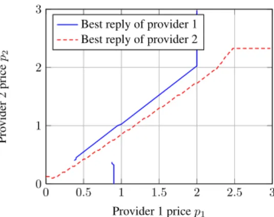
0 0.5 1 1.5 2 2.5 3 0 1 2 3 Provider 1 price p1 Pro vider 2 price p2
Best reply of provider 1 Best reply of provider 2
Figure 1. Curves of best-reply prices for Example4.1.
Each provider i∈ N tries to maximize her revenue Ri(p) ∶= pi ∑
t∈Si di,t(p),
defined as the product of the price charged and the total demand at provider i.
The equilibrium notion in this case is the so-called Nash equilibrium, which is a price profile p∗ such that no provider, acting selfishly, can increase her revenue by an unilateral deviation. Formally, a Nash equilibrium is a price profile p∗such that∀i ∈ N ,
∀pi≥0 Ri(p∗i;p∗−i) ≥ Ri(pi;p∗−i)
where(pi;p∗−i) is vector p∗with price p∗i of operator i replaced by pi.
A Nash equilibrium does not necessarily exist, as illustrated by the following example.
Example 4.1. Consider a scenario with two providers proposing both an owned-spectrum technology,
and such that demand and congestion cost functions are defined by
D(x) = [4 − x]+ ℓ1(d1) = 1 (5 − d1)5− 1 55 ℓ2(d2) = 1 (3 − d2)5− 1 35
Then there is no Nash equilibrium for the pricing game. To illustrate this, Figure 1 displays the best response curves of providers (i.e., prices maximizing their revenue) in terms of the price of the competitor. A Nash equilibrium should be an intersection point of those two curves. Here, there is no intersection point, due to a discontinuity in Player 2’s best response at aroundp2=0.39. This comes
from the fact that the revenue curve of Player 2 has two local maxima for a givenp1, and the global
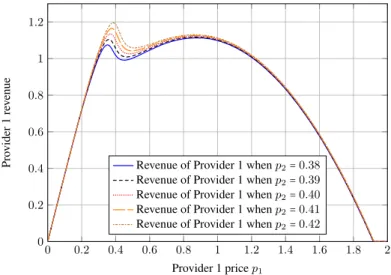
maximum switches from one to the other. This transition is illustrated in Figure2.
Though, in all practical scenarios that will be investigated in Section6, when both operators propose owned spectrum technologies, a unique Nash equilibrium exists and is non null.
0 0.2 0.4 0.6 0.8 1 1.2 1.4 1.6 1.8 2 0 0.2 0.4 0.6 0.8 1 1.2 Provider 1 price p1 Pro vider 1 re v enue
Revenue of Provider 1 when p2=0.38
Revenue of Provider 1 when p2=0.39
Revenue of Provider 1 when p2=0.40
Revenue of Provider 1 when p2=0.41
Revenue of Provider 1 when p2=0.42
Figure 2. Provider 1 revenue as a function of prices of both providers.
Proposition 4.1. Under Assumption 3.1, at a Nash equilibrium with strictly positive prices, each technology inTs(i.e., shared-spectrum) is used by at most a single operator.
Proof: To establish the proposition, we apply a result from [17], where a model similar to ours is used, but no shared technologies are involved. In that paper, Hayrapetyan, Tardos, and Wexler establish that the Wardrop equilibrium repartition is continuous in the price profile. In our case, each shared technology t ∈Tpcan be seen as a single option (i.e., regardless of the provider chosen) with a charge
price pt∶= min{pj, t ∈ Sj}, and a congestion cost ℓt(∑jdj,t). Since min{pj, t ∈Sj} is continuous
in the price profile, then so is the total flow on each shared technologies, as well as flows on each owned-spectrum technology t ∈Ts.
Suppose that there exists a Nash equilibrium with a shared-spectrum technology t ∈Tsfor which at
least two providers have a positive demand.
Remark first that in that case, the providers have declared the same price p. Indeed, from (3) the perceived price at those providers are necessarily the same due to the fact that they have a positive demand, and the congestion cost is the same for both providers on that shared technology.
Let us consider a provider i that does not obtain all the demand on technology t at the Wardrop equilibrium, i.e., d∗i,t<∑j∶t∈Sjd
∗
j,t∶= d∗t. Then consider that operator decreasing her price by a small
amount ε > 0. Consequently, by a small decrease of one’s price, provider i would only slightly affect demand on her owned-spectrum technologies, but will be the only cheapest provider on technology t, and thus get all demand (itself being slightly modified) on that technology. Likewise, if provider i operates on other shared technologies, her demand does not decrease on those. Therefore, when ε tends to 0, the change in revenue for provider i tends to a value that is at least pi(d∗t− d∗i,t), which is strictly
positive. Provider i can then choose ε small enough to strictly improve her revenue, which contradicts
the price profile being a Nash equilibrium. ∎
A Nash equilibrium of the pricing game does not always exist. However, when there is one, the prices set by providers satisfy a relation similar to the ones proved in [12,13].
concave and differentiable with bounded differential functionD′. Further assume that all congestion functionsℓtand ℓi,t are such that ℓt(0) = ℓi,t = 0, i.e., no congestion means no cost. Then at any
Nash equilibrium(p∗1, . . . , p∗N) of the pricing game, with corresponding demands (d∗i,t)1≤i≤N,t∈Si and
perceived price ¯p, we have p∗i = d∗i ∑k∈Si 1 ℓ′ i,k(d ∗ i,k) + d∗i (∑j≠i∑t∈Sj 1 ℓ′ j,t(d ∗ j,t)) − D ′(¯p) , (4) where d∗i ∶= ∑t∈Sid ∗
i,t is the total demand of provideri and d∗ ∶= ∑i∈Nd∗i is the overall demand.
Remark that the right-hand side of (4) can be completely expressed in terms of demands, since ¯p is the
solution ofD(¯p) = d.
The proof is provided in the Appendix.
5. THIRD LEVEL OF GAME: COMPETITION ON TECHNOLOGIES
At an even larger time scale, providers have to decide which technologies to operate. Here again, their decisions will depend on the anticipation about what their revenue would be at the equilibrium of the intermediate level, for any profileS = (S1, . . . ,SN) of strategies implemented by the operators. The
goal is therefore for each provider i to determine the combination of technologiesSi ⊂T which will
maximize her revenue, taking into account the implementation (infrastructure plus licence) costs. Formally, each provider can choose her (finite) subset of technologies, resulting in a (multidimensional) matrix of revenues (R1(S), . . . , RN(S))S∈TN. Similarly, let ci,t represent the licence and infrastructure costs to provider i to operate on technology t. For simplicity of the presentation, those costs are assumed additive, such that the cost of implementingSifor i is∑t∈Sici,t,
but one can without any added complexity consider a general cost function ci(Si). Those costs ci,tcan
be highly asymmetric because some providers may already own an infrastructure, or a part of it, and/or a licence, when it is required. The goal of each provider i is at this time scale also to maximize her net benefit Bi(S) = Ri(S) − ∑ t∈Si ci,t= ∑ t∈Si (p∗ id∗i,t− ci,t),
given that competitors proceed similarly. The equilibrium notion is here again that of a Nash equilibrium, which is a profile S∗ of implemented technologies, such that no provider can improve her benefit by changing unilaterally her set of technologies:
∀i ∈ {1, . . . , N}, ∀Si⊂T , Bi(S∗) ≤ Bi(Si;S−i∗)
where(Si;S−i∗) is vector S∗withSi∗replaced bySi. Note that the set of strategies is finite here instead
of continuous in the previous section.
In the next section, we consider specific situations and analyze the existence and uniqueness of an equilibrium, which cannot be guaranteed in general. We will consider the situation of N = 2 providers in competition. We will therefore end up with two matrices:
• a matrix of revenues from subscribers
R∶= (R1(S), R2(S))S
1,S2⊂T
giving for each combination of technology choices, the respective revenues of the two providers at the equilibrium of the pricing game, obtained from Section4;
• and a cost matrix
C =(c1(S), c2(S))S
1,S2⊂T . From those two matrices, the net benefit matrix
R− C = (R1(S) − c1(S), R2(S) − c2(S))S
1,S2⊂T
is deduced. A Nash equilibrium, if any, is then an element of that last matrix such that the first coordinate R1− c1 is maximal over the lines, and the second coordinate R2− c2 is maximal over
the columns.
If in general, we may have several and non-symmetric Nash equilibria, one of them may be more relevant, be it from users point of view, or regarding the overall wealth generated by the resources (here, the radio spectrum). We therefore introduce corresponding measures, that can be computed for each technology profile.
Define the valuation function V as the total money that customers are ready to spend in order to buy q flow units, i.e.,
V(q) = ∫
q
0 v(q)dq, (5)
where v is the generalized inverse of the demand function D, i.e., v(q) = min{p ∶ D(p) ≤ q}. Define also the user welfare as the difference between the money customers are ready to spend, and the total price they actually pay to buy q flow units,
U W = V(q) − v(q) × q.
As a last definition, we call social welfare, noted SW , the sum of utilities of all actors in the game: • customers, with aggregate utility represented by the user welfare,
• providers, with utility Rj− cjfor provider j,
• and licence sellers and infrastructure sellers, with respective total revenues Rlsand Ris
Hence, SW = U W+ Rls+ Ris+ N ∑ j=1(R j− cj) = U W+ N ∑ j=1 Rj,
the last equality coming from Rls+Ris=∑Nj=1cjbecause revenues of licence and infrastructure sellers
are exactly the sum of costs of providers. From the customers point of view (resp. from the point of view of the society as a whole: users, providers, licence seller, infrastructure sellers) the most interesting Nash equilibrium is the one maximizing user welfare (resp. social welfare).
6. PRACTICAL EXAMPLES
We now apply our model to some particular contexts of telecommunication operator competition. In the case of the competition among french wireless providers in 2010, we present a technology choice analysis with a WiMAX deployment option for two operators.
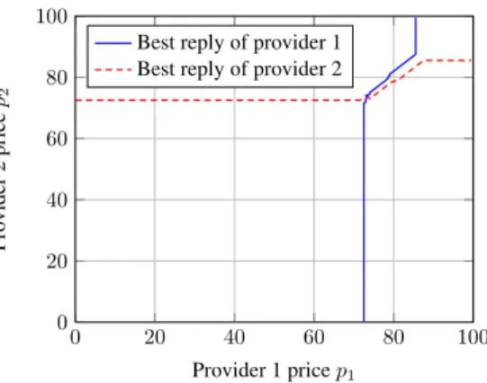
0 20 40 60 80 100 0 20 40 60 80 100 Provider 1 price p1 Pro vider 2 price p2
Best reply of provider 1 Best reply of provider 2
Figure 3. Curves of best-reply prices when both players propose the WiMAX technology.
6.1. Intermediate level pricing game
We first focus on the game on prices at the intermediate level, ignoring for the moment the licence and infrastructure costs. Formally, we build the revenue matrix R defined in the previous section.
We assume that a set of users is positioned in a bounded predefined zone, and that all users have a terminal with multiple interfaces. We have in mind a specific zone covered by a 3G UMTS base station in France. There are approximately 104such zones on the French territory. We additionally assume that the zone is covered by a WiFi 802.11g access point and a single 802.16e (WiMAX) base station. We only consider downlink for convenience and choose realistic values of demand and capacities:
• 28 Mb/s per operator for 3G [18];
• 40 Mb/s, still in downlink, for WiMAX technology [19]; • 25 Mb/s for WiFi [20].
We moreover assume the demand function D to be linear on its support, given by (in Mb/s) D(¯p) = [300 − 3¯p]+,
with ¯p in e/month. Hence no user is willing to pay more than 100 e monthly to benefit from the service. In our numerical computations, the congestion function ℓi,t of a couple demand-technology
(i, t) is supposed to be the average waiting time of a M/M/1 queue of parameters (di,t, Ci,t) if the
technology t belongs to the setTp, and of parameters(∑t∈Sidi,t, Ct) if t belongs to Ts. Recall that the average waiting time of an M/M/1 queue with parameters(λ, µ) is 1/(µ − λ) − 1/µ.
To illustrate how those Nash equilibria are found, consider for instance the case where the two operators decide to propose only a WiMAX access to the users. Figure3displays the best responses (i.e., prices maximizing their revenue) of providers in terms of the price of the other. A Nash equilibrium is an intersection point of those two curves. One can check that there exists a single non-null intersection point between the two curves, here approximately equal to(72.5, 72.5). For the practical examples studied in this paper, we proceeded numerically to compute best-replies of both providers, and find the Nash equilibria on prices (actually, we always found either one unique Nash equilibrium, or no equilibrium at all).
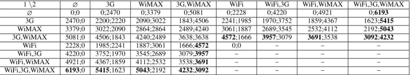
TableIdisplays the monthly revenues in euros of both operators at the Nash price profile, for every technology profile. On each element of the table, the first number is the revenue of Provider 1, while the
1\2 ∅ 3G WiMAX 3G,WiMAX WiFi WiFi,3G WiFi,WiMAX WiFi,3G,WiMAX ∅ 0;0 0;2470 0;3379 0;5081 0;2228 0;4220 0;4921 0;6193 3G 2470;0 2200;2220 2090;3022 1843;4506 2241;1985 1970;3752 1859;4367 1623;5415 WiMAX 3379;0 3022;2090 2864;2864 2489;4240 3061;1887 2689;3545 2532;4112 2192;5043 3G,WiMAX 5081;0 4506;1843 4240;2489 3638;3638 4572;1666 3957;3079 3691;3538 3092;4232 WiFi 2228;0 1985;2241 1887;3061 1666;4572 0;0 − − − WiFi,3G 4220;0 3752;1970 3545;2689 3079;3957 − − − − WiFi,WiMAX 4921;0 4367;1859 4112;2532 3538;3691 − − − − WiFi,3G,WiMAX 6193;0 5415;1623 5043;2192 4232;3092 − − − −
Table I. Revenues matrix (from users) for providers depending on the implemented technologies.
1\2 ∅ 3G WiMAX 3G,WiMAX WiFi WiFi,3G WiFi,WiMAX WiFi,3G,WiMAX
∅ 0.0 74 182 662 54 384 600 1396 3G 74 486 726 1442 408 938 1262 2282 WiMAX 182 726 975 1785 662 1368 1755 2709 3G.WiMAX 662 1442 1785 2799 1368 2305 2799 4087 WiFi 54 408 662 1368 103 - - -WiFi.3G 384 938 1368 2305 - - - -WiFi.WiMAX 600 1262 1755 2799 - - - -WiFi.3G.WiMAX 1395 2282 2709 4087 - - -
-Table II. User welfare depending on the implemented technologies.
second is the revenue of Provider 2. We can notice a direct consequence of Proposition4.1: when both operators choose to implement the WiFi technology, then if a Nash exists (which is when they operate WiFi only), then they both end up with a null revenue. The price equilibrium is when both providers set their price to 0: from that situation, no provider can unilaterally change her price and get a strictly positive revenue, since setting a strictly positive price implies that all users on the shared technology -here thus, all the demand- go to the competitor. In all other cases where the operators implement WiFi but at least one provider operates another technology, no Nash equilibrium actually exists, because at the only possibility(0, 0), any provider operating an unshared technology could increase her price and make profit on that technology. We thus end up with the “−” symbol in TableIto represent that no Nash equilibrium exists.
Best responses of providers, in terms of technology sets, are displayed in bold in the Table. A Nash equilibrium is therefore easily spotted as cells with both numbers on bold. If we considered the game on technologies without any implementation cost, we would then have two possible (and symmetric) Nash equilibria, ({WiFi, 3G, WiMAX}, {3G, WiMAX}) and ({3G, WiMAX}, {WiFi, 3G, WiMAX}). We now aim at investigating for different scenarios the outcome of the game on technologies, as well as the selection of those equilibria from a user and social welfare optimization point of view.
6.2. Symmetric game
Consider again, as well as in the rest of the paper, a zone covered by a single base station, for a period of one month. Estimated infrastructure plus licence costs, if any, are therefore also divided by the 104 zones in France and by the duration in months of the licence rights. As presented in Section5, we define a cost per zone and per month at provider i for technology t and a cost matrix(c1(S1), c2(S2))S
1\2 ∅ 3G WiMAX 3G,WiMAX WiFi WiFi,3G WiFi,WiMAX WiFi,3G,WiMAX ∅ 0 2544 3561 5742 2282 4604 5521 7588 3G 2544 4886 5838 7791 4634 6660 7488 9320 WiMAX 3561 5838 6703 8514 5610 7602 8399 9944 3G.WiMAX 5743 7791 8514 10075 7606 9341 10028 11411 WiFi 2282 4634 5610 7606 103 - - -WiFi.3G 4604 6660 7602 9341 - - - -WiFi.WiMAX 5521 7488 8399 10028 - - - -WiFi.3G.WiMAX 7588 9320 9944 11411 - - -
-Table III. Social welfare depending on the implemented technologies.
1\2 ∅ 3G WiMAX 3G,WiMAX WiFi WiFi,3G WiFi,WiMAX WiFi,3G,WiMAX
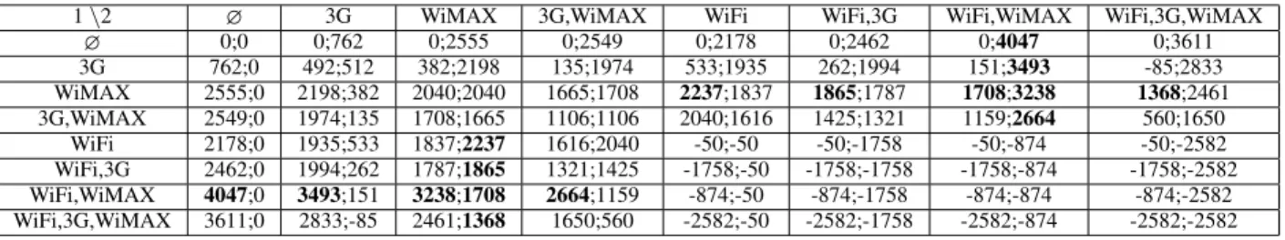
∅ 0;0 0;762 0;2555 0;2549 0;2178 0;2462 0;4047 0;3611 3G 762;0 492;512 382;2198 135;1974 533;1935 262;1994 151;3493 -85;2833 WiMAX 2555;0 2198;382 2040;2040 1665;1708 2237;1837 1865;1787 1708;3238 1368;2461 3G,WiMAX 2549;0 1974;135 1708;1665 1106;1106 2040;1616 1425;1321 1159;2664 560;1650 WiFi 2178;0 1935;533 1837;2237 1616;2040 -50;-50 -50;-1758 -50;-874 -50;-2582 WiFi,3G 2462;0 1994;262 1787;1865 1321;1425 -1758;-50 -1758;-1758 -1758;-874 -1758;-2582 WiFi,WiMAX 4047;0 3493;151 3238;1708 2664;1159 -874;-50 -874;-1758 -874;-874 -874;-2582 WiFi,3G,WiMAX 3611;0 2833;-85 2461;1368 1650;560 -2582;-50 -2582;-1758 -2582;-874 -2582;-2582
Table IV. Benefits matrix for the symmetric game.
In this symmetric game, we consider two incoming providers without any wireless infrastructure paying the same infrastructure and licence costs. A total 3G licence of 649 Me [21] needs to be paid to the regulation authority, and 3G infrastructure of 1.4Be (value inspired from [22]) has to be purchased, both monthly paid over 10 years. Hence, the licence cost (resp. the infrastructure cost) is then evaluated to 541 e (resp. 1167 e) per month and per zone, giving c1,3G=c2,3G=1708 e. We also assume that a
licence costs 649 Me for WiMAX and the infrastructure costs 340 Me (inspired from [23]), yielding c1,WiMAX =c2,WiMAX=541+ 283 = 824 e. We assume that every WiFi access point is renewed each
year and is bought at the average price of 600 e per year. In France, since only a declaration to the regulation authority, negligible taxes an no licence purchase are necessary to deploy and use a WiFi infrastructure [24,25], we then choose c1,WiFi=c2,WiFi=50 e.
The resulting benefits matrix (revenue matrix minus cost matrix) is displayed in Table IV. It can be readily checked that there exists two Nash equilibria, ({WiFi,WiMAX},{WiMAX}) and ({WiMAX},{WiFi,WiMAX}).
In that case, we remark in TableIVthat there are two Nash equilibria, ({WiFi,WiMAX},{WiMAX}) and ({WiMAX},{WiFi,WiMAX}). With respect to the previous situation, 3G is actually too expensive with the proposed licence cost to be implemented . Since those Nash equilibria on technologies are symmetric, user and social welfare values are the same and no preference can be defined.
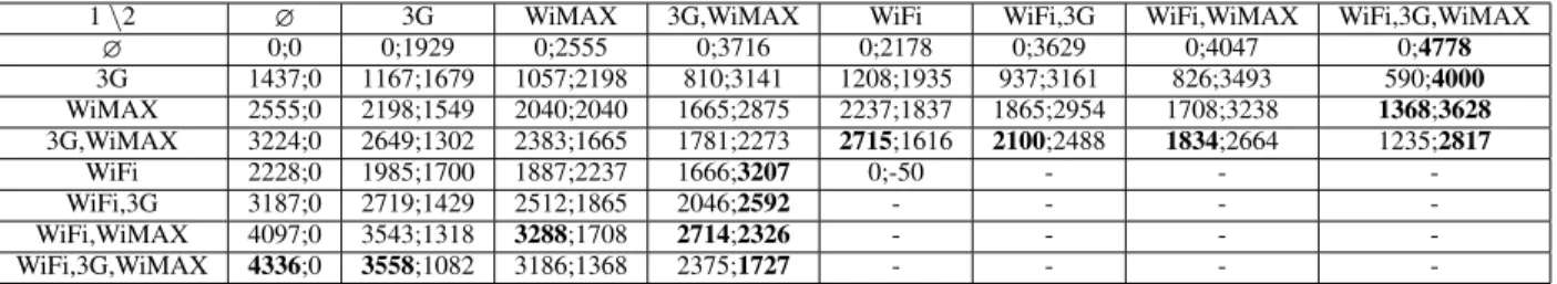
6.3. A WiFi-positionned provider against a 3G one
Consider a WiFi-installed provider, named Provider 1, wishing to extend her position against a 3G-installed provider, noted Provider 2. We suppose that Provider 1 already owns a complete WiFi infrastructure over the 104zones (basically like the provider called Free in France) and that Provider 2
1\2 ∅ 3G WiMAX 3G,WiMAX WiFi WiFi,3G WiFi,WiMAX WiFi,3G,WiMAX ∅ 0;0 0;1929 0;2555 0;3716 0;2178 0;3629 0;4047 0;4778 3G 1437;0 1167;1679 1057;2198 810;3141 1208;1935 937;3161 826;3493 590;4000 WiMAX 2555;0 2198;1549 2040;2040 1665;2875 2237;1837 1865;2954 1708;3238 1368;3628 3G,WiMAX 3224;0 2649;1302 2383;1665 1781;2273 2715;1616 2100;2488 1834;2664 1235;2817 WiFi 2228;0 1985;1700 1887;2237 1666;3207 0;-50 - - -WiFi,3G 3187;0 2719;1429 2512;1865 2046;2592 - - - -WiFi,WiMAX 4097;0 3543;1318 3288;1708 2714;2326 - - - -WiFi,3G,WiMAX 4336;0 3558;1082 3186;1368 2375;1727 - - -
-Table V. Benefits matrix for the WiFi-3G game.
similarily owns a complete 3G infrastructure over the same zones (Bouygues Telecom for instance). Bouygues Telecom already owning an infrastructure, only its licence cost of 649 Me accounts, giving c2,3G=541 e. The cost of the fourth licence in France (the one Free is buying) is fixed to 240 Me [21],
and of the new infrastructure estimated at 1.0 Be (value inspired from [22]), so that c1,3G=1033 eper
month and per site. For WiFi, we choose c1,WiFi=0 eand c2,WiFi=50 eto illustrate the better position
of Provider 1, while WiMAX costs are the same as in the previous subsection (that technology being a new one). The benefits matrix is given in TableV, with again best responses highlighted in bold. For this game, there are two non symetric Nash equilibria. The first one is ({WiFi,WiMAX},{3G,WiMAX}): each operator chooses the technology on which she is already present, and additionally goes to the new WiMAX technology. The second Nash equilibrium is ({WiMAX},{WiFi,3G,WiMAX}) and corresponds to a situation where Provider 2 proposes all technologies and Provider 1 only proposes the WiMAX technology. Again, it is better not to fight on (the low-cost) WiFi.
Since the ({WiFi,WiMAX},{3G,WiMAX}) results in a computed social welfare SW = 10028, and the ({WiMAX},{WiFi,3G,WiMAX}) equilibrium yields SW = 9944, the first one would be better-suited in terms of social welfare. Similarily, user welfare values are respectively 2799 and 2709, the first equilibrium is more advised from the users point of view too.
It is possible to vary the Nash equilibria set by changing licences prices. Indeed, obtaining a Nash equilibrium with 3G implemented by Provider 1 requires the cost c1,3G to be reduced to 900 e (the
situation ({WiMAX},{WiMAX,WiFi,3G})) is not an equilibrium anymore if this cost is reduced even more). This would mean a licence fee of 67 e (or equivalently a global 3G licence selling price of 80 Me). In that case, the situation ({3G,WiMAX},{WiFi,3G,WiMAX}) would be a third Nash equilibrium of the technological game: Provider 1 would focus on licenced technologies, giving up on WiFi. Social welfare and user welfare values are in this case respectively equal to 11411 and 4087. Those values are the maximal ones that can be attained, as could be expected: it is indeed in the interest of the community to use the maximum of resources (i.e., all the radio spectrum), and this also benefits to users since more available resources correspond to a harder competition for customers and less congestion.
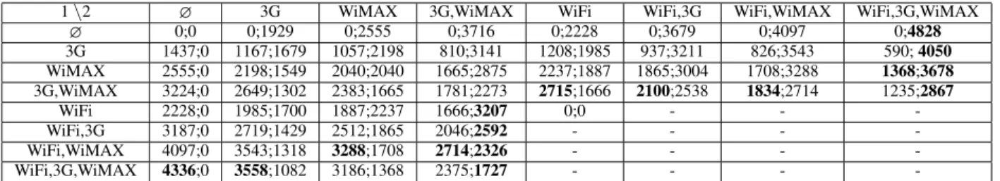
6.4. A single technology-positionned provider against a dominant one
This kind of game would for instance correspond in France to Free (strongly established in the Internet and WiFi networks), named Provider 1 again, against Orange, named Provider 2, already positionned on almost all technologies, except WiMAX, for which we keep the costs of previous subsections. The 3G costs are also considered the same as in the previous subsection, but WiFi costs are here
1\2 ∅ 3G WiMAX 3G,WiMAX WiFi WiFi,3G WiFi,WiMAX WiFi,3G,WiMAX ∅ 0;0 0;1929 0;2555 0;3716 0;2228 0;3679 0;4097 0;4828 3G 1437;0 1167;1679 1057;2198 810;3141 1208;1985 937;3211 826;3543 590; 4050 WiMAX 2555;0 2198;1549 2040;2040 1665;2875 2237;1887 1865;3004 1708;3288 1368;3678 3G,WiMAX 3224;0 2649;1302 2383;1665 1781;2273 2715;1666 2100;2538 1834;2714 1235;2867 WiFi 2228;0 1985;1700 1887;2237 1666;3207 0;0 - - -WiFi,3G 3187;0 2719;1429 2512;1865 2046;2592 - - - -WiFi,WiMAX 4097;0 3543;1318 3288;1708 2714;2326 - - - -WiFi,3G,WiMAX 4336;0 3558;1082 3186;1368 2375;1727 - - -
-Table VI. Benefits matrix for the WiFi-Dominant game.
c1,WiFi = c2,WiFi = 0 edue to the past presence of both providers on this technology. The results of
the technological game are displayed in TableVI. One can see here that, again, two Nash equilibria exist and are the same as those of the previous game in part6.3, with user and social welfare equal to 2799 and 10028 for the first equilibrium, and 2709 and 9944 for the second one. That is, the existence of the WiFi infrastructure for Provider 2 does not affect the Nash equilibria. Hence, we deduce that the impact of the WiFi infrastructure cost is negligible compared to the 3G and WiMAX licence and infrastructure costs. Similarly, if the monthly cost per site for 3G gets as low as 694 e, then Provider 1 could keep operating WiFi, since the situation ({WiFi,3G,WiMAX},{3G,WiMAX}) would arise as a technological Nash equilibrium. In that case, the monthly licence cost would be equal to 153 e (the total licence price would be equal to 184Me). The social welfare and user welfare values are in this case respectively 11411 and 4087. Hence reducing the 3G costs would be beneficial, since this last Nash equilibrium yields larger user and social welfare values.
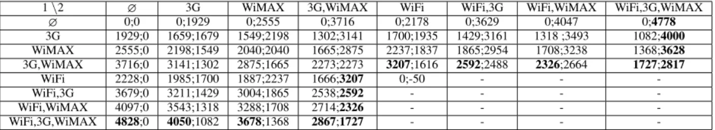
6.5. A 3G technology-positioned provider against an omnipresent one
This last scenario corresponds in France to Bouygues Telecom (Provider 1, operator only owning a 3G infrastructure), against SFR (Provider 2, owning a 3G and WiFi infrastructure). The WiMAX infrastructure and licence costs are again assumed to be the same as before for both operators. In addition, the WiFi infrastructure cost is assumed to be equal to 50 eper month. The 3G licence cost is also equal to 541 e, given that both licences are supposed equal to 649 Meand paid over 10 years. We can notice on Table VIIthat there exist two symmetric Nash equilibria on technologies which are ({WiFi, 3G, WiMAX},{3G,WiMAX}) and ({3G, WiMAX},{WiFi, 3G,WiMAX}). Both providers have an interest to invest in the WiMAX technology and to keep their 3G infrastructure active. This conclusion contrasts with the one opposing a 3G operator to a dominant one depicted in Table VI. Since the found Nash equilibria maximize the user and social welfare values among every technology combinations of operators, no new interesting Nash equilibrium on technologies would come from a 3G licence price variation.
7. CONCLUSION
In this paper, we have presented a three-level competition model on technology investments among wireless telecommunications service providers. Each level corresponds to a different time scale. At a first level, users choose the couple operator-technology offering them the best compromise between congestion and price per flow unit, where total demand is supposed elastic. Some demand can be
1\2 ∅ 3G WiMAX 3G,WiMAX WiFi WiFi,3G WiFi,WiMAX WiFi,3G,WiMAX ∅ 0;0 0;1929 0;2555 0;3716 0;2178 0;3629 0;4047 0;4778 3G 1929;0 1659;1679 1549;2198 1302;3141 1700;1935 1429;3161 1318 ;3493 1082;4000 WiMAX 2555;0 2198;1549 2040;2040 1665;2875 2237;1837 1865;2954 1708;3238 1368;3628 3G,WiMAX 3716;0 3141;1302 2875;1665 2273;2273 3207;1616 2592;2488 2326;2664 1727;2817 WiFi 2228;0 1985;1700 1887;2237 1666;3207 0;-50 - - -WiFi,3G 3679;0 3211;1429 3004;1865 2538;2592 - - - -WiFi,WiMAX 4097;0 3543;1318 3288;1708 2714;2326 - - - -WiFi,3G,WiMAX 4828;0 4050;1082 3678;1368 2867;1727 - - -
-Table VII. Benefits matrix for the 3G-Dominant game.
possibly be shared among providers under a predefined rule based on their reputation. At a second level, operators choose their price per flow unit maximizing their revenue at the obtained flow distribution, such that no one would have an incentive to change it. At a third level, operators choose the technology combination maximizing their revenue, which is based on the price and flow distribution of the previous levels and the infrastructure and licence costs. We illustrate our model with a simple competition study among french wireless operators, where considered technologies are 3G, WiMAX and WiFi. Hence, given some initial infrastructure or licence price reduction, it has been shown in the four scenarios opposing two operators that it is in their interest to invest in the WiMAX infrastructure. A licence cost reduction can be necessary in some cases, because this reduction can generate a new equilibrium on technologies maximizing the social welfare.
The work presented in the paper can be extended in several ways. A first possibility is to adapt the model to an unshared technology zone covered by several shared technology subzones under similar flow equilibrium constraints. A second way to model this is to modify the model such that some smooth increase of a minimal perceived price does not jeopardize the whole corresponding demand and to analyze the existence of price equilibrium in the case where technologies are shared. Finally, customers may not have multiple interfaces, i.e., they may not be able to choose among all technologies. This heterogeneity could be taken into account.
Acknowlegment
This paper is an extended version of a paper submitted to IEEE Globecom 2010 (reference [1]).
The authors would like to acknowledge the support of the ANR Verso Project CAPTUREShttp:
//captures.inria.fr/
APPENDIX: Proof of Proposition4.2
Proof: First, if a Nash equilibrium exists, then from Proposition 4.1, there are no shared-spectrum technologies for which more than one provider obtain some demand. But at a Nash equilibrium, any shared-spectrum technology t ∈ Ts gets some demand: if this were false, this would mean that all
operators of t have a price above ¯p and thus get no revenue, while they could obtain a strictly positive revenue by choosing a price strictly below ¯p.
with strictly positive demand) by exactly one provider, that is the cheapest one among the operators of that technology. As a result, infinitesimal price variations from providers do not change the identity of the cheapest ones on shared-spectrum technologies. A consequence is that in a vicinity of the Nash price profile(p∗1, . . . , p∗N), each shared-spectrum technology behaves exactly as if is were an
owned-spectrum technology of its cheapest operator.
We can therefore apply Proposition 2 of [13], where all links (in our context, technologies) are owned by providers, but only the property of Nash equilibria being local maxima of revenues is used. That property can also be used in our model, considering all technologies as (locally) owned-spectrum ones. The only difference from [13] is that we allow here providers to operate on several technologies. However, since they declare a unique price and demand distributes itself according to a Wardrop equilibrium, then all technologies for a provider have the exact same perceived cost (this should hold only for technologies with demand, but here all technologies get demand since ℓi,t(0) = 0 for all t ∈ Si),
and therefore the same congestion cost ℓi,t(di,t). If a provider gets a total demand di=∑t∈Sidi,t, we refer to that common value of the congestion cost by ℓi(di), which should satisfy:
∀di≥0, ℓi(di) = ℓi,t(xt) ∀t ∈ Si (6)
s.t. xt≥0, ∑
t∈Si
xt=di. (7)
Now consider an infinitesimal variation of ε from an initial di>0. We denote by εtthe corresponding
variation of xt, for each t ∈Si. From (6), we have for all t ∈Si, ℓi(di+ ε) = ℓi,t(xt+ εt). Since the
functions ℓi,t are strictly increasing and concave, εt =O(ε), and moreover xt >0and ℓ′i,t(xt) > 0.
Thus,
ℓi(di+ ε) = ℓi,t(xt+ εt) = ℓi,t(xt) + εtℓ′i,t(xt) + o(εt)
= ℓi(di) + εtℓ′i,t(xt) + o(ε), and therefore εt=
ℓi(di+ε)−ℓi(di)
ℓ′
i,t(xt) + o(ε). Then (7) yields ∑ t∈Si εt=(ℓi(di+ ε) − ℓi(di)) ∑ t∈Si 1 ℓ′i,t(xt) + o(ε) = ε, which implies that ℓiis differentiable, with derivative
ℓ′i(di) = 1 ∑t∈Si 1 ℓ′ i,t(xt) . (8)
As a result, from the provider point of view, the set of technologiesSibehaves exactly as a unique
technology that would have a congestion cost function ℓi. Moreover, since ℓi,tis convex for all t, so is
ℓi. Proposition4.2is then directly obtained by plugging (8) into the Proposition 2 of [13]. ∎
REFERENCES
1. P. Maill´e, B. Tuffin, and J.-M. Vigne. Economics of technological games among telecommunication service providers. Submitted, available at http://www.rennes.enst-bretagne.fr/˜pmaille/papiers/tech_submit. pdf, 2010.
2. IEEE 802.16-2004. IEEE Standard for Local and Metropolitan Area Networks - Part 16: Air Interface for Fixed Broadband
3. J.G. Wardrop. Some theoretical aspects of road traffic research. Proc. of the Institute of Civil Engineers, 1:325–378, 1952. 4. M.J. Osborne and A. Rubenstein. A Course on Game Theory. MIT Press, 1994.
5. D. Acemoglu and A. Ozdaglar. Competition and efficiency in congested markets. Mathematics of Operations Research, 2006.
6. F. Bernstein and A. Federgruen. A general equilibrium model for industries with price and service competition.
Management Science, 52(6):868–886, 2004.
7. P. Maill´e and B. Tuffin. Analysis of price competition in a slotted resource allocation game. In Proc. of IEEE INFOCOM
2008, Phoenix, AZ, USA, April 2008.
8. P. Maill´e and B. Tuffin. Price war with partial spectrum sharing for competitive wireless service providers. In Proceedings
of IEEE Globecom, December 2009.
9. M.H. Manshaei, J. Freudiger, M. Felegyhazi, P. Marbach, and J.P. Hubaux. On wireless social community networks. In
Proc. of IEEE INFOCOM, Phoenix, AZ, USA, Apr 2008.
10. Y. Xing, R. Chandramouli, and C. Cordeiro. Price dynamics in competitive agile spectrum access markets. Selected Areas
in Communications, IEEE Journal on, 25(3):613–621, April 2007.
11. P. Njoroge, A. Ozdaglar, N. Stier-Moses, and G. Weintraub. Competition, market coverage, and quality choice in interconnected platforms. In Proceedings of the Workshop on the Economics of Networked Systems (NetEcon), 2009. 12. R. Johari, G. Y. Weintraub, and B. Van Roy. Investment and market structure in industries with congestion. Operations
Research, submitted.
13. A. Ozdaglar. Price competition with elastic traffic. Networks, 52(3):141–155, 2008.
14. M. Beckmann, C. B. McGuire, and C. B. Winsten. Studies in the economics of transportation. Yale University Press, New Heaven, Connecticut, 1956.
15. H.Z. Aashtiani and T.L. Magnanti. Equilibria on a congested transportation network. SIAM Journal of Algebraic and
Discrete Methods, 2:213–226, 1981.
16. T. Roughgarden. Selfish Routing and the Price of Anarchy. MIT Press, 2005.
17. A. Hayrapetyan, ´E. Tardos, and T. Wexler. A network pricing game for selfish traffic. In Proc. of ACM SIGACT-SIGOPS
Symposium on Principles of Distributed Computing (PODC), 2005.
18. 01NetPro. Le d´ebit sur le r´eseau 3G d’Orange passe `a 14 mb/s, January 2010. http://pro.01net.com/
editorial/511553/le-debit-sur-le-reseau-3g-dorange-passe-a-14-mbits-s/.
19. Wireless design mag. WiMAX 101 : the Evolution of WiMAX, 2010. http://www.wirelessdesignmag.com. 20. Wikip´edia. WiFi. http://fr.wikipedia.org/wiki/Wi-Fi.
21. Mobinaute. 4`eme licence 3G : Orange fait pression aupr`es du gouverne-ment pour ralentir son attribution, October 2009. http://www.mobinaute.com/ 304016-4eme-licence-3g-orange-pression-aupres-gouvernement-ralentir-attribution.
html.
22. Capital. Mobiles : comment Free compte faire baisser les prix, May 2009. http://www.capital.fr/enquetes/
strategie/mobiles-comment-free-compte-faire-baisser-les-prix-380294.
23. Wimaxday. Worldmax launches mobile WiMAX network, June 2008.http://www.wimaxday.net/site/2008/
06/17/worldmax-launches-mobile-wimax-network.
24. 01NetPro. Le Wi-Fi devient officiellement une activit´e commerciale, May 2007. http://pro.01net.com/
editorial/348616/le-wi-fi-devient-officiellement-une-activite-commerciale/.
25. Arcep. D´ecision no. 2007-0408 de l’autorit´e de r´egulation des communications ´electroniques et des postes en date du 26 avril 2007 mettant fin au r´egime d’exp´erimentation de r´eseaux ouverts au public utilisant la technologie rlan, April 2007.