Development of a radar simulator for monitoring wake vortices in rainy weather

To cite this document:

Liu, Zongxhun and Jeannin, Nicolas and Vincent, François

and Wang, Xuesong Development of a radar simulator for monitoring wake

vortices in rainy weather. (2011) In: Radar 2011 International Conference of

radar (CIE), 24-27 October, 2011, Chengdu, China.

O

pen

A

rchive

T

oulouse

A

rchive

O

uverte (

OATAO

)

OATAO is an open access repository that collects the work of Toulouse researchers and

makes it freely available over the web where possible.

This is an author-deposited version published in:

http://oatao.univ-toulouse.fr/

Eprints ID: 5238

Any correspondence concerning this service should be sent to the repository

administrator:

staff-oatao@inp-toulouse.fr

Development of a Radar Simulator for Monitoring

Wake Vortices in Rainy Weather

Z. Liu

, N. Jeannin

, F. Vincent

, X. Wang

1

University of Toulouse, ISAE, 10 Avenue Edouard Belin, 31400, Toulouse, France

2

Colleage of Electronic Science and Engineering, National University of Defense Technology, Changsha, 410073, P.R.China

Email: zhongxun.liu@gmail.com

3

Department of Electromagntic and Radar, ONERA, 2 Avenue Edouard Belin, 31400, Toulouse, France Email: nicolas.jeannin@onera.fr

Abstract

A simulator for the evaluation of the radar signature of raindrops within wake vortices is presented. Simulated Doppler spectrum of raindrops within vortices let to think that it could be a potential criterion for identifying wake vortex hazard in rainy weather.

Keywords: Radar Simulator, Wake vortex, Raindrops, Doppler spectrum.

1. Introduction

When flying in the atmosphere, an aircraft generates wake vortices which are dangerous for other flying aircrafts. During the taking off and landing phases, the safe separation between two aircrafts is driven by the worst case persistence time of wake vortex. How to monitor wake vortices in real time is one of the key technological difficulties for the improvement of aviation safety and airports capacity. The candidate technologies for wake vortex monitoring include Radar, Lidar, and Sodar. Among them, Sodar has a too short detection range, Lidar is not operational in foggy or rainy weathers and always very expensive to purchase and maintain, while Radar can detect and locate wake vortex within a relatively long distance under all weather conditions [1] [2].

Up to now, most of the research on wake vortex radar sensors has been concentrated on field tests [2] [3]. All these findings from radar trials on wake vortex monitoring are very interesting and encouraging. The theoretical studies on radar scattering mechanisms within wake vortices also have been conducted to provide technological guidance for the development of new wake vortex radar sensors since 1990s. In clear air, the radar reflectivity of wake vortex is caused by Bragg scattering and some fruitful results have been achieved in [1] [4]. In rainy weather, the Radar electromagnetic waves are not severely attenuated by raindrops or fog at short range. Contrarily, the droplets rolled up by the wake vortices are strong scatterers enhancing the intensity of the scattered signals. However, few studies on the radar backscattering of wake vortices in rainy weather have been reported, and there is a wide gap between the research of wake vortex and precipitation until now. Thus, the main objective of the presented simulator is to compute the radar signature of raindrops within wake vortices.

There are three key elements in the development of the radar simulator: raindrops, aircraft wake vortices, and radar. When raindrops fall into the wake vortex flow, their

trajectories and velocities are modified. Therefore the concentration of raindrops within wake vortices may be different from the one in still air. As a consequence it may also have an impact on the radar signatures from different range cells. This paper firstly presents a simplified model to compute the trajectory and velocity of raindrops within wake vortices. Then, from simulated drops sizes, position and velocities, the radar signal is computed. Finally, the particular shape of the Doppler spectrum of the raindrops obtained in wake vortex region is shown to provide potential information for identifying wake vortex hazard in aviation traffic control. 2. Interaction between raindrops and wake vortices

Wake vortex is a kind of turbulence generated by the passage of a flying aircraft in the air. In rainy weather, the falling raindrops are transported by the wake turbulence flow as inertial particles under the influence of gravity and drag forces. To model this interaction, some properties of rain drops established without wake turbulence are recalled for the initialization of the simulations. Then a model of velocity within the vortex flow is presented. The methodology to compute the trajectory of the raindrops is presented afterwards.

2.1. Raindrops size distributions and terminal fall velocity A common assumption made in radar-meteorology is to use a modified gamma distribution to describe the raindrops size distributions in still air. The probability density function of drops N D( ) is hence given by

4 0

( ) D,

N D N D e  m (1) where the exponent  depends on the type of rain, N₀ is a constant reflecting the average spatial density of the drops equal to 8 10 m 6 4 at the ground level, D (mm) is the diameter of the raindrop, and  is related to the rain rate R by

0.21 1

4.1R ,mm

  (2)

where R denotes the rain rate in mm/h. Figure 1(a) presents the size distribution under three different rain rates.

In still air, a falling raindrop reaches its terminal fall velocity VT with the equilibrium between the inertial force

and the drag force acting on the particle [5]. A widely used expression between V_T and the diameter D is given by [6]:

0.4 0 1 2 3 ( ) [ ( )]( ) , T V D   exp  D      m/s (3)

where  =9.65m/s,₁  =10.3m/s,₂  =0.6m/s. ₃ 0.4 0

( / ) is a density ratio correction factor adjusting deviation of the terminal fall velocity due to the air density change with altitude. Figure 1(b) presents the terminal fall velocity of raindrops for the altitude levels: 50m, 1000m, and 4000m.

0 2 4 6 8 0 0.1 0.2 0.3 Raindrops diameter: mm N u m ber d ist ri but io n 1 mm/h 10mm/h 100mm/h 0 2 4 6 8 0 2 4 6 8 10 12 Diameters: mm T e rm inal vel o ci ty : m /s 50 m 1000 m 4000 m

(a) Raindrops size distribution (b) Terminal falling velocity Fig. 1. Parametrization of raindrops in still air. The knowledge of raindrop size distribution and terminal velocities is used in the simulation to initialize the simulations considering a homogenous distribution of raindrops above the vortices.

2.2 Wake vortex velocity model

To depict the tangential velocity distribution of the flow within wake vortices the widely-used Rankine model [7] is considered. For each single vortex, the tangential velocity distribution is approximated by:

2 2 c c 0 c / if ( ) 2 1 if r r r r V r r r r  _         (4)

where V r_( ) (m/s) is the tangential velocity at the distance r (m) from the vortex core. rc (m) is the vortex core radius,

2 0(m /s)

 is the initial circulation determined by the aircraft

flying parameters. In case of an elliptical lift distribution, the circulation is expressed as 0 0 0 , 4 Mg b b Ub      (5)

where M (kg) is the weight of the airplane, U (m/s) is the flying speed, g(m/s )2 is the gravitational acceleration, and  (kg/m3) is the air density, b₀ is the separation between two vortices, b (m) is the aircraft's wingspan.

Fig. 2. The velocity field of two counter-rotating vortices [4] In the aircraft vortex wake region as shown in Figure 2, the local velocity of the flow can be expressed as

L R d

( , )x y V V V

u (6)

where V VL, Rare the velocity component induced by the left

and right vortex separately, Vd is the downwash velocity

caused by the mutual interference between two vortices. 2.3. Motion of raindrops within wake vortices

The interaction between raindrops and wake vortex can be considered as the problem of particles moving in the air flow. Some basic assumptions are made for further analysis: the raindrops are spherical and not deformable, the interaction between raindrops such as collision or coalescence is negligible, the presence of raindrop particles doesn't change the structure of the vortex flow.

Therefore, the motion of a raindrop within wake vortex is governed by the weight and the fluid drag force on it as:

p ( ) drag( ) p

mat F t mg (7)

where t is the time, a is the acceleration of the raindrop,

drag

F is the drag force which depends on the relative position

of raindrops within the vortex flow, m is the mass of the _p

raindrop, g is the downward gravitational acceleration which is taken as negative. For an individual particle moving with velocity vp in the fluid velocity fields u z( p, )t . For raindrops

of spherical shape whose usual diameters D are ranging from 0.5mm to 4mm, the Reynolds number of the flow is sufficiently high ([8]) to consider that the drag force Fdrag is

given by:

 

 









where zp (x yp, p) denotes the raindrop's position,  v is the

relative velocity between the vortex flow and the raindrop and

D

C is the drag coefficient.. For a raindrop with diameter D and density , the drag coefficient _w CD can be derived by the

equilibrium of its weight and the drag force in still air as:

2 2 3 D T D 2 T 4 1 1 1 · 0, 2 4 6 3 w a w a gD C V D D g C V          (9) D

C is assumed to be constant in the following as the impact

of air density variations in the vortex flow on CDis not taken

into consideration. Then, the motion equation of raindrops can be further derived as:

p D 2 T d ( ) | | | | d a t mg m m C A m t       V   v g v v g v v (10)

where A is the cross section of the raindrop with the

assumption of spherical shape. The instantaneous position and velocity of raindrops can be obtained from the above equation.

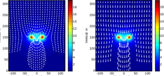
Horizontal: m Ver ti c a l: m -100 -50 0 50 100 0 50 100 150 200 250 300 2 4 6 8 10 12 14 16 18 Horizontal: m Ver ti c a l: m -100 -50 0 50 100 0 50 100 150 200 250 300 2 4 6 8 10 12 14 16 18

(a) D=1.0mm, Duration: 62.2s (b) D=4.0mm, Duration: 31.8s Fig.3. Trajectory and velocity of raindrops in wake vortices

A 4th order four variables Runge-Kutta algorithm has been implemented to solve numerically the above equation. Figure 3 illustrates the trajectories of raindrops with diameters of 1mm and 4mm respectively. The background colour

indicates the tangential velocity distribution in wake vortex flow. The white arrows denote both the position and velocity of the raindrops at each time step. The duration is defined as the total time the fastest moving raindrop takes from the initial position to the ground.

3. Interaction between Radar EM waves and raindrops Within the wake vortex flow, the trajectory and velocity of raindrops are largely changed due to the drag force and the inertia of the drop. The inhomogeneous concentration of raindrops yields Radar signatures that are distinct from their signatures in the absence of wake vortices.

3.1. Microwave properties of raindrops

If the diameter of a raindrop is D and the incident

wavelength is , the radar cross section is determined by its radio-electric size   D/. In the following, an X-band radar (10GHz) is considered. The radio-electric sizes of the raindrops lie in the Rayleigh region [5]. So the backscattering cross section of raindrops is well described by the Rayleigh approximation 5 2 6 4 |K| D     , 2 2 1 2 m K m    (11)

where |K|2 is a coefficient related to the dielectric constant of water, and m is the complex refractive index of the raindrops relative to the air background and can be expressed as m=n-ik, where n is the ordinary refractive index and equals

to the square root of the dielectric constant 2

r

 , and k the absorption coefficient of the raindrops. In the following simulation, |K|2=0.93 is adopted.

3.2 Radar echo model

For a coherent Doppler radar, the radar echo of the scattering volume is approximated by the superimposition of the baseband signals backscattered from all the discrete scatterers distributed in the given radar resolution volume. Supposing that the radar transmits a series of pulses with unitary normalized amplitudes:

0( ) rect( ) ( )exp( 2 c ),1 p t nT s t  t nT j f t n N       (12) Y Z X ith raindrop vortex 1 vortex 2

Fig.4. The geometry of radar configuration

where n indicates the index of the pulse, Np is the total

number of transmitted pulses, fc is the carrier frequency of

the signal, T is the pulse repetition interval,  is the pulse width, rect( ) is a rectangular function with the values of 1 for 0   and 0 otherwise, ( )1  t is a pulse modulation

function which can be set as linear frequency modulation, or phase coded modulation. Here we only consider the simplest situation of ( )t  . 1

As illustrated in Figure 4, at time t, the kth raindrop scatterer inside the given radar cell is positioned with the coordinates ( ,rk   while the radar beam is pointed to the k, k) direction of ( ,  , the backscattered baseband signal of this 0 0)

raindrop can be expressed as follows:

0 c 2 ( ) ( ) ( k)exp( 2 ) k k r s t A t s t j f t c     (13)

where c is the speed of light, A t_k( ) is the amplitude of the signal which is derived from the radar equation with the following analytical form

2 2 t a r 2 3 ( ) ( , ) ( ), (4 ) k k k k k k PG A t H w w r H r L  _{ }     (14)

where H is a constant determined by the radar parameters including the transmitted power Pt, the antenna gain G, the

wavelength  , the total loss of the radar system L,  is the k

radar cross section of this raindrop, and wa and wr are the

angular and range weighting functions depending on the location of the raindrop in the given radar cell respectively [9]. Thus, the composite signal of the radar cell is derived as

r( ) 0 c 1 2 ( ) ( ) ( )exp( 2 ) ( ) N t k r k s k r S t A t s t j f t n t c   



where N t_r( ) represents the number of raindrops in the radar cell at time t, n ts( ) is a centered complex Gaussian white noise of variance of N₀defined by receiver characteristics. Based on equation (15), the radar echo of the given radar cell can be computed for each transmitted pulse. It is worth pointing out that the computation of the instantaneous positions and velocities of the raindrops in the previous section is critical for the simulation of radar echo.

3.3 RCS and Doppler spectrum estimation

When the falling raindrops are disturbed by the wake vortex flow, their RCS and Doppler characteristics for radar observation are largely changed. For the raindrops moving in the wake vortex flow, the spatial distribution of raindrops is no longer homogeneous. The RCS of all the raindrops existing in the given radar cell can be derived from the radar equation as: 4 0 2 v r r P H   _ (16)

where r0 denotes the distance from the given radar range cell

to the radar, H is the constant defined in equation (14), P_r is

the average power of the received signal which can be calculated from equation (15) .

The Doppler characteristics can be derived by forcing the raindrops to move within the wake vortex velocity field as described in the previous section. Based on the time series of radar echo in equation (15), the Doppler spectrum of the raindrops can be computed by the classical spectrum estimation methods based on FFT.

The simulator has been tested with an X-band radar, considering the experiments described in [2]. The rain rate is set to be 1.19mm/h, wake vortices are 500 meters away from radar. The concerned radar scattering volume is divided into 6 continuous range cells and the range resolution is 40 meters. The elevation angle of the radar beam is 5º. The other input parameters of the radar and aircraft are listed in Table 1.

Table 1. Simulation Parameters

Parameters Values

Transmitted Peak Power 20W

Beam Width 2.8º 4.0º

Pulse Repetition Frequency 3348Hz

Maximum Landing weight 259000kg

Landing velocity 290km/h

Wingspan 60.30m

Figure 5 demonstrates an initial distribution of raindrops in the wake vortices. Raindrops are located uniformly above the vortex at an initial stage with diameters following the drop size distribution. Their trajectories are computed considering the vortex velocity field. Once the stationarity is reached the radar echo is computed. It is easily found that the raindrops are concentrated in the region between the two cores and the initial raindrops are filled in the wake vortex region with the special distribution which is determined by the wake vortex characteristics. Horizontal: m Ve rt ic a l: m Rainrate: 1.19 mm/h -100 -50 0 50 100 20 40 60 80 100 120 140 2 4 6 8 10 12 14 16 18 : 0.50 mm : 1.00 mm : 2.00 mm : 3.00 mm : 4.00 mm

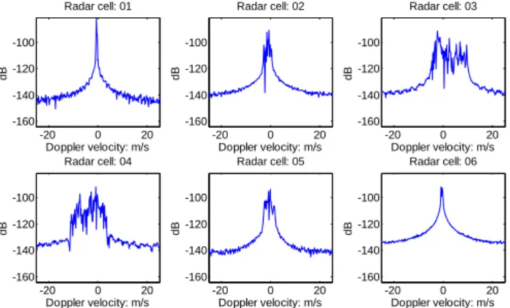
Fig.5. Generation of the initial raindrops (R=1.19mm/h) Figure 6 shows the obtained Doppler spectrum of radar echo in the given 6 radar cells. Here we can easily find that from radar cell 02-05, the width of Doppler spectrum is extended while the width in radar cell 03 and 04 is much wider. Actually this phenomenon is caused by the richness of radial velocities of the scattered raindrops in the given radar cell, as well as the inhomogeneous concentration of raindrops in the wake vortex region. In [2], the Doppler spectrum of wake vortex in clear air was also found to be extended, but with several symmetrical peak values due to its spiral geometry. For radar observation, the radar cells with extended Doppler spectrum indicate the existence of wake vortex. 5. Conclusions

A simulator has been developed for radar monitoring wake vortex in rainy weather. The theoretical derivation for the interaction between raindrops and wake vortex, as well as the interaction between raindrops and electromagnetic waves has been presented. The radar echo model is established for raindrops within wake vortices. The particular shape of the

Doppler spectrum of the raindrops within wake vortices can provide potential information for identifying wake vortex hazard in air traffic control. The current work will be lately improved by taking into account the effect of wind and turbulence on the raindrops' motion.

-20 0 20 -160 -140 -120 -100 Doppler velocity: m/s dB Radar cell: 01 -20 0 20 -160 -140 -120 -100 Doppler velocity: m/s dB Radar cell: 02 -20 0 20 -160 -140 -120 -100 Doppler velocity: m/s dB Radar cell: 03 -20 0 20 -160 -140 -120 -100 Doppler velocity: m/s dB Radar cell: 04 -20 0 20 -160 -140 -120 -100 Doppler velocity: m/s dB Radar cell: 05 -20 0 20 -160 -140 -120 -100 Doppler velocity: m/s dB Radar cell: 06

Fig.6. Doppler spectrum of raindrops in different radar cells Acknowledgements

The first author would like to thank Mr. Florent Christophe (ONERA/DEMR) and Mr. Frederic Barbaresco (THALES AIR OPERATIONS) for their helpful supervisions of this work. This work was partially funded by the THALES Academia program.

References

[1] K. Shariff and A. Wray, “Analysis of the radar reflectivity of aircraft vortex wakes,” J. Fluid Mech, vol. 463, pp. 121–161, 2002.

[2] F. Barbaresco and U. Meier, “Radar monitoring of a wake vortex: Electromagnetic reflection of wake turbulence in clear air, ” C. R. Physique, vol. 11, pp. 54-67, 2010.

[3] T. A. Seliga and J. B. Mead, “Meter-scale observations of aircraft wake vortices in precipitation using a high resolution solid-state w-band radar,” in The 34th

conference on Radar Meteorology, 2009.

[4] J. Li, X. Wang, and T. Wang, “Modeling the dielectric constant distribution of wake vortices,” IEEE

Transactions on Aerospace and Electronic Systems, vol.

47, no. 2, pp. 820 –831, April 2011.

[5] H. Sauvageot, Radar Meteorology, A. House, Ed. Artech House, 1992.

[6] F. Fang, “Raindrop size distribution retrieval and evaluation using an s-band radar profiler,” Master’s thesis, B.S.E.E. University of Central Florida, 2003. [7] T. Gerz, F. Holzpfel, and D. Darracq, “Commercial

aircraft wake vortices,” Progress in Aerospace Sciences, vol. 38, no. 3, pp. 181 – 208, 2002.

[8] S. Lovejoy and D. Schertzer, “Turbulence, raindrops and the l1/2 number density law,” New J. Phys., vol. 10, p. 075017 (32pp), 2008.

[9] B. L. Cheong, R. D. Palmer, and M. Xue, “A time series weather radar simulator based on high-resolution atmospheric models,” Journal of Atmospheric and