Modèles des caractéristiques des branches du pin gris

MODÈLES DES CARACTÉRISTIQUES DES BRANCHES DU PIN GRIS

MÉMOIRE PRÉSENTÉ

COMME EXIGENCE PARTIELLE DE LA MAÎTRISE EN BIOLOGIE

PAR ERIC BEAULIEU

UNIVERSITÉ DU QUÉBEC

À

MONTRÉAL Service des bibliothèques

Avertissement

La diffusion de ce mémoire se fait dans le respect des droits de son auteur, qui a signé le formulaire Autorisation de reproduire et de diffuser un travail de recherche de cycles supérieurs (SDU-522 - Rév.01-2006). Cette autorisation stipule que «conformément

à

l'article 11 du Règlement no 8 des études de cycles supérieurs, [l'auteur] concède

à

l'Université du Québec

à

Montréal une licence non exclusive d'utilisation et de publication de la totalité ou d'une partie importante de [son] travail de recherche pour des fins pédagogiques et non commerciales. Plus précisément, [l'auteur] autorise l'Université du Québec

à

Montréal

à

reproduire, diffuser, prêter, distribuer ou vendre des copies de [son] travail de recherche

à

des fins non commerciales sur quelque support que ce soit, y compris l'Internet. Cette licence et cette autorisation n'entraînent pas une renonciation de [la] part [de l'auteur]

à

[ses] droits moraux ni

à

[ses] droits de propriété intellectuelle. Sauf entente contraire, [l'auteur] conserve la liberté de diffuser et de commercialiser ou non ce travail dont [il] possède un exemplaire.»

REMERCIEMENTS

Je reconnais l'appui financier du CRSNG qui a rendu ce projet possible. Merci à Illon directeur, Frank Berninger, dont l'ouverture et le fiail' m'ont poussé à amener ce projet bien au-delà des ambitions originales. Je suis également reconnaissant du soutien financier qu'il m'a accordé avec lequel j'ai pu m'émanciper davantage grâce à des expériences de terrain et des conférences. Merci à Robert Schneider, un homme de bon conseil, qui a toujours été ·disponible, en particulier à l'aube des étapes critiques du processus d'apprentissage. Je suis reconnaissant de leur apport incontournable et du fait qu'ils m'ont proposé des chemins qui ont conduit au succès. Merci à Tony Zhang, mon co-directeur et Chhun-Huor Ung, un des membres de mon comité d'évaluation, qui ont généreusement partagé leur expertise au profit de ce projet. Merci à tout le monde de la Chaire de recherche en productivité forestière qui m'ont soutenu et aidé à surmonter les obstacles. Je reconnais l'implication d'Isabelle Duchesne et Edwin Swift qui ont collaboré au projet avec le jeu de données du Nouveau-Brunswick. Merci à tous les assistants de terrain qui ont contribué à récolter les données au fil des ans. Merci à tous les autres qui lisent ces lignes.

TABLE DES MATIÈRES

REMERCIElVIENTS . 111

RÉSUMÉ Xl

CHAPITRE l

LISTE DES FIGURES vii

LISTE DES TABLEAUX IX

INTRODUCTION GÉNÉRALE 1

Problématique . . . 1

État des connaissances . . . 4

MODELING JACK PINE BRANCH CHARACTERISTICS 9

1.1 Abstract . . . 10

1.2 Introduction. 11

1.3 Materials and Methods 13

1.3.1 Site Selection .. 13

1.3.2 Tree and branch measurements 14

1.3.3 Model construction. 14

1.4 Results . 19

1.4.1 Number of branches 19

1.4.2 Models for individual branches 24

1.5 Discussion. 30

1.6 Conclusion 36

LISTE DES FIGURES

1.1 Number of branches (nodal and internodal) compared to annual shoot length as a function of annual shoot number . . . . .. 19 1.2 Comparison of distribution for the number of branches (observed) 20 1.3 Distribution for branch insertion angle (observed) . 24

LISTE DES TABLEAUX

1.1 Plot characteristics . . . 15

1.2 Descriptive statistics of branches used for models 18

1.3 Variable abbreviations . 18

1.4 Descriptive statistics for the number of branches (observed) 19

1.5 Coefficient.s for models for number of branches (wit.h SE) 20

1.6 R.andom effects (SD) for models of the number of branches 21

1.7 Prediction errors for models for number of branches 21

1.8 Coefficient.s for insertion angle models (wit.h SE) 24

1.9 Random effects (SD) for brandi insertion angle models . 24

1.10 Prediction errors for branch insertion angle models . 25

1.11 Descriptive statistics for b1'anch diamete1' (observed) 27

1.12 Coefficients for branch diameter models (with SE) 29

1.13 Random effects (SD) for branch diameter models 30

RÉSUMÉ

Quatre-villgt-trois tiges ont été échantillonnécs dans trois régiolls dc l'Est du Ca­ nada de façon à modéliser trois caractéristiques des branches du pin gris: le nombre de branches par pousse annuelle, l'angle d'insertion et le diamètre. Des modèles linéaires généralisés à effets aléatoires ont été privilégiés. Des différences dans les caractéristiques des branches observées entre les branches nodales et internodales nous ont poussés à séparer les modèles par type de branche (nodal versus internodal). Le nombre de branches nodales est proportionnel à la longueur de la pousse annuelle. Le nombre de branches internodales augmente lui aussi avec la longueur de la pousse annuelle, mais diminue avec l'âge de l'arbre. L'angle d'insertion dépend essentiellement du numéro de la pousse annuelle en partant de l'apex (i.e. l'âge de la branche). Les modèles prédisant le diamètre des branches étaient les plus complexes avec la position verticale de la branche et la taille de l'arbre (DHP et hauteur totale) comme groupes de variables explicatives significatives. Les effets aléatoires à l'échelle de la région et de la parcelle étaient infimes par rapport à ceux à l'échelle de l'arbre et de la pousse annnclk. L'importance des effets aléatoires à l'échelle de l'arbre pourrait être un symptôme du contrôle génétique sur le nombre de branches et, dans une moilldre m(~sure, sur le diamètre des bmn<:h~~s. L'in­ teraction entre l'angle d'insertion et le diamètre est relativement forte puisque tous les modèles qui les utilisaicnt montraient de meilleures statistiques d'ajustemcnt, à l'excep­ tion du modèle d'angle d'insertion des branches internodales. Ces résultats nous portent à croire que des variables supplémentaires à l'échelle de l.'arbre, de la pousse annuelle et de la branche devraient être examinées dans l'espoir de mieux comprendre la dynamique des branches.

Mots clés : branchaison, qualité du bois, nombre de branches, diamètre de branche, angle d'insertion de branche, Pinus banksiana

INTRODUCTION GÉNÉRALE

Problématique

La pénurie en bois de sciage dans l'Est du Canada est attribuable à la plus faible disponibilité des espèces traditionnellement utilisées à cette fin. Depuis les années 90, les scieries ont dû s'adapter aux changements en espèces et en dimensions du bois extrait de la forêt (Haygreen et Bowyer, 1989). Parmi ces espèces, le pin gris (Pinus banksiana Lamb.) est le conifère qui croît le plus rapidement au cours des 20 premières années dans son aire de répartition, après le rnélhe laricin (Larix laricina (Du Roi) K. Koch) (Rudolph et Laidly, 1990). On le retrouve principalement dans des peuplements purs, du fleuve Mackenzie dans les Territoires du Nord-Ouest à l'Île du Cap-Breton en Nouvelle-Écosse (Rudolph et Laidly, 1990). Le pin gris représente plus de 20% du volume en résineux au Canada (Law et Valade, 1994) et son bois est utilisé à la fois par les industries du bois d'œuvre et des pâtes et papiers (Duchesne, 2006). C'est aussi la deuxième espèce la plus plantée au Québec (21,3 millions de plants sur 13,2 milliers d'hectares en 2005) (MRNF, 2007).

La densité de plantation des résineux au Québec est passée de 2500 au milieu des années 70 à 1750 plants à l'hectare au milieu des années 90 (Guy Prégent, communication personnelle). Ce changement a été entrepris afin de réduire les coûts de plantation et d'éclaircie, tout en augmentant le diamètre à hauteur de poitrine (DHP) au moment de la première éclaircie et ultimement réduire l'âge de rotation. Cependant, la durée de rotation influence non seulement la rentabilité finandère, mais aussi les propriétés du bois et conséquemment sa qualité et sa valeur (Clark et al., 1996). Les propriétés du bois affectées par un raccourcissement de la durée de rotation sont principalement la résistance et la rigidité en flexion qui diminuent en fonction de la proportion de bois juvénile (Duchesne, 2006).

L'industrie forestière canadienne a maintenu sa position internationale concurrentielle à cause de la disponibilité et le faible coût de la ressource en bois résineux. Au début des années 90, on craignait que cet avantage s'estompe substantiellement (Schuler et Meil, 1D90). Comme cette crainte s'est concrétisée, l'industrie forestière se dirige maintenant vers une gestion intensive pour faire face au problème de la pénurie en bois de sciage. Le pin gris est une espèce propice à la gestion intensive puisque c'est une espèce pionnière dite intolérante à l'ombre qui se développe même sur les sols pauvres. Le problème le plus important avec le pin gris est la taille de ses branches et incidemment des nœuds de son bois qui ont été rapportés comme étant le principal défaut de déclassement (Zhang et aL, 2005). De toute évidence, il existe une relation étroite entre la taille des nœuds et les propriétés mécaniques du bois (Forest Products Laboratory, 1999). Dans ce contexte de gestion intensive, il devient encore plus important de prêter attention à la qualité du bois, en particulier aux causes du déclassement par les nœuds.

La taille et l'angle des branches sont des variables clés parmi les facteurs qui influent sur la forme des nœuds (Lemieux et aL, 1997). Le diamètre et l'angle d'insertion des branches, ainsi que leur djstribution le long de la tige, sont connus comme étant associés aux conditions de croissance de l'arbre tout au long de sa vie. Les branches sont le support des organes photosynthétiques et nous ne pouvons malheureusement les retirer du système! Cependant, le développement plastique des arbres, soit leur capacité à allouer davantage de ressources à la croissance en hauteur ou en diamètre en fonction de la compétition (Govindaraju, 1984), est une occasion pour les sylviculteurs. Les caractéristiques du houppier et des branches peuvent être modifiées par les conditions de croissance (compétition) à travers des pratiques sylvicoles telles que le contrôle de la densité du peuplement, la distribution spatiale des arbres et le choix du site (JVIakinen et Colin, 1998). En fait, l'éclaircie des pinèdes grises résulte en une augmentation du DHP et du volume, mais également de la taille du houppier et du diamètre des branches (Zhang et al., 2006). Par exemple, dans les peuplements de pin gris où l'on a pratiqué l'éclaircie précommerciale de plus grande intensité, les nœuds représentent jusqu'à 50% du déclassement visuel des pièces de bois de sciage de 2 pouces (Zhang et al., 2005).

3

L'éclaircie peut être utilisée pour augmenter la taille des pièces de bois en distribuant la croissance du peuplement à moins d'arbres, ce qui pourrait aider à atténuer certains des problèmes dus à la pénurie d'arbres de grand diamètre. Toutefois, nous avons besoin de rassembler des connaissances plus précises sur les effet.s des t.rai tement.s sylvicoles sur les peuplements de pin gris, en particulier sur leurs effets sur la structure du houppier durant toute la vie de l'arbre, et relier ses caractéristiques à la qualité du bois.

L'approche de plusieurs modèles bases sur les processus repose sur deux principaux pos­ tulats biologiques. Tout d'abord, l'équilibre fonctionnel régit le rapport entre les racines fines et la biomasse foliaire. Ensuite. le bilan hydrique et de la structure mécanique sont présentés par le rapport entre la surfa.ce d'aubier et la biomasse foliaire (1tHikeHi, 1997). Ce dernier postulat est connu comme la théorie du modèle tubulaire qui est basé sur la relation entre la section transversale des organes non photosynthétiques à une hauteur donnée et la quantité de feuillage de ce niveau jusqu'à l'apex (Shinozaki et aL, 1964). Comme l'a mentionné Makeli:i (2002), le rapport feuillage sur surface d'aubier a par la suite été étudiée dans le contexte d'une relation avec la conductivité de l'eau dans le tronc. Cette théorie a été adaptée pour fonctionner de manière dynamique dans un cadre de bilan du carbone.

Le développement du houppier diffère d'arbre en arbre selon l'idée que les arbres allouent leurs ressources en fonction de la disponibilité de l'environnement de lumière et/ou de l'espace physique. Un arbre en croissance libre croît avec un minimum d'auto-élagage, tandis qu'un arbre faisant face à ulle forte compétition se développe en hauteur autant que possible.

Plus récemment, ces modèles ont été utilisés en conjonction avec des modules de qualité du bois afin d'évaluer les effets des choix d'aménagement sur la croissance du pin syl­ vestre (Miikelii et Miikinen, 2003). Étant donné que cette méthode d'évaluer la qualité du bois s'est révélée être un succès (Makelii et Miikinen, 2003; Kantola et aL, 2007) et que le pin gris ressemble au pin sylvestre à divers égards, cette approche a été considérée comme la plus prometteuse dans notre contexte. En fait, la validation préliminaire de

Crobas pour le pin gris a montré des résultats prometteurs.

L'objectif de cette étude est de développer des modèles pour trois déterminants de la qualité du bois, soit le nombre de branches, leur angle d'insertion et leur diamètre pour chaque verticille à l'aide de variables des échelles supérieures (verticille, arbre et peuplement).

État des connaissances

Modélisation des arbres

Pour modéliser la croissance des arbres, nous nous basons sur les connaissances acquises sur les interactions de chacune de ses composantes avec son environnement. Les ob­ servations faites sur la forme des arbres nous ramènent à Leonard de Vinci qui a noté que le diamètre cumulé de toutes les branches d'un arbre à une hauteur donnée est égal au diamètre du tronc (Aratsu, 1998). La théorie du modèle tubulaire précise cette observation avec la. retati9n directe. entre la superficie -d'aubier à une hauteur donriée ­ et la biomasse foliaire au-dessus de cette hauteur (Shinozaki et aL, 1964). Le concept peut être vu comme un tuyau reliant chaque unité de feuillage à son système racinaire respectif. Cette relation est de manière générale véridique, mais elle a toujours été une notion morphologique limitée (Sievanen et aL, 2000).

Les modèles structure-fonction ont été développées plus récemment, en réponse à la nécessi té d'examiner les processus physiologiques et leurs interactions avec l'environne­ ment (à l'extérieur et à l'intérieur de l'arbre), avec la même précision (Bosc, 2000). L'un d'eux intègre à la fois le fondement théorique du concept de modèle tubulaire et des mo­ dules de qualité du bois. Ce modèle, appelé PipeQual, c:onccpt1li'1lise les arbres comme des organismes stlllcturés qui peuvent être divisées en trois niveaux principaux: la tige, les branches et le feuillage (Makela et Makinen, 2003). Ces trois niveaux sont pertinents dans l'analyse des échanges entre les composants: l'arbre qui interagit avec l'environ­ nement, les verticilles qui répartissent les ressources entre le tronc et les branches et les

5

branches qui supportent le feuillage où se produit la photosynthèse. En dépit de l'uti­ lisation de trois échelles différentes, la plupart des équations impliquent des variables du niveau de l'arbre. Toutefois, il est généralement bien établi que les branches sont af­ fectées dans leur croissance par l'intensité de la compétitioll, souv(·mt associée à l'ombre projetée par le houppier des compétiteurs. Seules quelques études ont réussi à identifier l'ampleur de l'exactitude cie cette relation. Par exemple, Makinen et Colin (1998) ont utilisé un indice de compétition dépenclant de la distance afin de quantifier comment la carence en lumière influence la croissance des branches.

Des efforts ont également été faits par cles auteurs tels que Bosc (2000) avec le moclèle EMILION qui est basé sur des processus reliées au carbone et à l'eau et leurs interactions aux échelles cie l'organe et de l'arbre. Élaborés pour des espèces de pin, ce modèle a montré qu'en vieillissant, les branches deviennent autonomes et ne contribuent que faiblement au fonctionnement global cie l'arbre. Comme il n'y a pas plus beaucoup de carbone disponible, leur développement est limité et lorsque l'équilibre de carbone s'affaiblit la branche finit par mourir.

Relations du houppier et des branches

Avant le début cie la seconde moitié du 20e siècle, la forme du houppier était interprété en fonction du concept de dominance apicale. La dominance apicale est le contrôle exercé par le sommet de la pousse annuelle sur le débourrement des bourgeons latéraux (Cline, 1997). Cette théorie influente est parvenu à expliquer les différences de structure de houppier entre les espèces, en particulier entre la ramification excurrente cie la plupart des espèces cie conifères et déliquescente de la majorité des espèces cie feuillus (Brown, 1971). La forme conique dn houppier des conifères est expliquée par un contrôle apical fort, tanclis que la forme ronde des essences feuillues dénote un contrôle apical faible (Cline, 1997). Les conifères ont ainsi tendance à allouer davantage de ressources à la flèche et moins aux branches plus basses, faisant de l'auto-élagage une caractéristique inhérente à ces arbres.

L'intérêt pour la modélisation des branches s'est intensifié dans les années 90. Dans un premier temps, les travaux ont été consacrés à l'impact de la provenance sur la structure du houppier et les résultats présentés étaient plutôt descriptifs. Peu après, des modèles de caractéristiques des branches ont été développés. La modélisation des branches des conifères a été essentiellement effectués sur les principales espèces croissant en Europe, comme Pinus sylves tris (Makela et aL, 1997; Petersson, 1998; Makinen et Colin, 1998; Kellomaki et aL, 1999; Makinen et Colin, 1999; Makinen, 1999b,a; Makela et Vanninen, 2001; Makinen et Makela, 2003; MakeUi et Makinen, 2003; Ulvcrona et aL, 2007) et Picea abies (Colin et Houllier, 1991; Colin et aL, 1993; Houllier et aL, 1995; Loubère et aL, 2004; Kantola et aL, 2007; Hein et aL, 2007). D'autres travaux moins récents traitent de la branchaison de Picea sitchensis (Cochrane et Ford, 1978), Pseudotsuga menziesii (Kershaw et Maguire, 1990; Maguire et aL, 1994; Maguire, 1994; Maguire et al., 1999; Briggs et al., 2007), Pinus nigra (Matziris, 1989; Meredieu et aL, 1998), Pinus taeda (Doruska et Burkhart, 1994), Pinus radiata (Woollons et al., 2002) et Pinus banksiana (Morris et aL, 1992).

Cinq variables principales ont été modélisées dans la littérature portant sur les branches par rapport. à la qualit.é du bois: 1) le nombre t.ot.al de branches, 2) h~ nombre d(~

branches par verticille, 3) le diamètre des branches, 4) l'angle d'insertion des branches et 5) l'azimut des branches à l'intérieur du verticille.

Le nombre total de branches que portent un arbre est la conséquence des conditions de chacune des saisons de croissance auxquelles il a fait face. Dans la littérature liée à la modélisation des branches, seules quelques études ont utilisé le nombre total de branches comme un moyen cie comprendre l'influence générale du contrôle génétique et de l'environnement sur la branchaison. Doruska. et Burkhart (1994) ont lié le nombre total cie branches vivantes à l'intérieur du houppier à la longueur du houppier pour le pin à encens (Pinus taeda). Le nombre de branches vivantes (par tranche de 1 m de long) a été lié à la distance de l'apex (Miikinen et. al., 2003). Un autre moyen de se concentrer sur le nombre total de branches est par le biais du nombre de verticilles qui dépend du DHP et de la longueur du houppier (Doruska. et Burkhart, 1994). Toutefois,

7

le nombre de branches est généralement modélisé à l'aide de la croissance en hauteur car c'est une variable qui synthétise une série de variables environnementales, tel que la longueur de la saison de croissance. Plus la saison de croissance est longue, plus l'accroissement en hauteur de J'arbre est grand et plus le nombre de branches d'une pousse annuelle donnée est élevé (Colin et al., 1993). En effet, de nombreux auteurs se sont appuyés sur l'incrément en hau teur afin de prédire le nombre de branches par pousse annuelle (Houllier et al., 1995; Miikelii et al., 1997; Miikinen et Colin, 1999; Miikelii et Makinen, 2003; Kantola et al., 2007; Hein et al., 2007). Colin et al. (1993) ont montré que le nombre de branches internodales diminue avec la distance de l'apex, donc que la variabilité du nombre de branches par pousse annuelle peut être expliqué, du moins en partie, par le numéro de l'unité de croissance (à partir cie l'apex). Les branches nodales marquent la fin de la saison de croissance, tandis que les bourgeons internodaux sont dormants la première année et débourrent l'année suivante. Ceci suppose que le nombre de branches nodales dépend de la longueur de la saison cie croissante courante et que le nombre cie branches internodales des conditions de la suivante. La compétition n'a pas d'effet significatif sur le nombre de branches sur la flèche. De faibles relations avec le rapport hauteur/diamètre (Miikinen et Colin, 1999; Hein et al., 2007), la hauteur de l'arbre, le DHP (Miikelii et Miikinen, 2003) et l'âge de l'arbre (Kantola et al., 2007) ont été ajoutées aux modèles du nombre de branches par pousse annuelle.

Le diamètre des branches est évidemment la variable la plus importante dans l'évaluation de l'impact des nœuds sur le déclassement du bois. Le diamètre des branches à l'insertion dans le tronc correspond à l'extension latérale du houppier et dépend du statut social et de l'historique de la densité du peuplement (Colin et aL, 1993). Le diamètre des branches a été lié à la distance de l'apex, la hauteur de tige, le DHP et à la longueur relative du houppier (Colin et al., 1993; Houllier et al., 1995; Miikinen et Colin, 1998; Meredieu et al., 1998; Loubère et al., 2004). En raison de l'impact des gros nœuds sur la qualité du bois, le diamè~re de branche maximal par verticille a souvent été la variable privilégiée. Il est principalement dicté par le DHP et la profondeur dans le houppier (Maguire et al., 1991; Doruska et Burkhart, 1994; Maguire et al., 1999; Miikinen et

Miikelii, 2003; Miikinen et al., 2003; Hein et al., 2007). La croissance des branches les plus hautes dans le houppier est plus dépendante des facteurs régionaux tels que le climat, tandis que les branches inférieures du houppier sont grandement affectés par des facteurs locaux comme la compétition (Miikinen, 1D99a).

L'angle d'insertion des branches est principalement liée à la distance de l'apex, le numéro de la pousse annuelle (à partir de l'apex) et le DHP (Colin et al., 1993; Houllier et al., 1995; Miikelii et al., 1997; Miikinen et Colin, 1998; Meredieu et aL, 1998; Miikinen et Miikelii, 2003; Miikinen et al., 2003; Kantola et al., 2007). D'autre part, il existe une relation étroite entre le diamètre et l'angle d'insertion (Houllier et al., 1995), qui est forte pour le pin gris (Drolet et al., 1971). 'L'angle d'insertion des branches vivantes du pin gris (diamètre supérieur à

1

pouce) est en moyenne de 70 degrés (écart type de 16) (Drolet et al., 1971). Les branches ont tendance à s'affaisser après les premières années de croissance pour Picea abies, Pinus sylves tris et plusieurs variétés de Populus (Franklin et Callaham, 1970). L'angle d'insertion d'une branche dépend du poids qu'elle soutient toute sa vie, à la fois de sa propre biomasse et des précipitations (Colin et al., 1993).

Seules quelques études ont traité de l'azimut de branches parce qu'on assume que les branches sont espacées régulièrement dans le verticille, sans agglomération systématique (Doruska et Burkhart, 1994; Miikelii et al., 1997; Miikelii et Miikinen, 2003; Kantola et al., 2007), Toutefois, Lemicux et al. (1997) ont examiné la forme et la distribution des nœuds sur la surface de sept billes d'épinette de Norvège et leurs résultats montrent une concentration des branches au sud-est. Les branches du côté sud ont une croissance supérieure (Bjorklund, 1997; Lemieux et al., 1997, 2002). De plus, on a observé une nombre de branches vivantes plus grand et de plus grosses branches au sud-ouest pour le pin gris (Drolet et aL, 1971) et au sud pour l'épinette de Sitka (Achim et aL 2006). L'azimut des branches pourrait alors être utile pour l'optimisation de la qualité du bois par la rotation appropriée du bois de sciage (Lernie\\x et al., 2000; Benjamin et al., 2007).

CHAPITRE l

MODELING JACK PINE BRANCH CHARACTERISTICS

Eric Beaulieu*, Robert Schneider*, Frank Berninger*, Chhun-Huor Ung

t

and Edwin Swift§

* Département des Sciences biologiques, Université du Québec à Montréal, C.P. 8888, succursale Centre-Ville, Montréal, QC H3C 3P8, Canada.

t Natural Resources Canada, Canadian Forest Service, Canadian Wood Fibre Centre, P.O. Box 13080, Ste-Foy, Québec, QC G1V 4C7, Canada.

§ Natural Resources Canada, Canadian Forest Service, Canadian Wood Fibre Centre, Atlantic Forestry Centre, P.O. Box 4000, Fredericton, NB E3B 5P7, Canada.

A total of 83 trees were sampled in three regions of Eastern Canada in order to model branch characteristics (number of branches per annual shoot, branch insertion angle, and diameter). Generalized mixed-effect linear models were used to do so. Differences in branch characteristics according to branch type were also studied. The number of nodal branches is proportional to the annual shoot length. The number of internodal branches also increases with annual shoot length, but decreases with tree age. Insertion angle was mainly driven by annual shoot number from apex (branch age). The diameter models showed the most complexity with branch vertical position and tree size (DBH and total height) as groups of variables statistical!y significant. Region and plot random effects were minimal cornpared to the tree and annual shoot levels. Tree-Ievel random effects were significant for every model and might be a symptom of genetic control on the number of branches and to a smal! extent branch diameter. Interaction between insertion angle and diameter is relatively strong, because al! the models using them as independent variables (except for the model of insertion angle fOF-internodal branches) showed better fit statistics. These results lead us to believe that tree-, annual shoot- and branch-Ievel variables should be further explored in order to better understand branch dynamics.

Keywords : branchiness, wood quality, number of branches, branch diameter, branch insertion angle, Pinus banksiana

1.2 Introduction

Jack pine (Pinus banksiana Lamb.) is the second most planted species in the province of Quebec (MRNF, 2007) and is the fastest-growing conifer during the fast 20 years in its native range, other than tamarack (Larix laricina (Du Roi) K. Koch) (R.udolph et Laidly, 1990). More and more pine stands are established as plantations and their management is gradually changing. The softwood plantation density in Quebec was decreased from 2500 stems ha-I _{in the mid 70}/S

to 1750 stems ha-I _{in the mid 90}/S due to decreased post-plantation mortality and in order to increase the prafitability of future thinnings (Guy Prégent, personal cOIIlIIltmication). This change could however significantly reduce wood quality. Previous studies have shown that the most serious problem with jack pine wood quality is branch size, where lmots have been reported as the main lumber downgrading defect (Zhang et aL, 2005). It is well known that knot size depends on stand density and methods are needed to understand how stand density and other factors interact on knot properties.

Under natural conditions, jack pine regenerates typically in pure dense stands after fire. Growing fast in the first few years, the lowest branches are generally self-pruned. This naturally prevents a great impact on the most valu able part of the lumber since branches and the resulting knots remain relatively small. In density controlled environments such as plantations or after pre-commercial thinning, branches are however more persistent and might grow more rapidly. Crowns may then vary from a clear, long and conic-shaped in free-to-grow environments to short and compact in dense stands, and ta a neglected aspect in harsh soil and drainage conditions (Farrar, 1995). Another property of this species is the presence of internodal branches, i.e. branches formed along the annual shoot as opposed to nodal branches which are found at the top end of the annual shoot. The only strong indicator of the number of branches pel' growth unit is the annual shoot length that synthesizes both the site and environmental growing conditions. The number of branches is known to be proportional to height increment and inversely proportional to tree age (Kantola et al., 2007). However, since height increment decreases with tree

age, it becomes hard to explicitly differentiate both. Density could also have an effect on the number of branches (Miikinen et Colin, 1999) but the link is not clearly established (Briggs et aL, 2007). However, heightjdiameter ratio, a measure of competition that is rnainly controlled by density, was found to influence the number of branches per unit length (Miikinen et Colin, 1999). Studies of understory balsam fir showed that both the apical dominance ratio and the number of branches increase with light availability (Parent et Messier, 1995; Duchesneau et aL, 2001). The number of branches is also believed to be partly determined by genetic control (Vest01 et al., 1999).

Only a few studies showed results with an emphasis on branch type for species with internodal branches. For Sitka spruce, the number of internodal branches is greater than that of the nodal branches in the top half of the tree (Achim et al., 2006). Below the mid-point of the stem, the number of internodal branches decreases more rapidly than the nodal branches.

Branch insertion angle has been mainly related ta the distance from the apex, the annual

sn6ôriiU-moer--Cstartlngffom-tneaJfex-)";-anof)'!31I fCoti·n-et--at-;-1§9'3";-HoU"iiieret-at-l.-,- - - ­ 1995; Miikelii et aL, 1997; Miikinen et Colin, 1998; Meredieu et aL, 1998; Miikinen et

Miikelii, 2003; Miikinen et aL, 2003; Kantola et al., 2007). On the other hand, there is a close relationship between diameter and insertion angle (Houllier et al., 1995). Branches have the tendency to flatten out after the first few years of growth for Picea abies, Pinus sylvestris, and for several Populus varieties (Franklin et Callaham, 1970). Insertion angle depends on both the branch biomass and the precipitations it supports during its lifespan (Colin et aL, 1993). Insertion angle tends to decrease with age as its biomass increases and pushes it down under gravity. There is also an opposing force advantaging the growth of branches with acute angle with respect to stem that usually have easier access to light (Samson et al., 1996; Wilson, 2000).

Branch diameter was found to depend on social status and stand density history (Colin et al., 1993). It has been related to the distance from the apex, stem height, diameter at breast height (DBH), and crown ratio (Colin et al., 1993; Houllier et aL, 1995; Miiki­

13

nen et Colin, 1998; Meredieu et al., 1998; Loubère et al., 2004). Because of the impact of large knots on wood quality, maximum branch diameter within a whorl has often been the preferred variable. It is mainly dictated by DBH and crown depth (Maguire et al., 1991; Doruska et Burkhart, 1994; Maguire et al., 1999; Makinen et Makela, 2003; Makinen et al., 2003; Hein et al., 2007). The growth of branches higher in the crown is more dependent of site factors such as climate and site fertility, while branches lower in the crown are largely affected by local factors such as competition (Makinen, 1999a). Increasing stand density hasten the thinning of rings and death of the branches (Maki­ nen, 1999a). Achim et al. (2006) found that nodal branches are larger than internodal branches.

The objective of the paper is to study the relationships between certain branch charac­ teristics (number of branches pel' annual shoot, branch insertion angle and diameter) and branch, tree and stand variables. Generalized mixed-effect linear models are used to model these variables.

1.3

Materials and Methods

1.3.1

Site Selection

Naturally regenerated and planted jack pine stands were sampled in three sites in Eas­ tern Canada: Petawawa Research Forest (Ontario), Smurfit-Stone freehold (Quebec), and Eel River Bridge (New Brunswick). Stands were mostly on deposits of outwash, fluvial, and aeolian origin with a few tiUs. Soils were mostly sandy textured podzols and drainage varied from good to excellent. The sites were chosen as to obtain a variety of representative combinations of stand density, age, and site indices (SI). Density ranged from 583 to 3850 stems ha-l, age from 21 to 79 years old, and SI (at 20 years of age) from 5.9 to 14.0 m (Table 1.1). More specifically, the Ontario site was an initial spacing trial composed of 2 different spacings : 7' and 14' spacing. The Quebec sites were com­ posed of operational plantations ranging in age from 21 to .37 years and in density from 1775 to 3850 stems ha-1. Naturally regenerated, untended stands were also sampled

-

--with the following characteristics : 61 to 79 years old, 2075 to 2625 stems ha-1 and 6.5 to 9.5 m in Sr. The Eel River Bridge site was precommercially thinned at age 16 (Zhang et al., 1998). The 4', 7' and 9' spacings were sampled. Stand and tree characteristics at time of sampling can be found in Table 1.1. For ail sites, stand conditions before thinning were assumed to have no effect on the branch characteristics within the crown due to the long time that had passed since thinning.

1.3.2 Tree and branch measurements

Sample tree selection is detailed in Schneider et al. (2008a). In summary, diameter at breast height (DBH) of ail the live trees in the plots was measured and they were cored at breast height to calculate annual DBH increment. The DBH distribution was then divided into 3 equally sized classes, and at least one sample tree per size class was randomly selected in the stand. After felling, total stem height and height to live crown base, defined as the lowest live nodal whorl (containing at least one live branch) not separated by the main crown by more than one dead whorl, were noted. The height of every whorl was recorded and identified as nodal or internodal. Nodal branches are at the top of each annual shoot, while internodal branches are generally smaller branches along the internode (between nodal whorl of a given year and previous year). Branch measurements included whorl type, whorl height, stem diameter at whorl base, state (deadjalive), the diameter at the base of the branch (above the swell, about 5 cm from the insertion point), and insertion angle (with 90° being the horizontal). A summary of the descriptive statistics of data used to build the models is compiled in Table 1.2. Ail abbreviations for the variables used in the models are enumerated in Table 1.3.

1.3.3

Model construction

A few steps were required to come to the final models presented in this study. First, a stepwise linear regression was used as to identify the most important independent variables. Second, these variables were tested in a mixed-effects model with region, plot, tree, and annual shoot random effects applied on the intercept. The most non-significant

15

Tableau 1.1 Plot characteristics

Plot Stand Density

G

DBH Site Index

_#

Age (ha-1_{) (m}2 _ha-1₎ (mm) (H20 , m) (years) Ontario 1 1441 38.7 185.0 14.0 10 41 3 583 28.8 251.0 14.0 6 41 Québec 51 2032 11.1 83.4 7.8 3 21 52 2159 20.9 110.9 9.2 3 22 53 2200 24.2 118.3 9.3 3 22 54 1775 ]5.2 104.5 9.2 3 22 56 2150 ]1.6 83.0 6.7 3 21 58 2925 13.6 76.9 8.3 3 21 59 3850 11.0 60.3 6.1 3 22 60 2850 12.5 74.7 6.6 3 21 64 3225 12.0 68.9 6.7 1 24 65 2275 19.9 105.5 10.4 3 21 66 2325 22.9 112.1 5.9 3 37 67* 2275 24.1 116.1 7.0 3 79 68* 2075 29.7 135.0 9.0 3 77 69* 2625 39.5 138.4 9.5 3 79 70* 1400 24.2 148.2 9.5 3 61 71* 1850 25.5 132.4 8.0 3 59 72* 2350 18.4 99.8 6.5 3 62 New Brunswick 102* 3150 39.2 125.8 9.0 6 56 104* 2200 40.4 153.0 9.0 6 56 105* 2175 20.2 108.7 9.0 6 56

* : Natural regeneration, G: Stand Basal Area,

variable was removed iteratively until only significant variables were left, as proposed by Littell et al. (1996). Third, different combinations of transformations were tested. Ail hierarchal level random effects were initially added, with the non-significant levels deleted in the final models. R.andorn efi"ects were then tested in interaction with the independent variables.

Generally, whorl type was used as a segregation factor, with the nodal and internodal branches being modeled separately. The models predicting branch insertion angle and branch diameter were estimated using linear mixed-effects regressions, and the models for the number of branches used a mixed-effect Poisson regression. On an annual shoot, there is always one nodal whorl and 0 to n internodal whorls. For the model of the number of internodal branches, the number of internodal whorls was tested as an inde­ pendent variable. The Poisson regressions use ail the branches (live and dead) located above the live crown base.

Insertion angle and branch diameter were modeled using a linear mixed-effect model as previously described. Since these variables have been reported to be strongly related, ­ two types of models were developed. For branch insertion angle, a first model was tested without branch diameter, and a second model with branch diameter included in the list of independent variables. The same was done for branch diameter, where one model used the insertion angle and the second without. Ail live branches ab ove live crown base were used for these models.

Random effects were examined at region, plot, tree, and annual shoot levels. Ail of the models were calibrated using the Ime (Pinheiro et aL, 2008) and lmer (Bates et aL, 2008) procedures in R, respectively for models of the number of branches and models for individual branches (insertion angle and diameter). Model -valuation ,vas done using residual plots and the Akaike information criterion (AIC), the Baysian information criterion and the log-likelihood (Pinheiro et Bates, 2000). Lastly, three model prediction errors were used in characterizing each model (Makinen et Colin, 1999). These were the mean error (Eq. 1.1), the absolute mean error (Eq. 1.2), and the mean square error (Eq.

17

1.3) :

E =

l:)y -

y)/n

(1.1 )

lEI

=

L

Iy -

yl/n

(1.2)

Tableau 1.2 Descriptive statistics of branches used for models

AU Ail branches Ali live branches

branches above crown base above crown base

Region

_#

NBT* NNB NIB D (mm) lA

n

Ontario 16 365.8 (34.7) 4.4 (1.7) 5.6 (3.9) 11.3 (9.2) 59.2 (16.4) Québec 49 244.2 (46.5) 4.0 (1.6) 2.5 (2.9) 8.7 (6.6) 69.9 (19.1) NB 18 366.5 (29.4) 3.7 (1.4) 2.9 (2.5) 9.5 (7.2) 69.3 (17.9) Ali 83 294.2 (39.0) 4.0 (1.6) 3.1 (3.1) 9.4 (7.4) 67.4 (18.8)

* :

Number of branches per tree (% green), # : Number of Sam pIe Trees, NB : New Brunswick

Tableau 1.3 Variable abbreviations

NNB Number of nodal branches lA Insertion angle

n

NIB Number of internodal branches D Diameter (mm)

ASL Annual shoot length (cm) RHWC Relative height within crown (%)

DI Diameter increment at BH (mm) HB Height to branch (cm) TH Tree total height (cm) RH Relative height (HB/TH) NIW Number of internodal whorls DBH Diameter at breast height (mm) ASNFB Annual shoot number from base WNFA Whorl number from

apex

ASNFA Annual shoot number from apex HCB Height to crown base (cm)

N and IN Nodal and internodal

le

lntercept

SE and SD Standard error and standard deviation Random effect

Residual error

••• ••••• •

1.4 Results

1.4.1

Number of branches

100 '0 4.5

• •

o

...

• 80 ••• ~ ~ ·0

o·.... ..

.

• o 0 ~ ~ • 0 0 ° ° 0 0 0 • • • • • • • 10 • o 0 o • • _{••••••} 3.5 o 00 • 0 00 0 •

.

...

•

• • o 00

• •

••• 60 0 0 0

.

..

..

0 0 o • 2.5 10 20 '0 o1--- - - _ - - _ - - _ - - ~ - - ~ - - _ - - _ -_ __I_o o 10 20 JO 10 50 GO 70 80 90

Annual Shoot Numbe. !rc:~ UëI$e

OAnnu",l shoot L.~n9th eNu."!tber oC Nodal (jranches ONu:nber oC Internodllll Ul.n.ehes

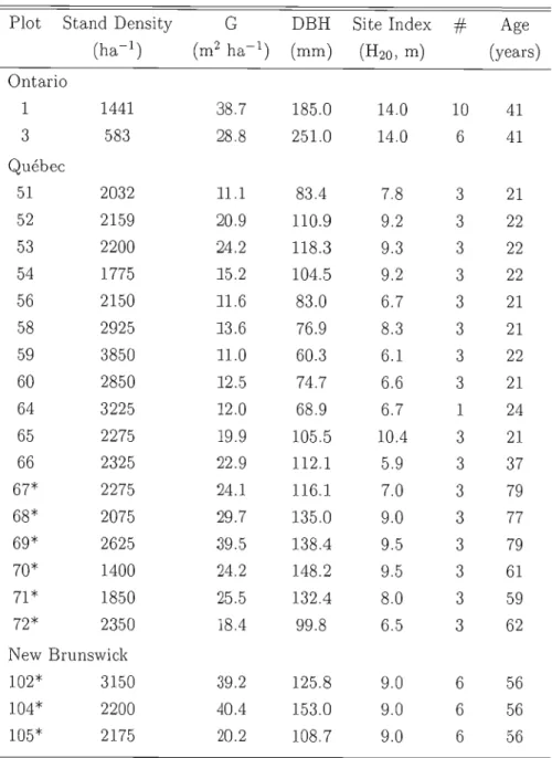
Figure 1.1 Number of branches (nodal and internodal) compared to annual shoot length as a function of annual shoot number

Tableau 1.4 Descriptive statistics for the number of branches (observed) Min. 1st Qu. Median Mean Mode 3rd Qu. l\tIax. SD CV

N 1 3 4 4.0 3 5 20 1.6 40%

IN 0 0 3 3.1 0 5 22 3.1 100%

SD : Standard Deviation, CV Coefficient of Variance (SDjMean)

Number of nodal branches

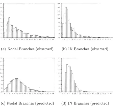
The mean number of nodal branches produced each year is rather constant throughout tree life (Figure 1.1) as it is shown by a lower variation coefficient (standard deviation

j mean) of 40% than that of the number of internodal branches (Table 1.4). A period of the first 40 years of tree life starts from and finishes with the production of almost

1 l ~ 7 • Il IJ l~ P l? O ! ~ ~ • 10 l~ 1( H Il d. 27.

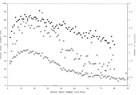
(a) Nodal Branches (observed) (b) IN Branches (observed)

,,,

..

_n

0' ,- h

(c) Nodal Branches (predicted) (d) IN Branches (predicted)

Figure 1.2 Comparison of distribution for the number of branches (observed)

4 branches, and peaks to a little less than 5 inbetwëen (Figure 1.1). After 40 years, a slight decrease is then observed to a minimum of a little less than three branches for the oldest whorls. The frequency distribution of the number nodal branches resembles that of a normal distribution whereas that of the internodal branches is more of inversed J-distribution (Figure 1.2). Frequencies in the lowest classes are overestimated by the model of the number of internodal branches.

Tableau 1.5 Coefficients for models for number of branches (with SE)

Model aO (IC) al (L) a2 (DI) a3 (NIW) a4 (HB) a5 (ASNFB) NNB 0.6763 0.1928 0.1266

(Eq. 1.5) (0.0637) (0.0220) (0.0207)

NIB -1.4974 0.8853 0.2926 -0.0171

21

Tableau 1.6 Random effects (SD) for models of the number of branches

Model Plot Tree AnnualShoot

(cx rp ) (cxrpt) ( CXrpta)

NNB (Eq. 1.5) IC 0.0267

NIB (Eq. 1.7) IC 0.3291 0.5430 0.3453 NIB (Eq. 1.7) NIW 0.1987 0.2128 0.2561

Tableau 1. 7 Prediction errors for models for number of branches

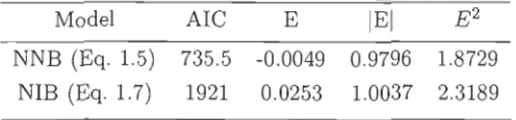
Model AIC E

lEI

NNB (Eq. 1.5) 735.5 -0.0049 0.9796 1.8729 NIB (Eq. 1.7) 1921 0.0253 1.0037 2.3189

The number of nodal branches was modeled using a mixed effect Poisson regression

(1.4)

where

(1.5)

- ao

to a2 fixed effect pal'arneters

~ CXrpt tree-level random effect, where CXrpt "-' N(O, a;pt)

The model shows that the number of nodal branches is proportional to both annual shoot length and DBR increment (Table 1.5). The importance of the an nuaI shoot length is greater than that of diameter increment. Finally, the only significant random effect is at tree level (Table 1.6). The

lEI

error is close to 1 and similar to the result for the model for internodal branches (Table 1.7).

N umber of internodal branches

The number of internodal branches follows the same trend as that of the annual shoot length wi th regards to shoot age (Figure 1.1). In the first 20 years, both the number of

internodal branches and shoot length increases until it reaches its maximum. Thereafter, both decrease. Nevertheless, the major difference compared to the number of nodal branches is a higher coefficient of variation of 100% (Table 1.4). As trees get older, the , proportion of internodal branches on annual shoot decreases.

23

As with the number of nodal branches, the number of internodal branches was modeled using mixed efl'ect Poisson regression.

NI B rpta ev POiS(ÀN JB) (1.6)

where

ÀN JB

=

aü

+

a3 ln (N IWrpta )

+

a4 ln (H Brptaw)

+

asA5NF Brpta

+

Ctrp

+

Ctrpt

+

Ctrpta

+

CtrpN JW . ln (N IWrpta ) (1. 7)

+

CtrptN JW . In(NIWrpta )

+

CY,ptaN JW . In(NIWrpta )

- aü to as are fixed efl'ect parameters

- Ctrp , Œrpt, Œrpta, O'rpNJW,O'rptNJW and ŒrptaNJW are random efl'ects, where:

- Œrp ev N(O, a-;p)

- Ctrpt ev N(O, a-;pt)

- O'rpta ev N(O, a-;pta)

- CtrpNJW ev N(O,a-;pNJW)

- CtrptNJW ev N(O,a-;ptNJW)

- CtrptaN JW ev N

(0, a-;ptaN JW )

The model shows that the number of internodal branches is proportional to both annual shoot length and the height of the tip of anoual shoot and is inversely proportional to the annual shoot number from base. As with the model to predict the number of nodal branches, the logarithmic transformation of annual shoot length greatly improved the model. Random efl'ects were significant at alllevels apart from region (Table 1.6). This is the only mode! where a random efl'ect is applied to an independent variable, in this case NIW. The errors are ail worse than for the model for nodal branches, especially for E2 that is over 2 (Table 1.7).

Figure 1.3 Distribution for branch insertion angle (observed)

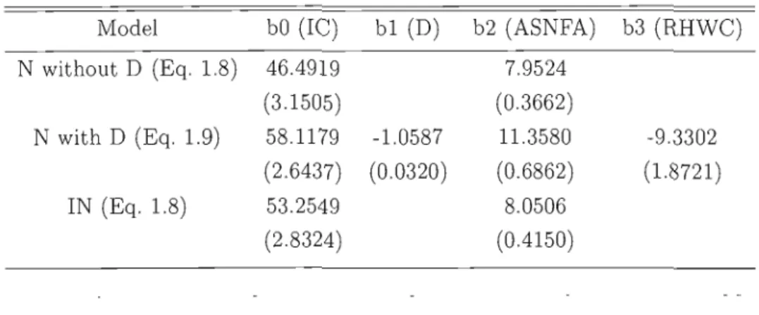
Tableau 1.8 Coefficients for insertion angle models (with SE)

Model bO (IC) b1 (D) b2 (ASNFA) b3 (RHWC) N without D (Eq. 1.8) 46.4919 7.9524 (3.1505) (0.3662) N with D (Eq. 1.9) 58.1179 -1.0587 11.3580 -9.3302 (2.6437) (0.0320) (0.6862) (1.8721) IN (Eq. 1.8) 53.2549 8.0506 (2.8324) (0.4150)

1.4.2

Models for individual branches

Insertion angle

Insertion angle is fairly normally distributed with the only particularity of a break after 90· class (Figure 1.3). Branches of more than 90' represent 4.8% of the nodal branches and 5.8% of the internodal type. Mean insertion angle of nodal and internodal branches is 66.0· and 69.2·, respectively. The difference is small however, it was found during model

Tableau 1.9 Random effects (3D) for branch insertion angle models

Model Region Plot Tree AnnualShoot Residual

ïvIodel (CYr) ( CY rp ) (CYrpt) ( CYrpta) ( érpta)

N without D (Eq. 1.8) 5.0310 0.0188 7.1869 5.0389 15.3877 N with D (Eq. 1.9) 0.0063 2.1804 7.4215 5.6774 13.7274

25

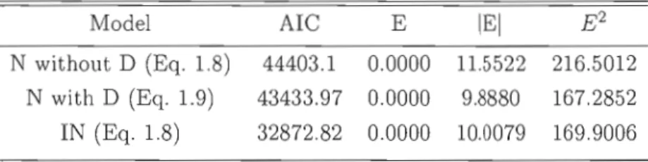
Tableau 1.10 Prediction errors for branch insertion angle models

Model AIC E

_lEI

E 2

N without D (Eq. 1.8) 44403.1 0.0000 11.5522 216.5012 N with D (Eq. 1.9) 43433.97 0.0000 9.8880 167.2852

IN (Eq. 1.8) 32872.82 0.0000 10.0079 169.9006

construction that the internodal variable was significant. Therefore, it was decided to build separa te models for nodal and internodal branches. Linear mixed-effect models are used to relate insertion angle to the different independent variables. Moreover, models were built with (Eq. 1.9) and without (Eq. 1.8) branch diameter.

Two equations encompass the four model options for the prediction of insertion angle:

l Arptawb = bo

+

b2 ln(ASNFA rpta )

(1.8)

+O:r

+

cxrp

+

CXrpt

+

CXrpta

+

érpta

( 1.9)

+CXr

+

cx rp

+

CXrpt

+

CXrpta

+

érpta

where

- bo to b3 are fixed effect parameters

- CX r , cx_{rp , CXrpt} and CXrpta are randorn effect.s, where :

- CX r '" N(O, a;)

- cx rp '" N(O, a;p)

CXrpt'" N (0, a;pt)

- CXrpta '" N(O, a;pta)

- Erpta is the model error, where Erpta '" N(O, a 2)

The model of insertion angle is straightforward with one significant covariate in ail four model options (Table 1.8). The insertion angle is proportional to branch age (ASNFA). The branch diameter was significant only for the model for nodal branches where it improved the AIC, whereas no other variable was found significant for the internodal branches. Nodal branches tend to bend down as they get bigger (D) and deeper within crown (RHWC). For models not including diameter as a significant covariate bO and b2 were higher for internodal branches. The intercept and the coefficient of bran ch age slightly increased with the inclusion of diameter in the model for nodal branches. The random effects account for a high proportion of the variance, with the importance of the hierarchal levels as follows : tree, annual shoot level, region, and plot (Table 1.9). Prediction errors (Table 1.10) show the best results (smallest

lEI

and E2

) for the model

27

Diameter

".

: ' ~ j • Ilj .l! ,1 1. ~l nH r n Iln n 11l '

(a) Nodal Branches (observed) (b) IN Branches (observed)

".

lt. :It

. ­

; 1 • Il1. 1" 'I~ '1 " l ' " U Il, .n " '1

(c) Nodal Branches (predicted) (d) IN Branches (predicted)

Figure 1.4 Comparison of distribution for branch diameter

Tableau 1.11 Descriptive statistics for branch diameter (observed) Min. 1st Qu. Median Mean Mode 3rd Qu. Max.

N 1 5 9 11.4 5 15 58

IN 1 4 5 6.8 4 8 41

Nodal branches are on average 86% larger in diameter than internodal branches on the same annual shoot. Modes are 4 and 5 mm for nodal and internodal branches, respectively. Both distributions are positively skewed (skewness of N : 1.38, IN : 2.25) and leptokurtic (positive kurtosis values of N : 2.04, IN : 7.09), with a kurtosis especially high for internodal branches (Figure 1.4). The distribution of the predicted values (as of the models with insertion angle) is similar although the distribution of nodal branches is flatter (Figure 1.4).

The following models were found to be the most suitable to predict branch diameters :

Drptawb = Co

+

c3 HBrptaw

+

c2THrpt

+

C4RHrptaw

+

csDBHrpt

+c61n(W N F Arptaw)

+

csHCBrpt T cgRHWCrptaw (1.10)

+CXr

+

Œrp

+

Œrpt

+

Œrpta

+

érpta

Drptawb = Co

+

c2T H rpt

+

C3H Brptaw

+

c4RHrptw

+

C7 ASN F A rpta

(1.11)

+C6 W N F Arptaw

+

CXr

+

cxrp

+

CXrpt

+

CJ:rpta

+

érpta

Drptawb = Co

+

Cl I Arptawb

+

C3H Brptaw

+

C6 ln (W N F Arptaw)

+c2T H rpt

+

c4RHrptaw

+

csDBHrpt

+

csHCBrpt (1.12)

+cgRHW Crptaw

+

CXr

+

cxrp

+

CXrpt

+

CXrpta

+

érpta

Drptawb = Co

+

C2 T Hrp.t

+

C3 H Brptaw

+

clIArptawb

+

c4 RHrptawb

(1.13)

+c71n(ASN F A rpta )

+

(tr

+

cxrp

+

CXrpt

+

CXrpta

+

érpta

where

- Co to Cg are fixed effect parameters

- CXr , cxrp , CXrpt and CXrpta are random effects as defin€d for the insertion angle models

- érpta is the model error as defined for the insertion angle models

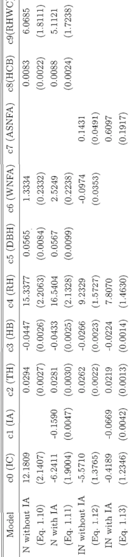
The diameter model appears as the most complex since many covariates were statis­ ticaUy significant : several height measurements (branch height, tree total height, and relative height), and whorl (or annual shoot) number from apex. DBH, crown height and relative height within crown are only significant in the model for nodal branches and annual shoot number from apex only significant for internodal branches. AU of them have a positive coefficient (Table 1.12) with the exception of height to branch, whorl

Model N without lA (Eq. 1.10) N with lA (Eq. 1.11) IN without lA (Eq. 1.12) IN with lA (Eq. 1.13) cO (IC) 12.1809 (2.1407) -6.2411 (1.9004) -5.5710 (1.3765) -0.4189 (1.2346) Tableau 1.12 Coefficients for branch diameter models (with SE) cl (lA) c2 (TH) c3 (HB) c4 (RH) c5 (DBH) c6 (WNFA) 0.0294 -0.0447 15.3377 0.0565 1.3334 (0.0027) (0.0026) (2.2063) (0.0084) (0.2332) -0.1590 0.0281 -0.0433 16.5404 0.0567 2.5249 (0.0047) (0.0030) (0.0025) (2.1328) (0.0099) (0.2238) 0.0262 -0.0266 9.2329 -0.0974 (0.0022) (0.0023) (1.5727) (0.0353) -0.0669 0.0219 -0.0224 7.8070 (0.0042) (0.0013) (0.0014) (1.4630) c7 (ASNFA) 0.1431 _(0.0491) 0.6097 _(0.1917) c8(HCB) 0.0083 (0.0022) 0.0088 (0.0024) c9(RHWC) 6.0685 _(1.8111) 5.1121 _(1.7238) tv <CI

Tableau 1.13 Random effects (SD) for branch diameter models

Model Region Plot Tree AnnualShoot Residual

Model (ar ) (arp ) (arpd (arpta) (érpta)

N without lA (Eq. 1.10) 1.7102 0.5410 1.2558 2.1495 5.8001 N with lA (Eq. 1.11) 0.3794 0.7424 1.6277 2.2717 5.1631 IN without lA (Eq. 1.12) 0.3643 0.1286 0.9272 1.5853 3.8575 IN with lA (Eq. 1.13) 0.0015 0.3117 0.9659 1.6305 3.7157

Tableau 1.14 Prediction errors for branch diameter models

Model AIC E lEI E 2

N without lA (Eq. 1.10) 34188.51 0.0000 4.1023 30.3733 N with lA (Eq. 1.11) 33187.17 0.0000 3.5916 23.4845 IN without lA (Eq. 1.12) 22618.01 0.0000 2.5098 13.3751 IN with lA (Eq. 1.13) 22377.41 0.0000 2.4282 12.3067

number from aeex for the model for internodal branches, and insertion angle. When insertion angle was added, it was the most significant covariate, and improved both mo­ dels as indicated by the AIC (Table 1.14). For the internodal branch diameter, the whorl number from apex became non-significant. The inclusion of insertion angle also caused some minor changes of coefficient values without sign change. Random effects account for a lower proportion explanation of variability than the insertion angle model, with high residuals, followed by annual shoot level, tree level, region, and plot-Ievel random effects (Table 1.13). Despite the complexity of models for diameter, the absolute mean erroris rather high with lEI ranging from 2.4 to 4.1 mm (Table 1.14).

1.5

DiscussiOI

There is a certain level of organization in the way branches are distributed along the annual shoot. In pines in general, and jack pine specifically, they agglomerate in whorls. As the annual shoot elongates, internodal buds are formed until the end of the growing season is marked by the formation of the nodal whor!. This organization brings intrin­

31

sic diflerences in .their growth behavior, which can be observed in differing number of branches formed each year, insertion angle and diameter. Recent studies showed the importance of branch type (nodal versus internodal) in modeling crown development (Achim et al., 2006; Weiskittel et al., 2007). In jack pine, there are on average more nodal branches than internodal branches per annual shoot. Insertion angle is only a lit­ tle more acute for nodal branches, but they grow faster and live longer than internodal branches. Although branch dynamics were not studied here, it can be assumed that the same processes as that of Sitka spruce are at work (Achim et al., 2006) : the larger nodal branches tend to shade the internodal branches, slowing the internodal branch growth and reducing their survival probabilities.

Annual shoot length is without a doubt the best explanatory variable of the number of nodal branches. It seems a good proxy for the environmental conditions needed for bud burst and branch growth initiation. The mean number of nodal branches appears to be age invariant, and varies slightly with the annual shoot length. These results follow previously published data. The number of nodal branches were found to be proportional to annual shoot length for Norway spruce (Colin et al., 1993; Kantola et al., 2007; Hein et al., 2007) and Scots pi ne (Makela et al., 1997; Makinen et Colin, 1999; lVIiikela et J\!Iakinen, 2003). Cardinal direction might play a role as branches were more numerous on the north side as found by Achim et al. (2006). However. cardinal direction was only available for a subsample of our trees, such that its effect on any branch characteristic could not be studied in depth.

The best model predicting the number of internodal branches includes the number of internodal whorls. Preliminary work shows that the number of internodal whorls is proportional to shoot length and inversely proportional to tree age. In summary, for trees with the same number of internodal whorls, stems with better height growth produced more internodal branches. Dominant trees are thus better prepared to insure their apical dominance in case of top damage. Achim et al. (2006) showed for Sitka spruce that the number of internodal branches per annual shoot was higher than that of nodal branches. However this branch type was also characterized by faster self-pruning,

leading to a decreasing number of them at live crown base. In the model of Weiskittel et al. (2007) there were also more internodal branches compared to nodal branches, but as the tree aged, less of them formed. These results are similar to those presented here, where the number of internodal branches depends on the number of internodal whorls that is proportional to annual shoot length, which in turn decreases rapidly when the tree is older than 10-15 years. A trend towards a rapid decrease in internodal branches near live crown base was observed but variables such as RHWC was not significant in our mode!. Self-pruning was minimal close to live crown base even in stands where thinning was performed.

Miikinen et Colin (1998) showed that the branch insertion angle mainly depends on branch age. Our models al! suggest that branch age is the main driver of insertion angle for jack pine. Insertion angle vertical profile of jack pine is also similar to what was observed in other studies (Miikinen et Colin, 1998; Meredieu et al., 1998). This profile is characterized by a rapid increase of insertion angle in the upper part of the crown foHowed by slow~r trend towards tree base. As with jack pine Roeh et Maguire. ~1997) observed that Douglas-fil' bran ch insertion angle rarely exceeds right angle. Branch insertion angle is dictated by two main opposed forces : gravity and counteracting reaction wood formation. As the branch increases in size and weight, it inevitably bends down (Brown, 1971), independently of bran ch type. On the basis of the insertion models where branch diameter is not included, internodal branches present higher insertion angles that change at higher rate with branch age, when compared

ta

the nodal branches. Nodal branches stay longer closer to stem. When branch diameter increases, especially in vigorous trees, it can compensate by removing foliage in the inner crown thus reducing branch weight and preventing ben ding down (Xu et Harrington, 1998). This hypothesis can however not be tested with our jack pine data. It coulù explain how nodal branches can stay alive longer without producing noticeable radial increment. However in order to better understand the effect of branch inclination on radial growth we must use branch curve function parameters instead of insertion angle. Branches can also prolong life by reaching light by bending the branch tip upwards (Wilson, 2000).

In

al! of the insertion

33

angle models, the variances of the random effects and the residuaJs are high. In other words, there is a large variation around the trends predicted by the models.

The branch diameter models are the most complex with the highest number of inde­ pendent variables. Branch position (e.g. height of branch, relative height, whorl and/or shoot number) has a predominant effect on branch diameter. The quantity of light a branch receives inevitably affects its capacity to grow throughout its life. With a snapshot view of branch diameter, it is hard to understand the dynamics of shading and competition between branches and neighboring trees. Nevertheless, it was expected that competition would have a direct effect on branch diameter. To this end, a few au­ thors succeeded in including distance-dependant competitive indices to predict branch diameter (e.g. Makinen et Colin, 1998; Umeki et Kikuzawa, 2000). Competition indices were not found to improve branch characteristics models. Competition effects are felt more in the lower crown (Miikinen, 1999a) and branches at that position might not be numerous enough in our dataset to make variables like stand density emerge as a statis­ tically significant independent variable. On the other hand, Colin et al. (1993) suggested that branch diameter is determined by factors that are linked to growth conditions such as stand history. Tree size variables s1.1ch as DBH and total height can be considered as good indicators of past stand development. Tree size might then be sufficient to account for the past growth conditions and ultimately for the variability of branch diameters, as asserted by Miikinen et Colin (1998). Tree size (total height and DBH) was actually important in our model, leading to the fact that dominant trees have larger branches. For Scots pine, branch growth variability can be partly explained by heritability (Haa­ panen et aL, 1997). It could also be the case for jack pine. Makinen (1999a) showed that branches have the highest growth rates in their first years. The same can be de­ duced from our models, where mean annual branch growth (branch diameter/branch age) follows an inverse exponential function with branch age. Although the data was not sufficient to verify it, cardinal direction may also play a significant role, where sou­ thern branches are bigger due to differential light interception (Achim et aL, 2006). On top of that Rouvinen et Kuuluvainen (1997) suggested that the crown asymmetry