To cite this version :
De León Almaraz, Sofía
and Azzaro-Pantel, Catherine
and Montastruc,
Ludovic
and Pibouleau, Luc
and Baez Senties, Oscar Assessment of mono
and multi-objective optimization to design a hydrogen supply chain (2013)
International Journal of Hydrogen Energy, vol. 88. n° (33). pp. 14121-14145.
ISSN 0360-3199
Open Archive TOULOUSE Archive Ouverte (OATAO)
OATAO is an open access repository that collects the work of some Toulouse researchers
and makes it freely available over the web where possible.
This is an author’s version published in :
http://oatao.univ-toulouse.fr/9722
Official URL :
https://dx.doi.org/10.1016/j.ijhydene.2013.07.059
Any correspondence concerning this service should be sent to the repository administrator :
[email protected]
Assessment of mono and multi-objective
optimization to design a hydrogen supply chain
Sofı´a De-Leo´n Almaraz
a, Catherine Azzaro-Pantel
a,*
,
Ludovic Montastruc
a, Luc Pibouleau
a, Oscar Baez Senties
baUniversite´ de Toulouse, Laboratoire de Ge´nie Chimique, U.M.R. 5503 CNRS/INP/UPS, 4 alle´e Emile Monso, 31432 Toulouse Cedex 4, France
bInstituto Tecnolo´gico de La Paz, Boulevard Forjadores de Baja California Sur No. 4720 Apdo. Postal 43-B, C.P. 23080 La Paz, B.C.S., Mexico
a r t i c l e
i n f o
Keywords:
Multi-objective optimization Hydrogen supply chain MILP 3-Constraint Lexicographic optimization M-TOPSIS
a b s t r a c t
3This work considers the potential future use of hydrogen in fuel cell electrical vehicles to face problems such as global warming, air pollution, energy security and competitiveness. The lack of current infrastructure has been identified as one of the main barriers to develop the hydrogen economy. This work is focused on the design of a hydrogen supply chain through mixed integer linear programming used to find the best solutions for a multi-objective optimization problem in which three multi-objectives are involved, i.e., cost, global warming potential and safety risk. This problem is solved by implementing an -constraint method. The solution consists of a Pareto front, corresponding to different design strate-gies in the associated variable space. Multiple choice decision making is then recom-mended to find the best solution through an M-TOPSIS analysis. The model is applied to the Great Britain case study previously treated in the dedicated literature. Mono and multicriteria optimizations exhibit some differences concerning the degree of centraliza-tion of the network and the seleccentraliza-tion of the produccentraliza-tion technology type.
1.
Introduction
Transportation as an economic activity plays a crucial role in the world. Current transport fuels are mainly obtained from oil, considered as a non-renewable fossil fuel, from which gasoline and diesel are produced. The main advantages of
producing these fuels are related to existing infrastructure, know-how and experience as well as a huge demand allowing efficiency improvement. Yet, prices in fossil fuel vary in each country and the scarcity of oil reserves constitutes a main concern that may lead to an important increase in the fuel prices. Vehicle industry is trying to improve fuel efficiency and
Abbreviations: CCS, carbon capture and storage; CCF, capital charge factor; FCC, facility capital cost; FCEV, fuel cell electric vehicles;
FOC, facility operating cost; GB, Great Britain; GWP, global warming potential; HSC, hydrogen supply chain; ICE, internal combustion engine; LCA, life cycle assessment; LH2, liquid hydrogen; MCDM, multiple choice decision making; MILP, mixed-integer linear
pro-gramming; NTU, number of transport units; PCA, principal component analysis; SCM, supply chain management; SMR, steam methane reforming; TCC, transportation capital cost; TDC, total daily cost; TOC, transportation operating cost; TOPSIS, Technique for Order Preference by Similarity to Ideal Situation.
* Corresponding author. Tel.: þ33 34 32 36 56; fax: þ33 34 32 37 00. E-mail address:[email protected](C. Azzaro-Pantel).
Please cite this article in press as: De-Leo´n Almaraz S, et al., Assessment of mono and multi-objective optimization to design a 0360-3199/$ e see front matter Copyright ª 2013, Hydrogen Energy Publications, LLC. Published by Elsevier Ltd. All rights reserved.
to decrease pollution since CO2tail emissions are responsible
for cardiovascular and respiratory diseases as well as for environmental damages such as those impacting construc-tion materials and other surfaces and also those related to affectation in photosynthesis process and smog. To address the threat of climate change, it is necessary to change and to charge a price for carbon emissions. Besides, governments have to do much more, taking actions to support innovation and diffusion of new, low-carbon technologies [1]. In that context, gasoline and diesel production processes have then been reviewed to be less environmental damaging. The transport sector will probably witness a much more diversi-fied portfolio of fuels in the future, with the share of electric mobility in its broadest sense, i.e. electric-drive vehicles powered by a fuel cell, battery, or a hybrid drive train, ex-pected to increase markedly[2]. Future technologies for in-ternal combustion engine (ICE), hybrid electric cars (battery electric cars or plug-in hybrid electric vehicles) and fuel cell electric vehicles (FCEV) are being developed. The use of different fuels constitutes promising alternatives such as biodiesel, methanol, ethanol, methane, liquefied petroleum gas and hydrogen (H2). Hydrogen which is the most abundant
element in the universe and found in compounds of water and hydrocarbons can be extracted to be used as an energy carrier. The projection of hydrogen use in the vehicular system in fuel cells forces to study some elements of the infrastructure that are not yet well developed or established (i.e. storage, trans-portation and refuelling stations). The study of the so-called hydrogen supply chain (HSC) can help to find different pos-sibilities in the strategic and tactical planning phases for the definition of the H2infrastructure. The originality of this study
is to take into account sustainable development concepts in early stages of the HSC design. For this purpose, three criteria such as economic, social and environmental impacts are optimized at the same time. The remainder of this paper is organized as follows: the next section presents the advantages and obstacles that may be encountered with the HSC. Then, Section3is devoted to a brief review of investigation on HSC. The methodology and objectives of this work are presented in Section4where the general elements of the HSC are shown and the mathematical model followed by the definition of a case study in Section5, results and discussion of mono and multi-objective optimizations are presented in the last sec-tion. Finally, conclusions and perspectives are given.
2.
General context
Currently, most of the hydrogen is produced in petroleum refineries or in the chemical industry and the most common uses of H2are to upgrade fossil fuels and to produce ammonia;
it is then usually consumed onsite. Specifically, only about 5% of hydrogen is considered as “marketable” and delivered elsewhere as a liquid or gas by truck or pipeline[3]. Another use of hydrogen is the storage for electricity from intermittent renewable energies, such as wind and photovoltaic energy. When hydrogen is to become a fully-fledged energy carrier, this also implies the use of hydrogen in the residential and commercial sector [4]. Another interesting application of hydrogen and fuel cells is the power supply of portable or
remote grid consumers like notebooks or telecommunication devices[5].
Hydrogen offers interesting advantages over competitors; first of all it can be obtained from many energy sources (such as water, biomass, coal, natural gas) and production pro-cesses. Fossil fuel sources are the most used nowadays but the implementation of carbon capture and storage (CCS) to steam methane reforming and gasification processes is to be devel-oped. Besides, water electrolysis seems to be the cleaner op-tion when electricity is obtained via renewable energies. In the transport sector well to wheel efficiency of hydrogen as compared to gasoline is higher (about 22e33% vs. 15%)[6]. H2
has also several potential energy uses (heating homes and offices, to stock renewable electricity, portable applications). Another potential benefit from using hydrogen as trans-portation fuel can be found in the form of noise reduction1in
fuel cells.
Reduction in air pollution is also offered by electric cars but several obstacles of use of such vehicles exist such as like the time of the battery recharge, the lack of recharging infrastruc-ture, the high cost associated with the involved lithium battery and perhaps above all a short driving range as compared to ICE or FCEV. Fuel cell technology is well developed and has been rapidly improved in efficiency offering zero emissions at the consumption side. For all these reasons, H2seems to be a good
candidate as an alternative to the current fossil fuel system because it can help to treat problems like global warming, air pollution, energy security and competitiveness.
However, H2faces some obstacles that need to be
over-come before being considered as a viable option. The first problem is the lack of infrastructure[8e11], that represents an investment to install a certain capacity large-scale to produce, store and supply hydrogen through a type of technology while at the same time, the lack of demand estimations or pro-jections makes difficult to estimate the required investment. Consequently this interconnected problem blocks the FCEV penetration to the market. The establishment of a new hydrogen infrastructure for fuel cell vehicles is difficult because no smart transition from gasoline or diesel to hydrogen can be expected due to the lack of bivalent operation modes for such vehicles [5]. In this sense, transition would take years. Timing of the investment over the next 10e30 years will also be critical [8]. Most of studies predict an important market penetration of hydrogen in 2050. For Ball and Wietschel [2], hydrogen production and infrastructure costs are not an economic barrier at today’s prices of con-ventional energy carriers. The critical element is the cost of development of the fuel cell propulsion system, the forecasts being a major source of uncertainty in this case. It is expected that it will take several decades for the build-up of a hydrogen infrastructure and for hydrogen to make a significant contri-bution to the fuel mix.
Moreover, in some countries, safety norms are focused in the production of H2to be used only in chemical processes
1This is achieved since the car is powered by an electric motor
and thus does not have any of the vibration or exhaust noise created by a typical internal combustion engine vehicle. Some of the effects caused by noise pollution can include hearing loss, cardiovascular problems, and inherent unpleasantness[7]. Please cite this article in press as: De-Leo´n Almaraz S, et al., Assessment of mono and multi-objective optimization to design a
with minor transportation and low storage volume. The risk of hydrogen must be considered relative to the common fuels such as gasoline, propane or natural gas; some of H2
proper-ties make it potentially less hazardous, while other charac-teristics could theoretically make it more dangerous in given situations [12]. New technologies could be developed or improved to optimize the HSC, then, security norms should be reviewed and implemented in the whole system for using H2
in vehicles. Comparison between different technology alter-natives in the strategic phase is mandatory.
The lack of social or political interest to promote this type of vehicles is another problem; the governments represent an essential part in building the HSC. Environmental regulations and reduction in taxes for the FCEV could help in the intro-duction phase. Lack of complete scenarios could affect in a bad decision or a disoriented start up in the investment. Without precise assessment, this could represent losses in the total system or at a national project scale.
To study the whole network, tools like supply chain man-agement (SCM) could be applied. Let us recall that supply chain management involves a set of approaches utilized to efficiently integrate suppliers, manufacturers, warehouses, and stores, so that merchandise is produced and distributed at the right quantities, to the right locations, and at the right time, in order to minimize system wide cost while satisfying service level requirements[13]. The focus in SCM can broadly be divided into three main categories, that are design, plan-ningescheduling and control (real-time management); supply chain models can either be formulated with mathematical programming or with simulation oriented approaches while their application depends on the task in hand. The aim of this paper is to study a general HSC using mathematical pro-gramming to design an optimal network so that optimal strategies could be proposed to help decision making.
3.
Literature review
The hydrogen supply chain has been studied from different perspectives; first, geographical approaches are devoted to locate the infrastructure elements in a specified area. Second, optimization methodologies are focused on the search for optimal configuration based on a specific objective; third, another approach to design the HSC networks is simulation. A classification of the main studies is presented here to illus-trate the current methodologies and case studies:
Some examples of geographical approaches include the study of Ball et al.[14]who developed the MOREHyS (Model for Optimization of Regional Hydrogen Supply) approach of the energy system with the integration of geographical aspects in the analysis by the GIS2-based method for Germany.
Johnson et al.[16] used also GIS for modelling regional hydrogen infrastructure deployment using detailed spatial
data and applied the methodology to a case study of a po-tential coal-based hydrogen transportation system in Ohio with CCS. The objective is to optimize hydrogen infrastructure design for the entire state.
Besides, mixed-integer linear programming (MILP) ap-proaches have been widely used for designing the HSC, Almansoori and Shah[17], have clearly introduced a general model that determines the optimal design of a network (pro-duction, transportation and storage) for vehicle use where the network is demand-driven. The model was applied to a Great Britain case study. Later, the same authors extended the model in 2009 [18], to consider the availability of energy sources and their logistics, as well as the variation of hydrogen demand over a long-term planning horizon leading to phased infrastructure development as well as the possibility of selecting different scales of production and storage technol-ogies. Other works[19]take into account demand uncertainty arising from long-term variation in hydrogen demand using a scenario-based approach: the model adds another echelon including fuelling stations and local distribution of hydrogen minimizing the total daily cost.
Hugo et al.[8]developed an optimization-based formula-tion that investigates different hydrogen pathways in Ger-many. The model identifies the optimal infrastructure in terms of both investment and environmental criteria for many alternatives of H2configurations. This model has been
extended and considered as a basis for other works such as Li et al.[11]for the case study in China. At the same time in Iran, a model for investigation of optimal hydrogen pathway and evaluation of environmental impacts of hydrogen supply system was examined by Qadrdan et al.[6]. Another study also considered hydrogen from water, using electricity from hydro and geothermal power in Iceland for exportation[20].
Several perspectives of the HSC have been integrated in Kim et al.[10]models as deterministic vs. stochastic approach to consider demand uncertainty in the new model. The model they proposed determines a configuration that is the best for a given set of demand scenarios with known probabilities. The stochastic programming technique used is based on a two-stage stochastic linear programming approach with fixed recourse, also known as scenario analysis. Later, a strategic design of hydrogen infrastructure was developed to consider cost and safety using multi-objective optimization where the relative risk of hydrogen activities is determined by risk rat-ings calculated based on a risk index method[21].
Guille´n Gosa´lbez et al.[3]proposed a bi-criterion formula-tion that considers simultaneously the total cost and life cycle impact of the hydrogen infrastructure and to develop an effi-cient solution method that overcomes the numerical diffi-culties associated with the resulting large scale MILP. Sabio et al.[22]also developed an approach, which allows control-ling the variation of the economic performance of the hydrogen network in the space of uncertain parameters examined the case study of Spain.
More recently, Murthy Konda et al. [9] considered the technological diversity of the H2supply pathways together
with the spatialetemporal characteristics to optimize a large-scale HSC. They calculate the transportation costs based on Refs.[17]and[18]approaches. The original models are modi-fied (e.g., inclusion of existing plants, capacity expansion and
2GIS: Geographical Information System. It is a package that can
be usefully integrated with a modelling system for supply chain management. The typical GIS contains an extensive database of geographical census information plus graphical capabilities of displaying maps with overlays pertaining to the company’s sup-ply chain activities[15].
pipeline features) and analysis is extended to incorporate the computation of delivered cost of H2, well-to-tank emission
and energy efficiency analyses. In the work of Haeseldonckx and D’haeseleer [4], the objective is not only to find the optimal set of activated hydrogen production plants but also to implement a hydrogen infrastructure optimization algo-rithm that has to decide which hydrogen-production plants will be invested in and which plants will not. Finally, Sabio et al.[23]take into account eight environmental indicators in a two-step method based on a combination of MILP multi-objective optimization with a post-optimal analysis by prin-cipal component analysis (PCA) to detect and omit redundant environmental indicators.
It can be highlighted that several mono-objective optimi-zation approaches have been developed or extended as in Refs. [6,8,10,14,17e19,24]. In these studies the cost is the objective to be minimized. Multi-objective optimization studies are relatively scarce and criteria to be analyzed are based on economic and environmental performances; some examples are presented in Refs.[3,8,11,23]: minimizing the expected total discounted cost and the associated financial risk[22]and minimizing the total cost of the network and the total relative risk of the network[21].
These works are limited to a bi-criteria assessment, generally based either cost-environment or cost-safety. This is not enough when sustainable development must be taken into account in the strategic stage of any new project, when social, economic and environmental impacts are inter-connected: their balance would result in the efficiency of the system. The originality of this study is to consider sustainable development in the HSC design when three criteria such as economic, social and environmental impacts are optimized at the same time.
4.
Methodology
In this section, the main principles of the proposed method-ology are presented. Firstly, the problem statement, assump-tions and objectives are defined with the associated decision variables. The HSC is then presented to establish the general structure of the network. The problem dimension is examined to compare mono and multi-criteria approaches. Finally, the resolution strategy phases are also developed.
4.1. Problem statement
As aforementioned, current designs of the HSC reviewed in the dedicated literature are generally based to a multi-objective strategy with two criteria, either cost-environment or cost-safety. A three-criteria optimization model is pro-posed here considering the interconnection of social, eco-nomic and environmental impacts. Their relationship will result in the global balance of the system.
4.1.1. Objective
This work will be focused in the design of a three-echelon HSC (production, storage and transportation), considering the minimum cost, the lower environmental impact and the lower safety risk. The model will be tested in a relevant case
study (Great Britain) and results for mono-objective optimi-zations will be compared with the multi-objective solution.
4.1.2. Given data
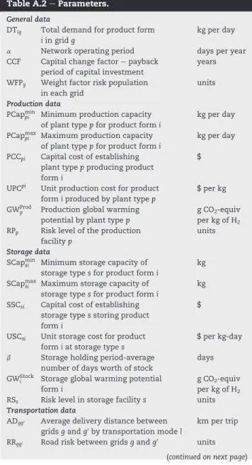
The given data involve hydrogen demand data (each grid has its own deterministic demand), techno-economic, environ-mental and risk data of the components in the HSC (they are presented in detail inAppendix A, Table A.2).
4.1.3. Design decisions
Design decisions are based on the number, type, capacity, and location of production and storage facilities. More precisely, they involve the number and type of transport units required as well as the flow rate of hydrogen between locations. Cities or grids are also considered.
4.1.4. Operational decisions
Operational decisions concern the total production rate of hydrogen in each grid, the total average inventory in each grid, the demand covered by imported hydrogen and the H2
de-mand covered by local production.
4.1.5. Assumptions
" A deterministic demand of hydrogen for the transportation system (particular-light cars and buses) is considered. " A monoperiod problem is assumed.
" Relative risk of production plant, storage facilities and transportation modes are assumed not to change under the various demand scenarios.
" The model is assumed to be demand driven.
4.2. Formulation of the HSC
4.2.1. General structure of the HSC
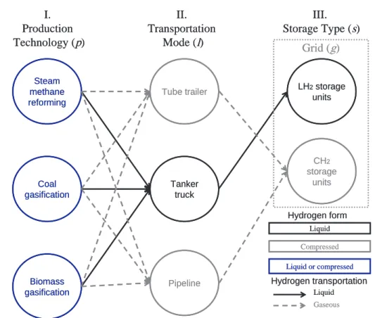
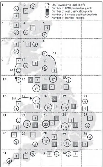
In this formulation, hydrogen can be delivered in specific physical form i, such as liquid or/and gaseous, produced in a plant type with different production technologies p (i.e. steam methane reforming (SMR), biomass or coal gasification); distributed by a specific type of transportation modes l going from the location g to g0referred as grid squares; such that g0is
different than g; these grid squares are obtained by dividing the total area of the country or region into n grid squares of equal size, a general HSC is shown inFig. 1. This supply chain is demand driven and it is a reverse logic network because we assume there are no flows from the market to the facilities or suppliers.
4.2.2. Supply chain decision database
Several data are necessary to design the HSC as the base investment and operational costs for a given facility that will be used for extrapolation purpose, the throughput associ-ated with a given technology, the quantities of input and output products associated with unit operations of the transformation types, etc. The whole list is presented in
Appendix B.
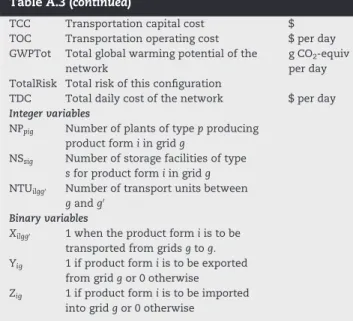
4.2.3. Model variables
The definition of continuous, integer and binary variables is necessary for the mathematical formulation of the HSC Please cite this article in press as: De-Leo´n Almaraz S, et al., Assessment of mono and multi-objective optimization to design a
(detailed classification is shown inAppendix A, Table A.3). The problem is then captured in a mixed-integer linear program-ming (MILP) framework. All continuous and integer variables must be non-negative. Output data will include optimal lo-cations and capacities of new facilities, levels for trans-formation and process activities at each facility, outbound flows of finished products from production facilities to mar-kets, etc.
4.3. Mathematical model
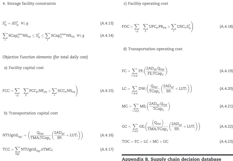
This work is inspired from the previous model of Almansoori and Shah[17]. For reasons of brevity, not all the equations are presented here but mass balance, production, transportation and storage constraints can be found inAppendix A.4where different constraints features (i.e. equality or inequality, binding and nonbinding) are easily appreciated.
One modification was made to the original model[17]. It consists in the way to calculate the number of transport units (NTU) because it did not take an integer value. Values of transportation capital cost (TCC) and transportation operating cost (TOC) were lower than the real cost considering integer values. Eqs. (1) and (2) were added to the model and Eq.
(A.4.16),3was modified inAppendix A.4to allow rounding the
NTU value throughEq. (3).
Vilgg0$0 ci; l; g; g0 (1)
Vilgg0%1 & Xilgg0 ci; l; g; g0 (2)
where Vilgg0is a continuous variable with values between 0 and
1 related to the binary value of Xilgg0which takes the value of 1
when the product form i is to be transported from grids g to g0.
Then NTUilgg0depends significantly on the average distance
travelled between different grids ðADgg0Þ, the capacity of a
transport container ðTCapilÞ, the flow rate of products between various grids ðQilgg0Þ, the transportation mode availability
ðTMAlÞ, the average speed (SPl), and loading/unloading time
(LUTl). Finally, the Vilgg0is added and an integer value is found.
NTUilgg0¼ ! Qilgg0 TMAlTCapil !2AD gg0 SPl þLUTl "" þVilgg0 (3) 4.3.1. Cost objective
The total daily cost (TDC) of the network is determined in the same way as in the linear model of Almansoori and Shah[17]. Some comments are given below.
1. Total capital cost e including facilities and transportation modes ($ per day).
Capital costs for a plant p or a storage facility s are defined as parameters. Then, the costs correspond to the product of the number of new plants and of the number storage units (integer variables) to be installed. Similarly, the trans-portation capital cost is calculated by multiplying the cost of transport modes by the number of new transport units (integer variable). Both facility and transportation costs are added and divided by the product of the capital change factor (a value of three years is considered as in Ref.[17]and of the network operating period (assumed to be 365 days per year)).
I.
Production
Technology (
p
)
II.
Transportation
Mode (
l
)
III.
Storage Type (
s
)
Coal gasification Biomass gasification Tanker truck Steam methane reforming Tube trailer Pipeline LH2storage units CH2 storage units Liquid Compressed Liquid or compressed Hydrogen form Hydrogen transportation Liquid GaseousGrid (
g
)
Fig. 1 e A general hydrogen supply chain.
3Replaced byEq. (3)of Section4.3.
2. Facility operating cost ($ per day).
This value is constituted by the addition of two terms. The former term corresponds to the product of the unit produc-tion cost ($ per kg H2) and of the average production rate
given in kg per day (continuous variable). The latter term is the product of the unit storage cost ($ per kg H2per day) and
of the average storage rate in kg H2(continuous variable).
3. Transportation operating cost ($ per day).
It is based on the determination of four costs related to transport units:
"Fuel cost ($ per day) corresponds to the product of fuel price ($ per L) and of the daily fuel usage (L per day); this function takes into account data such as the average distance to be driven, fuel economy, transportation ca-pacity as well as the flow rate of products between various grids (kg per day, as a continuous variable). "Labour cost ($ per day) which is obtained by the product of
the driver wage ($ per hour) and of the total labour time (hours per day) constituted by the continuous variable of the flow rate of products between various grids (kg per day) and given data such as the transportation capacity (kg per trip), the round trip distance (km), the average speed and the load and unload time of hydrogen (hours). "Maintenance cost ($ per day) is defined as the product of maintenance expenses ($ per km) and of the total daily distance driven. It involves the product of the round trip distance (km) and of the continuous variable of the flow rate of products between various grids (kg per day), then divided by the transportation capacity (kg per trip). "General cost ($ per day) consists of transportation
insur-ance, license and registration, and outstanding finances. It depends on the integer variable of number of transport units.
The TDC represents the cost expressed in $ per day of the entire HSC where FCC is the facility capital cost ($), TCC is the transportation capital cost ($), a is the network operating period (days per year) related to the capital charge factor (CCF, in years). Then, the facility operating cost (FOC, $ per day) and the transportation operating cost (TOC, $ per day) are also associated inEq. (4).
TDC ¼
!FCC þ TCC
a$CCF "
þFOC þ TOC (4)
The addition of new constraints to find global warming potential and safety risks values are necessary to imple-ment the proposed multi-objective approach. The definition of the additional objective functions considered is pre-sented below.
4.3.2. Global warming potential objective
The global warming potential (GWP) is an indicator of the overall effect of the process related to the heat radiation ab-sorption of the atmosphere due to emissions of greenhouse gases (CO2-equiv) of the network[25]. The total daily
produc-tion GWP (PGWP, in g CO2-equiv per day) is associated with the
production rate of product type i produced by each plant of type p in grid g (PRpig, in kg per day) and the total daily GWP in the production facility type p (GWprodi , in g CO2-equiv per kg):
PGWP ¼X pig $ PRpigGWprodi % (5) The total daily storage GWP (SGWP, in g CO2-equiv per day)
is given byEq. (6)where the PRpigis related to the total daily
GWP for the storage technology (GWstock
i , in g CO2-equiv per kg): SGWP ¼X pig $ PRpigGWstocki % (6) The total daily transport GWP (TGWP, in g CO2-equiv per
day) is determined as follows:
TGWP ¼X ilgg0 !2AD lgg0$Qilgg0 TCapil " GWTrans i $Wl (7)
where the average delivery distance between g and g0 by
transportation mode l (km trip*1) is multiplied by the flow
rate of product form i transported by the mode l between g and g0 and divided by the transportation capacity for
product form i (kg trip*1). These three terms allow the
computation of the number of km per day that must be run to cover the demand taking into account the round trip. Finally those terms are related to the global warming potential (GWTrans
i , in g CO2-equiv per tonne-km)
associ-ated to the transportation mode l and its weight (Wl, in
tons).
Eqs. (5)e(7) enable the calculation of the total GWP (GWPTot, in g CO2-equiv per day) as indicated by:
GWPTot ¼ PGWP þ SGWP þ TGWP (8)
4.3.3. Safety objective
Kim and Moon[21,26]developed expressions to evaluate the total risk of production and storage facilities (TPRisk and TSRisk respectively) as well as the total transport risk (TTRisk) where the relative risk of hydrogen activities is determined by risk ratings calculated based on a risk index method. The TPRisk is calculated as follows:
TPRisk ¼X
pig
&NPpig$RPp$WFPg
'
(9) where NPpig is the number of plants of type p producing
product form i in grid g, RPpis the risk level of the production
facility p and WFPg is the population weight factor in g in
which a production or storage facility is located. The TSRisk is related to the number of storage facilities of type s for prod-ucts form i in grid g ðNSsigÞ, the risk level in storage facility s
ðRSsÞand the WFPgas indicated by:
TSRisk ¼X
sig
&NSsig$RSs$WFPg
'
(10) The TTRisk is associated with the number of transport units from g to g0 ðNTU
ilgg0Þin each grid, the safety risk level of
transportation mode l ðRTlÞand the road risk between grids g
and g0ðRR
gg0Þ. The equation adopted in what follows is:
TTRisk ¼X
ilgg0
NTUilgg0$RTlRRgg0 (11)
By combiningEqs. (9), (10) and (11), the total relative risk (TR) is given by:
TR ¼ TPRisk þ TSRisk þ TTRisk (12)
4.4. Problem dimension
The mono-objective problem dimension treated in Ref.[17]
was compared with the multi-objective approach considered in our work to analyze the statistics and main differences (see
Table 1). The problem was solved minimizing TDC for both cases but the new constraints presented in Sections4.3.2 and 4.3.3 were added for the multi-objective case. Then, the number of constraints was doubled and similar results were observed for the number of integer and continuous variables. The computational time increased by a factor of 37% in the multi-objective case. The model dimension involves 12,464 constraints and 6242 variables (among them, 2516 are integer).
4.5. Solution strategy
In a preliminary phase, each mono-criterion problem was optimized separately to analyse how its optimal values are decreased when making a multi-criteria optimization.
4.5.1. Preliminary phase: mono-objective and lexicographic optimization
The geographical area (country or region) to be studied is selected and divided in grids or sub-regions. The possible configurations of the HSC to be located in that place are defined (such as product physical form, viable production processes, transportation type, etc..). The mathematical model is then formulated within the GAMS 23.9[27] environ-ment and solved using CPLEX. Each independent objective function is to be minimized using a lexicographic optimiza-tion strategy that produces only efficient soluoptimiza-tions when all the objectives are considered.
Mavrotas[28]proposes the use of lexicographic optimiza-tion for every objective funcoptimiza-tion in order to construct the payoff table with only efficient solutions. A simple remedy in order to bypass the difficulty of estimating the nadir values of the objective functions is to define reservation values for the objective functions. The reservation value acts like a lower (or upper for minimization objective functions) bound.
Practically, the lexicographic optimization is performed as follows: an objective function (of higher priority) is first opti-mized, obtaining min TDC ¼ z1*. Then, a second objective function is optimized (total GWP) by adding the constraint TDC ¼ z1* in order to keep the optimal solution of the first opti-mization, in order to obtain min GWP ¼ z2*. Subsequently, the third objective function is optimized by adding the constraints TDC ¼ z1* and GWP ¼ z2* in order to keep the previous optimal solutions and so on until all the objective functions are treated in a more general case involving more objective functions.
4.5.2. Solution phase: multi-objective optimization
The payoff table designed from the application of the lexico-graphic optimization allows defining the solution. In this approach which tries to minimize all objective functions, the optimal values represent the lower bounds (utopia points) of each objective in the feasible space and the nadir points are relative to values corresponding to the upper bounds on the Pareto surface, and not in any feasible space (values worse than the reservation value are not allowed).
The tri-objective optimization problem is solved by imple-menting the 3-constraint method. Once the epsilon points
(in-termediate equidistant grid points) are defined, the objective function TDC has to be minimized. The GWP and TR objective functions are then transformed into inequalities constraints.
The global model can be formulated in a more concise manner as follows:
Minimize {TDC}
The objective of this formulation is to find values of the operational x˛Rn,and strategic y˛Y ¼ {0,1}m, z˛Zþ decision
variables, subject to the set of equality h(x,y) ¼ 0 and inequality constraints g(x,y) % 0. In this model, the contin-uous operational variables concern decisions dedicated to production, storage and transportation rate, whereas the discrete strategic variables capture the investment de-cisions such as the selection of activity types and trans-portation links.
All costs, emissions and risk equations occur as linear functions of the associated decision variables levels. That means the production, storage and transportation costs, GWP Table 1 e Statistics for mono and multi-objective
approaches.
Type of optimization
Mono-objective
Multi-objective
Number of constraints 6197 12,464
Number of integer variables 1326 2516
Number of continuous variables 1369 3726
CPU time (s) 717 987 Optimal gap (%) 0.01% Subject to : hðx; yÞ ¼ 0 gðx; yÞ % 0 x˛Rn;y˛Y ¼ f0; 1gm ;z˛Zþ Risk ¼ 3nðn ¼ 0; 1; 2; .; NÞ Total GWP % 3mðm ¼ 0; 1; 2; :::; MÞ 8 > > > > > > > > < > > > > > > > > : Demand satisfaction Overall mass balance Capacity limitations Distribution network design Site allocation
Cost; environmental and risk correlations Non-negativity constraints 9 > > > > > > > > = > > > > > > > > ;
and safety risk levels are linear values of the associated de-cision variables. The solution consists of a Pareto front composed of solutions that represent different possibilities of supply chain configurations.
4.5.3. Multiple choice decision making (MCDM)
A TOPSIS (Technique for Order Preference by Similarity to Ideal
Situation[29]) analysis is carried out on the Pareto front with the same weighting factor for the cost, safety and environ-mental criteria. Then, a modified synthetic evaluation method (M-TOPSIS)[29,30]is also used since it is particularly efficient to avoid rank reversals (unacceptable changes in the ranks of the alternatives[31]) and to solve the problem on evaluation failure that may occur in the original TOPSIS version.
5.
Case study
A general HSC is presented in Fig. 1, where the hydrogen form could be liquid or gaseous and some transportation modes and storage facilities are available. A case study of Great Britain (GB) treated by Almansoori and Shah[17]has also been analyzed to illustrate the main capabilities of the new proposed model. GB is divided into 34 grid squares of equal size. Three different production processes are evalu-ated: SMR, biomass and coal gasification. Hydrogen has to be liquefied before being stored or distributed. Liquid hydrogen (LH2) is stored in super-insulated spherical tanks then
delivered via tanker trucks. Almansoori and Shah[17] esti-mated the total hydrogen demand in Great Britain as a function of the total number of vehicles, average total dis-tance travelled and vehicle fuel economy (seeAppendix B, Table B.1). The estimated demand is assumed to supply private-and-light goods vehicles and buses at 2002 levels. This is based on the assumption that 100% of the above-mentioned vehicles would be powered by proton exchange membrane fuel cells (13,392 t per day). Four cases will be analyzed (seeTable 2) and compared with those of the base
case [17]. Case 1 consists in the minimization of the total daily cost both with a variant approach to compute NTU and a more recent solver version, CPLEX 12 versus CPLEX 9 as the approach used in Ref.[18]. Case 2 minimizes the total global warming potential (CO2emissions) of the network. Case 3 is
devoted to the minimization of safety risk. Finally, Case 4 concerns the simultaneous optimization of the three-abovementioned criteria.
5.1. Techno-economic data
A large amount of input data is required to solve the problem. All the techno-economic parameters (i.e., minimum and maximum production and storage capacities, average delivery distance between grids and capacity of each transportation mode, etc.) are defined inAppendix B.
5.2. Environmental data
As new constraints are integrated to the model, new data were collected to compute the emission of each activity of the supply chain. It must be emphasized that an exhaustive life cycle assessment (LCA studies the impact and effects of a product from the purchase of the raw material until its utili-zation and elimination. ISO 14040) was not performed. Only CO2 emissions relative to production, storage and
trans-portation were evaluated. Strømman and Hertwich in Ref.[32]
reported that the GWP for the SMR (without CO2capture and
depository) process was of 10,100 g CO2-equiv per kg H2
pro-duced. The same indicator results in 10,540 g CO2-equiv per kg
when hydrogen is produced via coal gasification (underground mined coal) [33]. Biomass gasification leads to 3100 g CO2
-equiv per kg [25]. After liquefaction process, H2 storage in
spherical tanks results in 5251 g CO2-equiv per kg H2according
to the Detailed California Modified GREET pathway in 2009[34]
including manufacture, construction facilities, fuel con-sumption, flare combustion and methane venting. Moreover, an amount of 62 g CO2-equiv per tonne-km is emitted by
tanker truck transportation[35]and the weight of the trans-portation taken into account is 40 t[36].
5.3. Safety data
The evaluation of the safety risk takes as parameters three indicators, i.e., the risk level of each activity, the population weight factor and the adjacency level in transportation links. For the risk level of each activity (H2production-storage
fa-cilities and transportation units), Kim et al. [21] [26] have developed a risk assessment methodology through the hazard identification using the failure modes and effects analysis (FMEA) and the consequence-likelihood analysis to complete the risk evaluation (each hazard is plotted on a frequency vs. consequence matrix (risk binning matrix), that indicates its level of risk as high, moderate, low, or negligible). The risk-binning matrix in Ref. [21] summarizes the individual risk and relative risk level according to its remark raking and is taking into account for our database. All hydrogen activities considered are marked as Levels IIeIV according to harmful-ness for people, the environment and facilities. The accep-tance criterion of these levels is described in Appendix B, Table B.5. A risk level III corresponds to SMR, tanker truck and liquid storage. Values for biomass and coal gasification were not found, then, they were assumed to have the same risk level as SMR.
The population risk weight factors for each grid are clas-sified inTable 3, i.e., when the population of a particular grid is over 2 millions, we assume that this region has a score of 5, from 1 to 2 millions the score is 4 and so on. According to this Table 2 e Different case studies and objectives to be
analyzed. Minimization of Total daily cost Global warming potential Total risk Base case X Case 1 X Case 2 X Case 3 X Case 4 X X X
classification, a higher weighting rate for grids corresponds to a higher population density.
The adjacency level in transportation links was calculated as a function of the crossed grids or those close to the road. If hydrogen is transported through some intermediate grids, the impacts on these regions must be taken into account as indicated in the following equation:
RRgg0¼ X g &RLgþ bg2RLg2þ bg3RLg3þ . þRLg0 ' (13) where subscripts g and g0represent the first and last regions
and g1, g2, ., gnrepresent the intermediate regions through
which hydrogen is transported; bgis the weight factor that
indicates the adjacency level of a region in which the route is located. It takes a rating value between 0.1 and 1.0 ac-cording to the adjacency level. For a transiting grid, the value is 1, for a close region, the value is 0.5, this value is multiplied by the risk level of the grid (RLg, see Table B.6)
classified according to the grid size e by population density (i.e., small ¼ 1, medium ¼ 2 or large ¼ 3). This calculation is detailed in the method proposed by Kim and Moon[26]. Due to the geographical division of the original case study[17], some difficulties were encountered to pre-cisely locate the roads. The following method was then adopted: if hydrogen produced in region 1 is transported to region 33, this transportation arc has to penetrate nine grids ( g1, g4, g7, g10, g13, g17, g23, g28 and g33) and is close to four grids ( g2, g3, g18 and g22); applyingEq. (13), the external effect factor of the transportation arc from region 1 to 33 is 25.5 (seeTable B.6). Appendix B, Table B.4shows the total
relative risk matrix for impact on city transportation be-tween grids. The highest risk line is the hydrogen trans-portation from grid 31 (565) and the lowest risk line concerns hydrogen transportation from grid 17 (335). If decision-makers design the hydrogen supply chain by considering only transportation safety, it is safer to completely avoid transportation from grid 31.
6.
Results and discussion
The different stages of the proposed methodology were developed and applied in the abovementioned case study. In this section, the results and corresponding configurations are analysed and discussed in detail. In a preliminary phase, the three criteria were optimized separately to analyse how their optimal values decrease when making a multicriteria opti-mization. The 3-constraint method is applied and the best
compromise solution is then chosen from the Pareto front via M-TOPSIS.
6.1. Preliminary phase
The preliminary phase allowed finding the payoff table through lexicographic optimization (see Section 4.5). Thus, it is possible to obtain as the solution that minimizes TDC as the one that corresponds to point that is a non-dominated solution also for total GWP and total risk. The optimization runs were performed for cases 1, 2 and 3 where cost, CO2 emissions and safety risk are to be
mini-mized. The results of each independent optimization can be seen in Table 4. The optimization runs were implemented with a Pentium (R) Dual-core CPU [email protected] GHz proces-sor machine.
Following the conventional optimization we first calculate the payoff table by simply calculating the individual optima of the objective functions. The conventional MILP optimizer will produce the payoff table shown inTable 4(a). However, it is almost sure that a conventional MILP optimizer will calculate the solution of the first point and will stop the searching giving this solution as output. In order to avoid this situation, the Table 3 e Relative impact level of grids based on the
population density.
Population level (persons per grid) Grids
Level 1 (under 2.5Eþ05) 2,5,8,9,12,16,20,21,26,34
Level 2 (2.5Eþ05 e5Eþ05) 1,3,4,6,7,15,30,31,32,33 Level 3 (5Eþ05 e1Eþ06) 10,11,17,19,25,27 Level 4 (1Eþ06 e2Eþ06) 13,22
Level 5 (over 2Eþ06) 14,18,23,24,28,29
Table 4 e Comparison between conventional (mono-objective) and lexicographic optimization results. (a) Payoff table obtained by a
conventional MILP optimizer
(b) Payoff table obtained by the lexicographic optimization
Case 1 2 3 1 2 3
Minimize TDC GWP TR TDC GWP TR
Total network cost M($ per day)
64.57 135.92 77.57 64.57 132.05 73.65
Total GWP
(103t CO
2-equiv per day)
205.86 111.85 203.35 205.86 111.85 205.6
Total risk (units) 10,363 6005 5970 10,292 5970 5970
TDC: total daily cost.
GWP: global warming potential. TR: total risk.
lexicographic optimization of the objective functions is per-formed and the results are shown in Table 4(b). It can be highlighted that the optimal solution obtained through con-ventional optimization of TDC (TDC ¼ 64.57 M$ per day, total GWP ¼ 205.86 - 103t CO
2-equiv per day and total risk ¼ 10,363
units) is a dominated solution in the problem due to alterna-tive optima resulted through the lexicographic optimization (TDC ¼ 64.57 M$ per day, total GWP ¼ 205.86 - 103t CO
2-equiv
per day and total risk ¼ 10,292 units); the total risk is decreased by 71 units. The same analysis can be made for the two other objective functions. The bold characters inTable 4(it will be also the case inTables 5and6) are relative to the value of the optimized criterion for the mono-objective optimization and in the case of the lexicographic optimization is related to the first optimized objective (higher priority).
Information concerning the decision variables is presented inTable 5. The values of flow rates between grids, total pro-duction and storage per day in each location can be found in
Appendix C. All the mono-objective cases are analysed in the next section.
6.1.1. Base case and case 1 (minimal TDC)
The results obtained in case 1 are in agreement with the base
case [17]. The minimal number of 28 production plants is obtained with steam methane reforming (SMR) technology dispersed throughout GB territory. Production of LH2via SMR
has also been found in previous works[23,24], with cost as an objective function. The number of storage units is 265 when adopting the same value for demand and with a storage period of 10 days. Case 1 involves 171 tanker trucks to cover the demand between grids which represents a transportation capital cost of 85.5 M$ as compared with 80.2 M$ in Ref.[17]
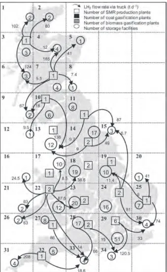
where the number of transport units is not reported. Trans-portation costs (i.e., fuel, labour, maintenance and general costs) are directly influenced by the number of trips, trip distances and number of transport units for each case. Among all the case studies, the higher transportation cost is observed for case 1 when minimizing TDC: less plants are installed but more transport units are required to cover all the national demand, consequently, the transportation operating cost is also higher and the network results in a centralized HSC with the minimal total daily cost for the network of 64.57 M$.
The configurations that can be obtained are presented in
Figs. 2and3and exhibit low differences in the distribution links and liquid hydrogen amounts to be transported between
base case and case 1. The minor variations that can be
observed could be attributed to the solver version. In case 1, less distribution links are found but the amount of LH2
transported keeps the same value. The imported part of de-mand of LH2between grids and the flow rates is listed in Appendix C, Table C.2.
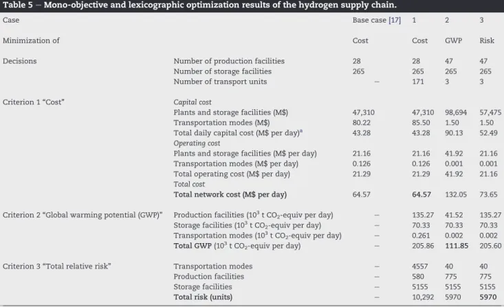
Table 5 e Mono-objective and lexicographic optimization results of the hydrogen supply chain.
Case Base case[17] 1 2 3
Minimization of Cost Cost GWP Risk
Decisions Number of production facilities 28 28 47 47
Number of storage facilities 265 265 265 265
Number of transport units e 171 3 3
Criterion 1 “Cost” Capital cost
Plants and storage facilities (M$) 47,310 47,310 98,694 57,475
Transportation modes (M$) 80.22 85.50 1.50 1.50
Total daily capital cost (M$ per day)a 43.28 43.28 90.13 52.49
Operating cost
Plants and storage facilities (M$ per day) 21.16 21.16 41.92 21.16
Transportation modes (M$ per day) 0.126 0.126 0.001 0.001
Total operating cost (M$ per day) 21.29 21.29 41.92 21.16
Total cost
Total network cost (M$ per day) 64.57 64.57 132.05 73.65
Criterion 2 “Global warming potential (GWP)” Production facilities (103t CO
2-equiv per day) e 135.27 41.52 135.27
Storage facilities (103t CO
2-equiv per day) e 70.33 70.33 70.33
Transportation modes (103t CO
2-equiv per day) e 0.261 0.002 0.002
Total GWP (103t CO
2-equiv per day) e 205.86 111.85 205.60
Criterion 3 “Total relative risk” Transportation modes e 4557 40 40
Production facilities e 580 775 775
Storage facilities e 5155 5155 5155
Total risk (units) e 10,292 5970 5970
a Assuming a capital charge factordpayback period of capital investment of 3 years and the network operating value in 365 days per day. Demand 13 392 360 kg per day.
6.1.2. Case 2 (minimal GWP)
Case 2 is relative to the minimization of the global warming
potential. Minimal total GWP resulted in 111.85 - 103t CO 2
-equiv per day in which the main contribution is given by the liquid storage process (62%), followed by the amount emitted by the production facilities (37%) and a minimal impact of transportation (only three tanker trucks are considered in this network). In the case of storage facilities, the solver does not change the amount of facilities installed since there is only one size of storage tank, so that the optimization is only performed with the number of production facilities and transportation units as significant decision variables. The number of production plants increase considerably (from 28 plants in case 1 to 47 in this case) and all of them are biomass gasification facilities. The kind of technology plays a key role in the CO2 emissions: biomass gasification technology
de-creases GWP but represents also a higher investment affecting the total daily cost of the HSC which is more than two times higher compared to the case 1. Guille´n et al.[3]
also found that the most promising alternative to achieve significant environmental savings consisted in replacing SMR by biomass gasification. InFig. 4, it can be highlighted that only three transportation links are established (from grids 9 to 10, 11 to 8 and from 16 to 17). As mentioned in Guille´n et al.[3], case 2 HSC design results in a decentralized network where almost all the grids are autonomous in LH2
production.
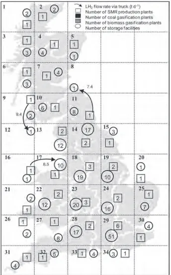
6.1.3. Case 3 (minimal relative risk)
Case 3 minimizes the total relative risk. The optimal
configuration is shown in Fig. 5. Figs. 4 and 5 show simi-larity in the degree of decentralization with only three distribution links and three tanker trucks assigned for the whole supply chain. Less links and transport units are assigned and are related to a higher number of installed production facilities, which is consistent with the results of
cases 1 and 2. Specific features for case 3 can be highlighted
for production units with a total of 47 facilities located in Fig. 3 e Network structure of liquid hydrogen produced via medium-to-large SMR plants, stored in medium-to-large storage facilities, and distributed via tanker trucks for the case 1 (cost minimization).
Fig. 2 e Network structure of liquid hydrogen produced via medium-to-large SMR plants, stored in medium-to-large storage facilities, and distributed via tanker trucks. Cost minimization (Almansoori and Shah, 2006).
all the grids except in grid 8 and 12; even though Kim and Moon [26]found that the installation of plants changed in those grids with less population density, this was not found here (i.e. grid 29 involves a total of 6 production units). The main difference between case 2 and 3 is the production technology which results in 100% of installed SMR plants when risk is minimized.
The total relative risk for this case is of 5970 units and is basically influenced by the storage risk (86%) since storage is scattered in each grid to cover a volume equivalent to 10 days of demand of LH2per grid. Yet, from the results of this case
study, it cannot be deduced that safety risk will be lower if more small storage units are installed since the different storage sizes were not considered. A variation in the number of storage units was not found. The production risk is the second major risk (13%). The transportation relative risk was reduced to find a more safety configuration considering at the same time the links and distance to be run. It must be pointed out that the number of tanker trucks was dramatically
reduced from case 1 to cases 2 and 3 (from 171 to 3 units); in the second case this was made to decrease GWP but in this case the transportation risk represented 44% in case 1 and repre-sents less than 1% for case 3. Through analysis of production plants and the transportation modes, Kim and Moon [21]
determined that changing the type of plant or mode does not offer additional financial benefits or safety guarantees. Yet, in our case, we found that the production technology mix of case 3 represents a financial benefit of 44% as compared to the second case where 100% of biomass gasification plants were installed.
6.2. Multi-objective optimization
From the three independent mono-objective cases, each objective function range can be obtained so that, the
3-constraint method can be applied. From the lexicographic
optimization results ofTable 4(b), the utopia and nadir points of each criterion can be found. The total risk can be divided Fig. 4 e Network structure of liquid hydrogen produced via
medium-to-large biomass gasification plants, stored in medium-to-large storage facilities, and distributed via tanker trucks for the case 2 (CO2minimization).
Fig. 5 e Network structure of liquid hydrogen produced via medium-to-large SMR plants, stored in medium-to-large storage facilities, and distributed via tanker trucks for the case 3 (risk optimization).
into three intervals to make the interpretation easier: low
risk ¼ 5970 corresponding to the best possible obtained, me-dium risk ¼ 8132 (the intermediate value defined by the
ep-silons 3n) and high risk ¼ 10,292 units corresponding to the
nadir point according the payoff table. Similarly, 15 epsilon points were defined for GWP. Then, the objective function TDC has to be minimized while total GWP and total risk are considered as inequality constraints. The solution consists of a Pareto front composed of solutions for supply chain con-figurations (seeFig. 6). The cost of both high and medium risks is similar since these two levels of risks have close impacts of CO2emissions, that is because of the degree of centralization
higher in the high risk network and also with longer route links and with more trips per day. This represents a benefice in TDC compared with the low risk. InFig. 6lines of medium and high risks options are very close, according to this result if the decision maker prefers to decrease the safety risk from high to medium, this decision will not represent a high cost affectation compared to the investment cost that would be necessary to change from high to low risk. The degree of decentralization in the low risk is the main difference and at the same time the impact of the technology type that impacts directly the cost and the GWP (i.e. the capital cost of estab-lishing biomass gasification plant is of M$ 1412 vs. M$ 535 for the SMR technology[17]). Then if the risk level is to be low and to assure to emit less CO2 a higher investment is
necessary.
Five points are plotted (AeE ) in the Pareto front (see
Fig. 6) to give an example of the difference in the degree of decentralization. The point A is the most centralized configuration with 36 distribution links and 171 tanker trucks assigned for the whole supply chain. The flow rate for this configuration can be seen in Table C.1. This solution corresponds to a high risk with low cost with a maximum of CO2emissions. At the same time, the point B is connected by
26 links and 115 tanker trucks, similar results are found for the other solutions of medium risk. Finally, a low degree of centralization is found for solutions with low risk, points CeE require only 3 transport units to distribute less then 1% of the total daily demand of hydrogen, the remaining part is produced on-site.
The 43 possible set solutions in the Pareto front were evaluated via TOPSIS and M-TOPSIS analysis[29,30] carried out with the same weighting factor for the cost, safety and environmental factors (seeAppendix C, Table C.3).
6.2.1. Case 4 (multi-objective optimization)
Based on the data and assumptions, the optimal configuration of the future HSC involves 47 production plants as a mix of production technologies (i.e. 66% for SMR and 34% for biomass gasification) located in a decentralized configuration. This network uses tanker trucks to deliver liquid LH2to storage
fa-cilities. This option involves a TDC of 97.97 M$ per day, a GWPTot of 153.63 - 103t CO
2-equiv per day and a low safety risk.
Fig. 6 e Pareto solutions for the multi-objective model.
Table 6 e Multi-objective optimization results of the hydrogen supply chain.
Case 4
Minimize Cost, GWP and
risk
Decisions Number of production
facilities 47 Number of storage facilities 265 Number of transport units 3
Criterion 1 “Cost” Capital cost
Plants and storage facilities (M$)
71,507 Transportation
modes (M$)
1.50 Total daily capital cost
(M$ per day)a
65.30
Operating cost
Plants and storage facilities (M$ per day)
32.67 Transportation modes (M$ per day)
0.001 Total operating cost
(M$ per day)
32.67
Total cost
Total network cost (M$ per day) 97.97 Criterion 2 “Global warming potential” Production facilities (103t CO
2-equiv per day)
83.30 Storage facilities
(103t CO
2-equiv per day)
70.33 Transportation modes
(103t CO
2-equiv per day)
0.002 Total GWP
(103t CO
2-equiv per day)
153.63
Criterion 3 “Risk” Transportation modes 40
Production facilities 775
Storage facilities 5155
Total risk (units-level) 5970
a Assuming a capital charge factordpayback period of capital in-vestment of 3 years and the network operating value in 365 days per day. Demand 13,392,360 kilos per day.
The results concerning the decision variables for the multi-objective optimization problems are displayed inTable 6and
Fig. 7shows the corresponding configuration. The analysis of the network is quite different from the mono-objective
configuration of Fig. 3. In the base case, it can be observed that long transportation links are installed between grids because such an option is cheaper than building a new pro-duction facility. It must be emphasized that the degree of decentralization increases in the multicriteria solution and is similar in cases 2 and 3.
The change from a centralized to a decentralized supply chain is the main difference observed when the safety risk and the CO2 emissions are taken into account in the
opti-mization phase. The production plants work with less ef-ficiency because they have a maximum capacity of 480 t per day and in some cases they are producing only 10 t per day. Different plant sizes could be studied in a future approach.
Table 7 shows that the best value obtained for TDC in the multi-objective approach (case 4) is higher (an increase by 34% is observed) than for mono-objective case (case 1). Moreover, the CO2 emissions and the risk are improved in case 4 reducing GWP by 34% and the total risk by 72%. The
total GWP decreases by 27% in case 2 as compared with case
4 while the reduction in CO2 emissions implies a higher
cost (35%) while not affecting the risk. Finally, the minimal risk was found in cases 3 and 4 (best results are shown in
Table 4 for the lexicographic optimization) but the other two criteria are different. The TDC increases by 25% in case
4 but the CO2emissions are decreased by 34% as compared
with case 3.
Finally, the unitary cost of hydrogen per case is presented inFig. 8. It must be highlighted that no refuelling station is included in this optimization of the HSC, even though these results could give us an idea about the competitiveness of H2
with fossil fuels. One kilogram of hydrogen is approximately equivalent to one gallon of gasoline based on its lower heating value energy content[37]. Any hydrogen source that has a hydrogen cost below the current cost of gasoline has an economic advantage over gasoline. Gasoline prices in 2012 are 3.5e4.0 $/gallon (retail price range[38]). According to Ball and Wietschel [2], the specific hydrogen supply costs are estimated at around 4e4.6 $/kg for being representative for both the European Union and North America in the early phase. They are mainly due to the required overcapacity of the supply and refuelling infrastructure as well as to the higher initial costs for new technologies because of the early phase of technology learning. Around 2030, hydrogen costs range from 3.6 to 5.3 $/kg in the abovementioned regions, mainly depending on the feedstock. In the long term until Fig. 7 e Network structure of liquid hydrogen produced via
medium-to-large SMR and biomass gasification plants, stored in medium-to-large storage facilities, and
distributed via tanker trucks for the case 4 (multi-objective optimization).
Table 7 e Results comparison among the treated cases.
Total daily cost (M$ d*1) Total GWP (103t CO
2-equiv per day) Total risk (units)
Multi-objective optimization (Case 4) 97.97 153.6 5970
Minimal TDC (Case 1) 64.57 205.86 10,292
Difference between Case 4 vs Case 1 34% *34% *72%
Minimal GWP (Case 2) 132.05 111.85 5970
Difference between Case 4 vs Case 2 *35% 27% 0%
Minimal risk (Case 3) 73.65 205,6 5970
Difference between Case 4 vs Case 3 25% *34% 0%
2050, hydrogen supply costs will stabilize around this level, but with an upward trend due to the assumed increase in energy prices and CO2 certificate prices. The average H2
delivered cost found in Ref. [8] varies from 4.5 to 6.8 $/kg (prices in 2008). According to these references, it can be concluded that the cost of the HSC defined in this problem is still high for the problem that was considered and it will not be competitive to the current fossil fuel system unless some parameters (e.g. the capital change factor-payback period) are modified.
7.
Conclusions and remarks
This paper has presented a general methodology for the design of an HSC using multi-objective optimization. The model developed is an extension of the approach developed in Ref.[17]. In this work, while TDC is minimized, invest-ment strategies have been found for designing a sustain-able hydrogen economy based on careful analysis that takes into account other critical issues such as safety and environmental impact. The solution strategy is based on the 3-constraint method as a multi-objective optimization
technique for considering three objectives to be minimized simultaneously, involving economic, environmental and safety indicators. From the case study analysis, it must be highlighted that the model can identify the optimal HSC including the number, location, capacity, and type of pro-duction, transport and storage facilities, production rate of plants and average inventory in storage facilities, hydrogen flow rate and type of transportation links to be established. The main differences found between the two approaches are related to the degree of the production decentralization that starts to increase as the risk and CO2 emissions are
taken into account. This means that the demand of hydrogen will be supplied by a number of production fa-cilities scattered throughout GB and the number of trans-port units will decrease under the assumptions made considering no intra grid transport. Production plants resulted only in SMR type for the base case but when multiobjective optimization is performed, a mix of tech-nologies is involved, i.e. SMR and biomass gasification. Some further works are now under investigation in order to improve the model within this scope: demand variation needs to be considered since H2 is not only required for
vehicle use; the energy sources and the fuelling stations nodes to the hydrogen supply chain must be included in the model; a geographical division based on states or re-gions instead of grid squares would be more realistic to facilitate data collection; the model must be extended to treat a panel of renewable energy sources.
Appendix A. Mathematical model
$ per kg H2 $4,82 $10,15 $5,79 $7,11 $0,00 $2,00 $4,00 $6,00 $8,00 $10,00 $12,00
Base case and 1 Case 2 Case 3 Case 4
Fig. 8 e Hydrogen cost ($ per kg).
Table A.1 e Indices.
g: grid squares and g0: grid squares such that g0sg
i: product physical form l: type of transportation modes
p: plant type with different production technologies s: storage facility type with different storage technologies
Table A.2 e Parameters. General data
DTig Total demand for product form
i in grid g
kg per day
a Network operating period days per year
CCF Capital change factor e payback
period of capital investment
years
WFPg Weight factor risk population
in each grid
units Production data
PCapmin
pi Minimum production capacity
of plant type p for product form i
kg per day
PCapmax
pi Maximum production capacity
of plant type p for product form i
kg per day
PCCpi Capital cost of establishing
plant type p producing product form i
$
UPCpi Unit production cost for product
form i produced by plant type p
$ per kg
GWProd
p Production global warming
potential by plant type p
g CO2-equiv
per kg of H2
RPp Risk level of the production
facility p
units Storage data
SCapmin
si Minimum storage capacity of
storage type s for product form i
kg
SCapmax
si Maximum storage capacity of
storage type s for product form i
kg
SSCsi Capital cost of establishing
storage type s storing product form i
$
USCsi Unit storage cost for product
form i at storage type s
$ per kg-day
b Storage holding period-average
number of days worth of stock
days GWStock
i Storage global warming potential
form i
g CO2-equiv
per kg of H2
RSs Risk level in storage facility s units
Transportation data
ADgg0 Average delivery distance between
grids g and g0by transportation mode l
km per trip
RRgg0 Road risk between grids g and g0 units
(continued on next page) Please cite this article in press as: De-Leo´n Almaraz S, et al., Assessment of mono and multi-objective optimization to design a