Any correspondence concerning this service should be sent
to the repository administrator:
[email protected]
This is an author’s version published in:
http://oatao.univ-toulouse.fr/27269
To cite this version: Robles, Jesús
and Azzaro-Pantel,
Catherine
and Aguilar-Lasserre, Alberto Optimization of a hydrogen
supply chain network design under demand uncertainty by
multi-objective genetic algorithms. (2020) Computers & Chemical
Engineering, 140. 106853. ISSN 0098-1354
Official URL
DOI :
https://doi.org/10.1016/j.compchemeng.2020.106853
Open Archive Toulouse Archive Ouverte
OATAO is an open access repository that collects the work of Toulouse
researchers and makes it freely available over the web where possible
Optimization
of
a
hydrogen
supply
chain
network
design
under
demand
uncertainty
by
multi-objective
genetic
algorithms
Jesus
Ochoa
Robles
a,
Catherine
Azzaro-Pantel
a,∗,
Alberto
Aguilar-Lasserre
ba Université de Toulouse, Laboratoire de Génie Chimique, LGC UMR CNRS 5503 INP UPS TOULOUSE INP ENSIACET 4 allée Emile Monso – BP 44362
-31432, Toulouse Cedex 4, France
b Instituto Tecnológico de Orizaba, Oriente 9, Emiliano Zapata, Orizaba 94320, Ver., Mexico
a
b
s
t
r
a
c
t
Hydrogeniscurrentlyconsideredoneofthemostpromisingsustainableenergycarriersformobility ap- plications. A model of the hydrogen supply chain (HSC) based on MILP formulation (mixed integer linear programming)in amulti-objective, multi-period formulation,implemented via the ε -constraint method togenerate the Pareto front, wasconducted in a previous workand applied to the Occitania region of France. Three objective functions have been considered, i.e., the levelized hydrogen cost, the global warm- ing potential, and a safety risk index. However, the size of the problem mainly induced by the number of binary variables often leads to difficulties in problem solution.Thefirstinnovative partofthiswork exploresthepotentialofgeneticalgorithms(GAs)via a variant of the non-dominated sorting genetic al- gorithm (NSGA-II) to manage multi-objective formulation to produce compromise solutions automatically. The values of the objective functions obtained by the GAs in the mono-objective formulation exhibit the same order of magnitude as those obtained with MILP, and the multi-objective GAyields a Pareto front of better quality with well-distributed compromise solutions. The differences observed between the GA and the MILP approaches can be explained by way of managing the constraints and their different logics. The second innovative contribution is the modelling of demand uncertainty using fuzzy concepts for HSC design.Thesolutions arecomparedwiththeoriginal crispmodelsbasedoneither MILPorGA, giving morerobustnesstotheproposedapproach.
1. Introduction
Hydrogen isone ofthe mostpromisingenergycarriers inthe
search foraresilient,sustainable energymix tobeusedin differ-ent applications,such asstationaryfuelcell systemsand electro-mobilityapplications.
The challenge of developing a future commercial hydrogen
economy involves the deployment of a viable hydrogen supply
chain (HSC), considering the most energy-efficient,
environmen-tally benign, safe and cost-effective pathways to deliver hydro-gentotheconsumer(IEA 2017).TheHSC forthemobilitymarket Acronyms: CCS, Carbon Capture and Storage; GA, Genetic Algorithm; GHG, Greenhouse Gas; GWP, Global Warming Potential; HSC, Hydrogen Supply Chain; MCDM, Multi-Criteria Decision Making; MILP, Mixed Integer Linear Programming; MINLP, Mixed Integer Nonlinear Programming; NSGA-II, Non-dominated Sorting Ge- netic Algorithm; SCND, Supply Chain Network Design; SMR, Steam Methane Re- forming; TDC, Total Daily Cost; TOPSIS, Technique for Order Preference by Similarity to Ideal Solution.
∗ Corresponding author.
E-mail address: [email protected] (C. Azzaro-Pantel).
is definedas a systemof activities from suppliers to customers. The activities includethechoiceofthe energysource, production technology, storage,anddistribution untilreaching refuelling sta-tions. Hydrogen can be produced either centrally (similarto ex-istinggasolinesupplychains)ordistributedatforecourtrefuelling stations assmall-scaleunitsthatcan produceH2 closetothe use
pointinsmallquantities.
The networkdesignoftheHSC appliedtofuelcellelectric ve-hicleshasbeenstudiedinvariousworks,ashighlightedin Table1.
The mostcommonmethodology tosolving theHSC problems
in-volvesamixedintegerlinearprogramming(MILP)approach.
In the same vein, the work conducted in (De-León Almaraz
et al., 2014) solved a multi-period model using a deterministic
MILP approach embedded in a GAMS/CPLEX environment with
a multi-objective formulation implemented via the
ε
-constraintmethodto generatethe Paretofront.Thefinal choicefortheHSC wasperformedthroughamultiplecriteriadecision-makingprocess (i.e., techniquefororderofpreferenceby similaritytoideal
solu-tion, TOPSIS). The modelling approachused one economic
objec-tive based onhydrogen totaldailycost (TDC), oneenvironmental
https://doi.org/10.1016/ j.compchemeng.2020.106853
Table 1
Territorial approach of the HSC studies. Approach Territorial scale Uncertain
parameters Author(s) Time scale (periods) Mono Multi Objective(s) Energy source Observations MILP Great Britain No ( De León Almaraz, 2014 ) X Cost, Ecological,
Safety risk Natural gas, coal, biomass
ε-constraint method for the multi-period problem
( Guillén-Gosálbez et al., 2010 ) 5 (5 years) Cost, Ecological The Pareto front is obtained by the
ε-constraint method ( Ren et al., 2007 ) 9 (2020-2060) Financial Coal, Natural gas, Biomass
(CCS), renewable Development of a spatially-explicit MILP model, called SHIPMod (Spatial Hydrogen Infrastructure Mode) ( Kim et al., 2011 ) 4 (seasons) Wind, renewable sources
( Deb et al., 2002 ) x Natural gas, coal, biomass, other renewable sources ( Ebrahimnejad and
Verdegay, 2016 ) 5 (2005-2034)
Demand ( Almansoori and Shah, 2012 ) 3 (2005-2022) Demand uncertainty is modelled using scenario-based-approach
Korea ( Kim et al., 2008 ) X Natural gas, renewable
sources Demand uncertainty is modelled using scenario-based-approach Germany No ( Delgado et al., 1993 ) X Natural gas, Coal (CCS),
Biomass Jeju Island,
Korea ( McKinsey&Company, 2010 ) 12 (months) Biomass A sensitivity analysis is conducted to provide insights into the efficient management of the
biomass-to-hydrogen supply chain Midi-Pyrénées,
France ( De-León Almaraz et al., 2014 ) 4 (2010-2050) Cost, Ecological, Safety risk Natural gas, photovoltaic, wind, hydro, nuclear
ε-constraint method for the multi-period problem Regional level ( Bento, 2010 ) 5 (2004-2038) Financial,
Ecological Natural gas, coal, biomass, other renewable sources The territorial scale is not specified, only defined as a "geographical region"
China ( McKinsey and Company 2010 ) 5 (2010-2034)
Malaysia ( Almansoori and Shah, 2006 ) x Cost Natural gas, coal, biomass,
water electrolysis Two methods for demand determination: one based on the prediction of vehicle numbers and the other based on the supply of gasoline and diesel
Korea ( Murthy Konda et al., 2011 ) X Financial, Safety Natural gas, renewable
sources The relative risk index proposed is based on the relative risks of individual components of hydrogen infrastructure
Spain Fuel price ( Sabio et al., 2010 ) 8 Financial, Risk Natural gas, coal (CCS), Biomass, renewable resources
The uncertainty is associated to the operating costs
MINLP-GIS Pakistan No ( Ochoa Robles et al., 2018 ) X Financial Biomass Fuzzy multiple
objective programming
Korea ( Dagdougui et al., 2012 ) X Financial,
Ecological, Risk Natural gas (CCS), other renewable sources Genetic
Algorithms Midi-Pyrénées, France ( Kim and Moon, 2008 ) 4 (2010-2050) Natural gas, renewable sources MINLP Unspecified ( European Commission 2008 ) Financial,
objective basedon GHG(greenhouse gas) emissionsanda safety index.
Inthiswork, aswellasin themajorityoftheworksreported in the literature, the economic criterion is formulated as a lin-ear function that has the advantage ofsimplifying problem
solv-ing. Much progress has been made in the solution of the
sup-ply chain network design (SCND) models, as emphasized in the
work of(Eskandarpour etal., 2015),which analysedthe develop-ment of efficient multi-objective models that adequately address
the different dimensions of sustainable development. Concerning
solutiontechniques,standard andpowerfulsolvers havebeenthe
mostwidely used toolsto solveSCND models.However, the size
and particularlythe number ofbinary variables inpractical sup-plychainproblemsoftenleadtonumericaldifficultiessothatthe
initial problem must be decomposed into an upper-level master
problem,whichisaspecificrelaxationforobtainingalowerbound onthecost,beingcombinatoricallylesscomplexthantheoriginal model.Thelowerlevelplanningproblemistypicallysolvedforthe selected set of technologies, yielding an upperbound on the to-talcostofthenetworkforanyfeasiblesolutionoftheupperlevel (Guillén-Gosálbezetal.,2010).
The results reported in (De-León Almaraz et al., 2014) also
showed that the solution strategy based on the
ε
-constraintmethod for a multi-objective, multi-period problem is not so
straightforward,particularlyforthecreationofthepay-off tables: thenumberof thegeneratedefficientsolutions canbe controlled
by properly adjusting the number of grid points in each of the
objective function ranges, which can be considered as an asset
comparedtotheweightingmethod(Mavrotas,2007)butdoesnot guaranteediversityinthesetofsolutions.
Over the last decade, there has been a growing interest in
genetic algorithms (GAs) to solve a variety of single and
multi-objective problems in supply chain management that are
com-binatorial and NP-hard (Dimopoulos and Zalzala, 2000, Gen and Cheng, 2000).The firstscientificchallenge ofthiswork isthusto explore the potential ofgeneticalgorithms (GAs) via a variantof NSGA II(Gomezetal., 2008) toaddress thecombinatorialnature oftheHSCdesignproblemandtoprovideanautomaticgeneration oftheParetofrontoftheresultingproblem.
The second scientific barrier is to model the uncertainty re-lated to different variables andparameters of the HSC, e.g., fuel price (Sabio et al., 2010) or hydrogen demand, whichhave been
identified as among the most significant parameters in the HSC
( Ochoa Robles et al., 2015, Ochoa Robles et al., 2017). Several
methods have generally been mentioned to model demand
un-certainty (Chen andLee, 2004, Junget al., 2004, You and Gross-mann,2008):(i)thescenario-basedapproach;(ii)the distribution-based approach;(iii)thefuzzy-based approach; (iv)the
determin-istic planning and scheduling models, with the incorporation of
safetystocklevels;and(v)thespatiallyaggregateddemandmodel. As far as HSC is concerned, significant work in thisfield was
performed by (Kim et al., 2008) who developed a steady-state,
stochastic MILPmodeltoconsidertheeffectofhydrogendemand
uncertainty. A scenario planningapproach to captureuncertainty
inhydrogendemandoveralong-termplanninghorizonwas
devel-opedin(AlmansooriandShah,2012, Nunesetal.,2015).Although stochastic methodsare traditionallyused,they are generallytime consumingandmightnotrepresentthenatureofuncertaintysince
theproblemofhydrogensupplychaindesigncan beviewedasa
deployment problemforwhichdata collectionfordemandis not
possibleforanewproductdevelopmentproblem.Thisreason
mo-tivates our choice touse an alternative approach based onfuzzy concepts(Verdegay,1982, Villacortaetal.,2017).
A comprehensivereview ofstudies in thefield of SCND
(sup-plychainnetworkdesign)andreverselogisticsnetworkdesign un-deruncertaintywasrecentlydeveloped(Govindanetal.,2017)and
showedthatafewstudiesappliedmeta-heuristicsapproaches.Due totheNP-hardnatureoftheSCNDproblemunderuncertainty, de-velopingthistypeofsolutionapproachcanbeviewedasa promis-ingalternative.Althoughmeta-heuristicscannotguaranteethe op-timal solutionforan optimizationproblem,theseapproachescan solvelarge-scaleproblemswithinanacceptablecomputationtime.
This paper first presents the methods and tools used for the
development ofan HSC designframework with uncertain
hydro-gendemand.Theadaptationofthemodelpreviouslydevelopedin
(De-LeónAlmarazetal.,2014)ispresented.Acomparisonbetween
the results is obtained by the two models for a multi-objective
casebasedontheminimizationofthetotaldailycost(TDC),global
warming potential (GWP)andsafetyrisk (Risk),measured bythe
relative risk ofhydrogenactivities proposedin(Kim etal., 2008). Forthispurpose,acasestudydevelopedfortheFrenchmarketof the Occitania region (partially corresponding to theformer Midi-Pyrénéesregion)solvedby theinitialMILPmodelisusedto
vali-datethe newmethodology. Occitania’sambitionistobecomethe
firstPositiveEnergyRegioninEurope,anditiscommittedto cut-tinginhalfitsenergyconsumptionpercapita,whichisthe equiv-alentofa40%reduction intheenergyconsumptionoftheregion andtomultiplyingbythreeitsrenewableenergyproduction,both
by 2050:the use of hydrogencould be one solution to reaching
this target. A3-echelon supplychain involvinghydrogen produc-tion,transportationandstorageintheterritory,dividedinto8 sub-regions,isconsidered.Somesignificantresultsarehighlightedand comparedwiththosepreviouslyobtainedwithcrispvalues.
2. Methodsandtools
2.1. GeneralprinciplesofHSCframeworkdesignwithuncertain demand
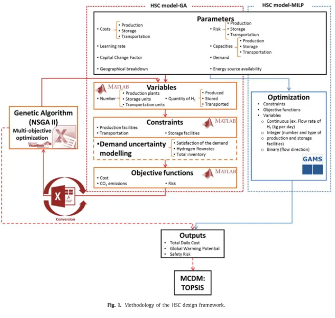
The generalmethodology ofthe HSC design proposed in this
workisillustratedin Fig.1.Itshowstheextendedflowdiagramof
the methodologyproposedforHSCdesignoptimization,
consider-ing boththemulti-objectiveoptimizationframeworkeitherbased onthedeterministicMILPsolutionstrategydevelopedin(DeLeón Almaraz, 2014)oronaGAandthemultiplecriteriadecision mak-ing tool selected to find the most interesting solution from the
compromise solutions obtained from the Pareto front based on
a variant of the TOPSIS method (Ren et al., 2007). The
MULTI-GEN environmentpreviously developed inourresearch group [8]
was selectedas thegenetic algorithm platform.The demand
un-certainty hasbeenmodelledusingfuzzyconceptsaspresentedin (Verdegay,1982, Villacortaetal.,2017).
2.2. CapturingtheHSCdesignmodelinaGAenvironment
Themathematicalmodelpreviouslydevelopedby(DeLeón
Al-maraz, 2014) for HSC design was solved within the GAMS 23.9
environment using CPLEX solver. This model has been adapted
to be embedded in an external optimization loop based on the
multi-objective genetic algorithm. The whole model is presented
to maintainits integrity,andthechangesthat havebeenadopted toconsidertheintegrationintotheexternaloptimizationloopare presentedinitalics.
2.2.1. HSCmodellingprinciples
Ageneralsupplychainnetwork(SCN)modelforhydrogen(see
Fig.2) isconsidered(productionplants,storageunits,distribution gridsanddemandforeachgrid).
Thefollowingassumptionshavebeenmade:
- Thenumberofgridsisknown(8);
- Thecapacityoftheproductionplantsandthestorageplantsis known;
Fig. 1. Methodology of the HSC design framework.
Table 2
Optimization variables and dependent variables. Optimization variables Dependent variables
NP pig AH ig GC PGWP TCC NSs ig DI ig GWP Tot PT ig TDC PR pig DL ig LC RP ig TGWP Q ilgg’ FC MC SGWP FCC NTU ilgg’ SP ig FOC PD ig ST ig
- Thedemandforeachone ofthegridsisfixedandknown(for thecrispmodel);
- Itispossibletoeitherimportorexporthydrogenfrom/toeach grid;
- Each grid can produce hydrogen in three different ways, i.e., steammethanereforming (SMR), electrolysis(centralized)and distributedelectrolysis (decentralized,i.e., produced onsitefor captiveuses);and
- Theaverage distancebetweenthe maincitiesisconsidered to calculatethedeliverydistancesovertheroadnetwork. Themathematicalmodelformulationinvolvesthefollowing no-tations:
- gandg’:gridsquaressuchthatg’6=g(8) - i:productphysicalform(LH2)
- l:typeoftransportationmodes(tankertruck)
- p:planttypewithdifferentproductiontechnologies(SMR, elec-trolysis,diselectrolysis)
- s:storagefacilitytypewithdifferentstoragetechnologies (LH2 stock)
- e: energy source type (natural gas, solar, wind, hydroelectric, nuclear)
The modelformulationis developedinthe Appendix.The
de-signdecisionsare basedon thenumber,type, capacity,and loca-tion ofproductionand storagefacilities, thenumberof transport
units, andthe flow rateof hydrogen betweenlocations. The
op-erational decisionsconcern the totalproduction rateofhydrogen ineachgrid,thetotalaverageinventoryineachgrid,thedemand coveredbyimportedhydrogenandlocalproduction.
Theinvolvedconstraintsarerelatedtodemandsatisfaction,the availability of energy sources, production facilities, storage units, transportationmodesandflowrates.
Thevariablesusedinthismodelaresplitintotwogroups: de-cisionvariablesthataregeneratedbytheoptimizationprocedure; anddependentvariablesthatarecalculatedfromtheequality con-straints.Theclassificationisshownin Table2.
2.3. Multi-objectiveoptimizationbyGAs
The solving method used in this investigation is based on a
multi-objective genetic algorithm. Let us recall that, in a single-objective optimization, theoptimalsolution isusually clearly
de-fined. However, this assumption is not the case for a
multi-objectiveprobleminwhichtheobjectivescanconflict.Asingle so-lution is hardly the best for all of the objectives simultaneously. Instead ofa singleoptimum,there isa set oftrade-off solutions,
which are the so-calledPareto optima solutions. The aim of the
multi-objectiveevolutionaryalgorithmistocausethesolutionset
to approachthe Paretoidealfrontierofthe problemwithawide anduniformdistributioninasinglesimulationrun.
A variant of the non-dominated sorting genetic algorithm II
(NSGA-II)(Debetal.,2002),whichisoneofthemostwidelyused
multi-objectiveevolutionary algorithmsimplemented throughthe
MULTIGENlibrarydevelopedby(Gomezetal.,2008),wasselected inthiswork.
The main featureofNSGA-II amongmulti-objective
evolution-ary techniques is the determination of individual fitness values
based ontheParetodominancerelationshipanddensity
informa-tionbetweenindividuals.
Inthiswork,theresultsobtainedfromthe
ε
-constraintmethod (DeLeónAlmaraz,2014)andGAarecomparedtoanalysethead-vantages anddisadvantages ofeach technique and its impact on
the network configuration of the HSC. The set of chromosomes
representingthevariablesisillustratedin Fig.3.
The variablePR representstheproductionrateofproductiby plant type p in grid g; Q is the flow rateof product iby trans-portlbetweenthegridsgandg’.NPisthenumberofproduction plantsoftypep ofproductiingridg,whileNSisthenumberof storagefacilitiesoftype pofproductiingridg.Finally,DListhe demandsatisfiedforproductibylocalproductioningridg.Inthe
GA used,thechromosomeofthe variablesiscomplementedby a
vector containing the typeof variable(i.e.,0 forcontinuous vari-ables,1forintegervariablesand2forbinaryvariables).Theother procedures followthe NSGAII variant proposed by (Gomez etal., 2008).
2.4. Multiplecriteriadecisionmaking(MCDM)
AmodifiedTOPSIS(M-TOPSIS)evaluationisbasedonthe origi-nalconceptofTOPSIS(techniquefororderofpreferenceby similar-itytoidealsolution)andproposedby(Renetal.,2007)isused.It choosesanalternativethatshouldsimultaneouslyhavetheclosest distancefromthepositiveidealsolutionandthefarthestdistance fromthenegative idealsolution,solvingtherankreversalandthe evaluation failure problempresentedin theoriginal TOPSIS tech-nique.
2.5. Uncertaintymodelling 2.5.1. Fuzzy-constraintproblems
The review proposed by (Ebrahimnejad and Verdegay, 2016)
has reportedthat manyworkshavebeendevoted tofuzzy linear
programming (FLP) andsolution methods. These worksare
typi-callydividedintofourareas:(FLP1)linearprogramming(LP) prob-lems with fuzzyinequalities andcrisp objective function; (FLP2) LP problemswith crispinequalities andfuzzyobjective function;
(FLP3) LP problems with fuzzy inequalities and fuzzy objective
function; and (FLP4) LP problems with fuzzy parameters. In the
HSC design problem that has been mathematically formulated
(DeLeónAlmaraz,2014),hydrogendemandhasbeenidentifiedas an uncertainparameter,andtheHSCdesignproblemreferstothe simplestformoffuzzylinearprogramming,i.e.,FLP1.
Thedecisionmakercanacceptaviolationoftheconstraintsup to acertaindegreepreviously established.Thisacceptancecanbe formalizedforeachconstraintas(Villacortaetal.,2017):
aix≤fbi,i=1,...,m
6
Fig. 4. Uncertain demand modelling.
In thisexpression, thef indexindicates that the inferior rela-tionshipinvolvesfuzzynumbers.
Thisindexcanbemodelledusingamembershipfunction:
µ
i:R→[0,1],µ
i(
x)
=(
1 i fx≤b i fi(
x)
i fbi≤x≤bi+ti 0 i fx≥bi+tiwhere the fi are continuous, non-increasing functions. The toler-ance thatthedecisionmakeriswillingtoaccept uptoavalue of
bi+ti is given by the membership function
µ
i. For every x ∈ R,µ
i(x)represents the degree of fulfilment of the i-th constraint.Then,theproblemcanbesolved: maxz=cx
subjectto Ax≤fb x≥0
Theapproachproposedby(Verdegay,1982)throughthe
repre-sentationtheoremhasprovedthattheproblemcanbe solvedvia
thefollowingparametriclinearprogrammingproblem: maxz=cx subjectto Ax≤g
(
α
)
x≥0,α
∈[0,1] whereg(
α
)
=(
g1(
α
)
,...,gm(
α
)
)
∈Rm,withg i=fi−1.Tosimplifytheproblem,iffiarelinear: maxz=cx
subjectto Ax≤b+t
(
1−α
)
x≥0,
α
∈[0,1]witht=
(
t1,...,tm)
∈Rm.Ithasbeenproved(Delgadoetal.,1993)that,whenfiislinear, a solutionforthefuzzyconstraintsproblemcan befound asifit is a modelwithnon-linearfunctions, without anygeneralityloss
when assuming linear functions for the fuzzy constraints. Some
samplevalues canbe applied to
α
inthe interval [0,1],andthenthe model can be solved forevery sample value. For example,a
stepsizeof0.25forsampling
α
canbetransformedinfiveα
-cuts forα
={
0;0.25;0.5;0.75;1}
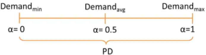
.2.5.2. ApplicationtodemanduncertaintymodellinginHSCNdesign
Hydrogendemandistheonlyparameterthatwillbeconsidered uncertain.Inthispaper,onlythemodificationsimplementedinthe HSCmodelarepresented(see Fig.4).
Theuncertaintyhasbeenconsideredusingthefollowing infor-mation:
- Thelowerandupperlevelsofdemandhavebeenobtainedfrom theanalysisin(DeLeónAlmaraz,2014);
- Fromthesevalues,averagedemandiscalculated;
- Thedifferencebetweenthe averageandthelow/highdemand
iscalculated,representinganacceptedtolerance;and
- Variable
α
is then introduced. This variable can take values from 1 to 0,andit represents the rateof useof tolerance. A valueofα
equalto0.5correspondstotheaveragedemand. Theconstraintsthataremodifiedintheinitialcrispversion of themodelareconstraints2-4.Consideringthedemandastherightsideoftheconstraints,as inVerdegays’approach (Verdegay,1982), thefuzzyrightsidecan beexpressedmathematicallyas:
g DTig=
£
DTig+PDig
(
1−α
)
¤
(1)Eq.(1)mustbeinsertedintoconstraints (2)-(4), whichreplace
the corresponding ones in the initial model (see (De León
Al-maraz,2014)). DLig+DIig=DTig+PDig
(
1−α
)
∀
i,g (2) PTig− X l,g′¡
Qilgg′−Qilgg′g¢
=DTig+PDig(
1−α
)
∀
i,g (3) STigβ
=DTig+PDig(
1−α
)
∀
i,g (4)PDig is the tolerance of DTig, and
α
is the rate of useof the tolerance. Six values of
α
-cuts were considered:α
={
0.16;0.33;0.5,0.66;0.83;1}
. Foreach value ofα
-cuts, an eval-uationofthemodelwasperformed.3. Casestudy
3.1. ParametersoftheHSC
3.1.1. Estimationofhydrogendemand
The case study refers to the design for an HSC in the
for-mer Midi-Pyrénées region in France as previously presented in
(De León Almaraz, 2014). The demand is considered
determin-istic for the first case and is calculated from the work of
(McKinsey&Company, 2010) with the same methodology as
pro-posed in (De-León Almaraz et al., 2014). The demand evolution
profile corresponds to the valuesof Dmin (Table 3) (low demand scenario studied in (De-León Almaraz etal., 2014)).The demand (for both Dmin and Dmax) includes fuel cell electric vehicles and
captivefleets(i.e.,buses,privateandlight-goodsvehicles,forklifts)
asdefined in(De León Almaraz, 2014). The market demand
sce-nariosareestablishedfrom(Bento,2010)and(McKinseyand Com-pany 2010), in which the two scenarios identifying the two lev-elsofdemandsforFCEVpenetrationweredevelopedprovidingthe
Table 3
Demand scenarios of FCEV penetration.
Scenario/year 2020 2030 2040 2050 D min 1% 7.5% 17.5% 25%
Table 4
Demand (D min , D max ) and tolerance (PD) evolution profile used in the case study (kg per day).
Period/Grid 1 2 3 4
Dmin Dmax PD Dmin Dmax PD Dmin Dmax PD Dmin Dmax PD 2020 502 995 493 843 1650 807 977 1953 976 709 1404 695 2030 3780 7440 3660 6320 12430 6110 7410 14630 7220 5320 10450 5130 2040 8850 17350 8500 14750 29030 14280 17330 34100 16770 12400 24380 11980 2050 12610 24790 12180 21100 41470 20370 24770 48730 23960 17710 34810 17100
Period/Grid 5 6 7 8
Dmin Dmax PD Dmin Dmax PD Dmin Dmax PD Dmin Dmax PD 2020 570 1136 566 639 1263 624 3221 6362 3141 437 810 373 2030 4420 8590 4170 4850 9510 4660 24180 47670 23490 3150 6250 3100 2040 10260 20030 9770 11310 22160 10850 56470 111230 54760 7420 14570 7150 2050 14610 28610 14000 16170 31660 15490 80620 158950 78330 10580 20790 10210
percentageofFCEVexpectedtoreplaceICEs(ignition combustion engines).
The hydrogen demandfor thetwo scenarios is obtainedfrom
Eq.(5)(AlmansooriandShah,2006),(MurthyKondaetal., 2011):
DTig=
(
FE)
(
d)
(
Qcg)
(5)wherethetotal demandineach grid(DT) isprovidedby thefuel economyofthevehicle(FE),theaveragedistancetravelled(d)and thenumberofFCEVsineachgrid(Qc).
Foruncertaindemand, Table4alsopresentsthedemandinthe
highdemand scenario caseproposed by (De-León Almarazet al.,
2014),i.e.,(Dmax).Thetolerancesarerepresentedbythedifferences
betweenDmaxandDminovertheperiods.
3.1.2. Techno-economicassumptions
Thestudyisbasedonthefollowingassumptions:
- acapitalchange factor(depreciationperiod)of12 yearsis in-troduced;
- in a multi-periodapproach, four periods were analysed, from 2020to2050,witha10-yeartimestepforeach;
- three types of technologies to produce hydrogen are
consid-ered: steam methane reforming (SMR), electrolysis and
dis-tributedelectrolysis;
- fiveenergysourcesare considered:solar, wind,hydro,nuclear andnaturalgas(OchoaRoblesetal.,2018);
- hydrogenmustbeliquefiedbeforebeingstoredordistributed;
- aminimumcapacityofproductionandstorageequalto50kg
ofH2 perdayisconsidered;
- renewableenergyisdirectlyusedonsitebecauseofgrid satu-ration,whichallowstoallocatetheCO2impactoneachsource;
- onesizeforstorageandproductionunitsisconsidered; - inter-districttransportisallowed;
- the maximum capacity of transportation is fixed at 3500 kg
liquid-H2(Dagdouguietal.,2012);
- thehydrogenisstoredinliquidform,anda10-dayLH2safety stockisconsidered;
- the risk indexis calculated by the methodology proposed by
(KimandMoon,2008);
- thenumberofplantsisinitializedatanullvalue;
- thecostofswitchingfromacurrentrefuellingstationtoH2fuel
isnotconsidered;and
- thelearningratecostreductionsdueaccumulatedexperienceis consideredas10%perperiod(McKinseyandCompany2010).
3.2. Optimizationparameters
For the mono-period andmono-objective case, a total of 500
individualsinthepopulationand1000generationsareconsidered, with0.9forthecrossoverrateand0.5forthemutationrate.These values havebeenfixedfroma preliminarysensitivityanalysis. As alreadyhighlighted,thedefinitionofvariablesisdifferentinboth
models. In the GA formulation, there are 352 decision variables
versus676intheMILPformulation.Inthecaseofmulti-periodand multi-objective formulations, 2000 individuals in the population and3000generationsareused,with1408variablesversus3319in the MILPmodel.FortheM-TOPSISanalysis(Renetal.,2007),the sameweighting factorsforcost,safety,andenvironmentalcriteria are considered.The defaultfeasibilityofCPLEXandtheoptimality tolerancesof10−6havebeenadopted.
4. Results
In Sections4.1to 4.3,thesamecostdataasthoseusedin( De-LeónAlmarazetal.,2014)areadoptedforvalidationpurposes.The
parameters oftheHSC modelarepresentedinthesupplementary
materials.Inallofthemapsprovided,thenumberofplantsis in-dicatedinsidethesymbolsusedfortechnologyrepresentation.The mapsareobtainedafterthesuccessiveuseoftheoptimization al-gorithmandtheMCDMstrategyforthemulti-objectivecase.
For themono-periodoptimization runs(Sections4.1and 4.2), thedemandscenariorelativetoperiod4isanalysed.
4.1. Mono-objectiveandmono-periodoptimization
A preliminarystudywasperformedwiththeGA approach:10
runswereperformedforeachcasetoguaranteethestochastic na-tureofthealgorithm(Table5).Thesamemethodologyisusedfor allofthecasesinwhichtheGAmethodologyisused.
Table 5
Statistical results of the runs performed in the mono-period and mono-objective GA approach.
Min (TDC) Min (GWP) Min (Risk)
TDC (M$/ day) GWP (ton CO 2
eq / day) Risk TDC (M$ / day) GWP (ton CO eq per day) 2 Risk TDC (M$ / day) GWP (ton CO eq / day) 2 Risk Mean 1.21 1552.08 496 1.32 763.42 485 1.22 1642.82 479 Standard deviation 0.0327 257.38 21.17 0.0218 167.42 22.17 0.0251 211.80 11.98
Table 6
Mono-objective and mono-period detailed optimization results.
The results of the three mono-objective optimizations (min
TDC,GWP,andRiskseparately),solvedbyCPLEX,ontheonehand, and by the GA,on the other hand,are presented in Table6. For
each criterion to be optimized, each column presents the
opti-mized values ofthe decisionvariables, some intermediate values involved inthe evaluationofthecriteria andtheoptimizedvalue of theconsidered criterion (inbold type andincolour). Foreach mono-optimizationcase,acomputationoftheothercriteriaisalso performedinparallel.
Table6alsopresentstheunitcostofH2 aswellastheamount ofemittedCO2 perkgofH2 thatisdeducedfromthevalueofthe optimizationcriteria(inthesamecolour).
It can be observed that, whichever criterion is considered,
CPLEXoutperformsGA.
Forinstance,whenTDCisminimized,alowervalueisnot
sur-prisingly obtained with CPLEX(1.18 M$/day) than with GA (1.21
M$/day),whichisexactlythesametrendwiththeothercriteria.
Let usconsideronce morethe TDC caseminimization forthe
sake of illustration. Since a better value has been obtained with
MILPforTDC,thevalue ofGWPisnowhigherthanthatobtained
withGA(respectively,10.82kgCO2-eqperkgH2withMILPvs7.83
kgCO2-eqperkgH2withGA),reflectingacompromiseamongthe
criteria. Thistype of observationis not valid inthis caseforthe riskcriterion,whichcanbeexplainedbydifferentuseoftransport betweenthegrids.
The trend observed for TDC can be generalized to the other
criteria:it meansthat,ifabetter valueissystematically obtained withMILPthan withGA foragivencriterion thathasbeen opti-mized,theperformanceofonecriterionthatisnotoptimizedcan bedegradedcomparedtotheresultsobtainedwithGAinthesame conditions.
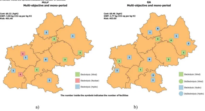
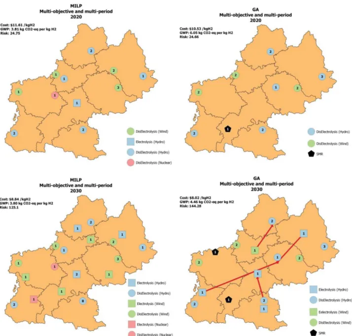
Fig. 5 showsthe obtained networkfor the three optimization
cases.ForTDCminimization,thenetworksobtainedareveryclose
to each other with both optimization strategies, producing the
most hydrogen via SMR with some electrolysis plants. The main
difference between the approaches mostly involves the way in
whichhydrogenisdistributedthroughthegrids.
When GWP is minimized, priority is given to the production
of hydrogen via electrolysis forboth approaches. With the MILP
model,thereisnotransportbetweengrids,andhydrogen produc-tionisachievedthroughseveraldistributedplants.WithGA,fewer facilitiesareinstalled,buthydrogentransportationoccursthrough grids.
Table 7
Best trade-off solutions selected by TOPSIS for ε-constraint and AG. MILP GA Demand (t per day) 198.17 198.17 Number of total production facilities 25 39 Number of total storage facilities 214 214 Number of transport units 0 0
Capital cost
Plants and storage facilities (10 6 $) 2595.00 2480.45
Transportation modes (10 6 $) 0 0
Operating cost
Plants and storage facilities (10 3 $ per day) 1056.20 1143.28
Transportation modes (10 3 $ per day) 0 0
Total daily cost (10 6 $ per day) 1.65 1.68
Cost per kg H 2 ($) 8.32 8.48
Production facilities (t CO 2 -eq per day) 614.33 409.82 Storage facilities (t CO 2 -eq per day) 139.51 139.51
Transportation modes (t CO 2 -eq per day) 0 0
Total GWP (t CO 2 -eq per day) 753.84 549.33 Kg CO 2 -eq per kg H 2 3.80 2.77
Production facility risk 14.40 16.05 Storage facility risk 387.00 387 Transportation modes risk 0 0
Fig. 6. Maps of the two scenarios with multi-objective optimization a) with GA; b) with MILP.
Forriskminimization,hydrogenproductionisbasedexclusively
onSMRplantsfortheMILPapproachandamixofSMRand
elec-trolysis for the GA approach with transportation through grids.
Thissituationismainlyduetothesmalldifferenceintherisk val-uesbetweenthevarioustechnologiesfortheplantsizethatis con-sidered.
Itmustbeemphasizedthatthesolarsourceiseliminatedinthe optimizationprocesssincehydrogenproducedviaelectrolysiswith solar energyis themostexpensiveprocess andexhibits a higher carbonfootprint,comparedtowindandhydro.
4.2. Multi-objectiveandmono-periodoptimization
In this case, the obtained results are only slightly improved withlinearprogramming,comparedtoGAforcostandriskcriteria (Table7, Fig.6(a)and(b)).The degreeofcentralizationisalmost the same. In Fig.6 (a), relative to GA, the configurationinvolves a setofseveralplantswiththedistributedelectrolysistechnology withnotransportation;withMILPin Fig.6(b),priorityisgivento electrolysisplantsfromvarioussources,includingthenuclearone (see Table8).
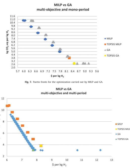
The Pareto solutions proposed by the GA include the Pareto
space, which was identified as using the MILP methodology
(Fig.7).Asmallvariation(2%)isobservedintheunitcost($8.32of MILPvs$8.48perkgH2ofGA)betweenthetwoTOPSISsolutions.
From the environmental viewpoint, a significant improvement is
observed withtheGA:GWPexpressedinkgCO2 eqper kgH2 in
the GA approach is 27% lower than the value obtained withthe
Table 8
Use ratio of energy sources for hydrogen production (multi- objective and mono-period case).
Energy source MILP GA Wind 60% 69% Hydraulic 32% 31% Nuclear 8% 0%
MILPapproach.Thisdifferencecanbeexplainedbytheuseof dis-tributedplantsinsteadofelectrolysisplants.The differenceinthe riskcriteriabetweentheapproachesisnotsignificant.
The computation time for MILP withCPLEX (Intel R
°
Xeon R°
CPU 2.10GHz) is approximately3 hours versus 4 hours with GA,
withasetof174ParetopointsobtainedwiththeGAapproachand 43withtheMILPapproach.
4.3.Multi-objectiveandmulti-periodoptimization
Fig. 8 is a projection of the Pareto surface onto the
two-dimensional plane corresponding to cost and environmental
im-pact. Forthese two criteria, better compromise solutions are ob-tainedwiththeGAthanwithCPLEX.Thiscaseisnottruewiththe riskindex,whichcanbehigher.
TheTOPSISsolutions(see Table9)providelowervaluesforboth
costandGWP.The unitcost ofhydrogenislower withGA(8.00)
thanwithMILP(8.27),despitea slightlyhigherrisk (838vs873). Thisoutcomecanbeexplainedbythewayinwhichtheplantsare distributedthroughtheperiods.
IntheMILPapproach(Fig.9),priorityisgiveninthefirstperiod tothe establishmentofdistributedplants,mainlydueto thelow
value of the demand. In the three other periods, the demand is
satisfiedmainlywiththeelectrolysisplantssothatGWPandrisk remainnotashigh.
IntheGAapproach(Fig.9),thefirstperiodisdedicatedtothe installationofdistributedelectrolysisplantsandoneSMR, signifi-cantlyincreasingCO2emissions.Forthesecondperiod,some
elec-trolysis plantsare added. The CO2 emissions remain higherthan withMILP, andbecause of transport betweengrids, therisk also increases.Forthethirdandfourthperiods,transportbetweengrids remains,buttheSMRplantsdisappearfromdistribution, decreas-ingtheCO2emissions.
Finally,forthisexampleandwithoutprovidingafeatureof gen-eralitytotheobtainedresults,comparedtoMILP,GApromotesthe deployment of hydrogen by favouring cost objectives inthe first period.Inthelasttwoperiods,bettervaluesforGWPareobtained withtheGAapproachratherthanwithMILPbecauseofthe
instal-Fig. 7. Pareto fronts for the optimization carried out by MILP and GA.
Fig. 8. Projection of the Pareto fronts onto the two-dimensional plane corresponding to cost and environmental impact for the optimization run carried out by MILP and GA for a multi-objective and multi-period approach.
lationof asmaller numberofproductionfacilities. Thisapproach
leads againto the implementationof transport between grids to
satisfy the demand. Finally, fromthe safety point of view (risk), theMILPmodelpresentsbetterresults,mostlyduetotheabsence oftransport betweenthegrids. Table10showsthepercentageof
energy sources used by each methodology. Regarding the
mono-objective case, the solarsource is eliminated in theoptimization process.
4.4. Multi-objectiveandmulti-periodoptimizationwithnewcosts
Inadditiontohydrogendemand,oneofthemostsignificant pa-rametersisfeedstockcost(OchoaRoblesetal.,2017),(Ochoa Rob-les et al., 2017). In the original model (De-León Almaraz et al., 2014),the unit production cost(UPC) of electricity remains fixed for all of the periods regardless of the technology, which was a severesimplification.Inwhatfollows,anevaluationofUPCis con-sideredwithfixedfacilitycosts(maintenance,labourcost),aswell aselectricityandfeedstockcosts.
Table 11presentsthepriceofelectricityproducedfrom differ-ent energysources andthe priceofnaturalgas forconditionsin France(2013).
In the original model,UPC is a fixed parameter (De León Al-maraz, 2014) (SMR: $3.36 per kg; electrolysis: $4.69per kg; dis-electrolysis $6.24per kg), whichis only dependenton the size of the productionunit ($per kgH2). However, asmentionedinthe (McKinsey&Company,2010)report,abettervisionofUPCisto con-siderthefixed,electricityandfeedstockcosts.Thefixedcostis re-latedtolabourandmaintenance.
Allofthecontributionsarereflectedin Eq.(6),wheretheUPC calculation($perkgH2)isgivenbytheadditionofthefixedcost
ofaproductionplantoftypepandsizejintimeperiodt(FCPept,
$per kgH2),theelectricitycostforgeneralusageinaproduction plantoftypepprojectedfortimeperiodt(ECept,$perkgH2)and
the feedstockecostfora productionplantofthe ptype (FSCept).
The FSCept isobtainedbymultiplying thefeedstockeefficiencyin
the process p intime t (kWhelec/kg H2) by thefeedstock e price
consid-Table 9
Multi-objective and multi-period optimization results.
MILP GA
Year 2020 2030 2040 2050 2020 2030 2040 2050 Demand (t per day) 7.90 59.43 138.79 198.17 7.90 59.43 138.79 198.17 Number of total production facilities 17 34 47 69 17 28 30 41 Number of total storage facilities 12 66 150 214 12 66 150 214
Number of transport units 0 0 0 0 0 4 2 3
Capital cost
Plants and storage facilities (10 6 $) 681.01 765.69 707.92 185.42 737.93 520.31 443.72 153.42
Transportation modes (10 6 $) 0 0 0 0 0 0.80 0.28 0.41
Operating cost
Plants and storage facilities (10 3 $ per day) 49.35 321.64 748.23 1066.00 48.14 332.99 786.41 1133.53
Transportation modes (10 3 $ per day) 0 0 0 0 0 1.31 0.46 0.46
Total daily cost (10 3 $ per day) 91.68 525.60 1127.00 1600.25 83.17 476.53 1116.65 1557.90
Cost per kg H 2 ($) 11.61 8.84 8.12 8.08 10.53 8.02 8.05 7.86
Production facilities (t CO 2 -eq per day) 24.58 185.23 430.25 613.33 42.20 220.70 287.02 409.82 Storage facilities (t CO 2 -eq per day) 5.56 41.84 96.71 139.51 5.56 41.84 97.71 139.51 Transportation modes (t CO 2 -eq per day) 0 0 0 0 0 2.60 2.19 1.44 Total GWP (t CO 2 -eq per day) 30.14 226.07 526.96 752.84 47.76 265.13 386.91 550.77
Kg CO 2 -eq per kg H 2 3.81 3.80 3.79 3.79 6.05 4.46 2.79 2.78
Production facility risk 4.05 6.30 12.45 16.05 3.96 4.68 9.60 13.50 Storage facility risk 20.7 118.8 272.7 387 20.7 118.8 272.7 387 Transportation modes risk 0 0 0 0 0 20.8 6.5 14.3 Total Risk 24.75 125.10 285.15 403.05 24.66 144.28 288.80 414.80
Global TDC (M$ per day) 3.34 3.23
Global unit cost ($ per kg H 2 ) 8.27 8.00
Global GWP (T CO 2 eq per day) 1536 1251
Global Kg CO 2 -eq per kg H 2 3.80 3.09
Global Risk 838 879
Table 10
Use ratio of energy sources for hydrogen production (multi-objective and multi-period case).
Energy source MILP GA
2020 2030 2040 2050 2020 2030 2040 2050 Natural gas 0% 0% 0% 0% 6% 11% 0% 0% Hydro 53% 71% 70% 64% 53% 67% 70% 64% Wind 41% 24% 30% 36% 41% 22% 30% 36% Nuclear 6% 6% 0% 0% 0% 0% 0% 0% Table 11
Prices of natural gas and costs of electricity from different sources (2013).
Energy source (Price/unit) 2020 2030 2040 2050 Reference
European price of natural gas ($2010/kg) 0.587 1.300 1.750 ∗ 2.200 For 2030 and 2050: [48]
Cost of electricity (nuclear) in France
( $2013/kWh ) 0.0439 0.0665 0.089
∗ 0.112 ∗ For 2020: [49]
For 2030: [50] Cost of electricity (PV) in France ( $2013/kWh ) 0.328 0.101 0.060 ∗ 0.053 For 2020: [49]
For 2030 and 2050: [51] Cost of electricity (Wind) in France ( $2013/kWh ) 0.073 0.068 ∗ 0.063 ∗ 0.058 For 2020: [49]
For 2050: [51] Cost of electricity (Hydro) in France ( $2013/kWh ) 0.018 0.044 ∗ 0.071 ∗ 0.098
∗ Calculated by interpolation.
erediselectricity,andtheenergysourcecostvariesdependingon thetype,e.g.,fossilvsrenewable(Table11).
UPCe,p,t=FCPe,p,t+ECe,p,t+FSCe,p,t (6)
The feedstock cost is likely togain importance becauseit de-pendsontheenergytransitionscenarioandinducesacostchange
in renewable energy impacting the hydrogen cost overthe
long-timehorizonfrom2020to2050.
ThenewUPCcalculatedforthemodelispresentedin Table12, in which hydrogenproduced via electrolysiswith solarenergyis
the most expensive, while hydrogen produced with electrolysis
fromahydraulicsourceislessexpensive.
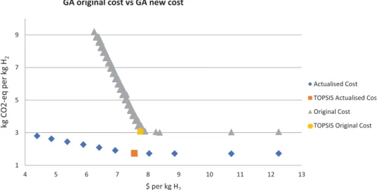
Theoptimizationrunsareperformedwiththesenewcosts,and the resultsare compared withthe previous ones (see Fig. 10). A
strong decrease in GWP is observed for the range of these new
costs,globallyleadingtobettersolutionsforallcriteria.
In the first period (see Fig. 11 and Table 13), the distributed plantsarethemainsourcesofproduction,whileintheother peri-ods,the electrolysisplantsstartedto beinstalled inthe different grids. Additionally, there is no transport between grids, and the CO2 emissions for the plants installed remain very low. Most of
Fig. 9. Maps of the four scenarios for the optimization run carried out by MILP and GA for a multi-objective and multi-period approach.
Table 12
UPC calculated with the new costs. Production technology Fixed cost of production ($ per kg H 2 ) Electricity usage of production plant ($ per kg H 2 ) Feedstock cost for production plant ($ per kg H 2 ) Electrical need to produce a kg of H 2 kWh elec /kg H 2
Cost of energy source ($ per kg H 2 ) ∗ UPC ($ per kg H 2 )
2020 2030 2040 2050 2020 2030 2040 2050 SMR 0.16 0.02 4.02 ¥ 3.71 2.61 3.46 4.62 3.89 2.79 3.64 4.80 Electrolysis PV 0.39 0.06 55 18.04 5.56 3.30 2.93 18.49 6.01 3.75 3.38 Wind 0.39 0.06 55 4.00 3.72 3.45 3.17 4.45 4.17 3.90 3.62 Hydro 0.39 0.06 55 0.98 2.44 3.90 5.36 1.43 2.89 4.35 5.81 Nuclear 0.39 0.06 55 2.41 3.66 4.90 6.14 2.86 4.11 5.35 6.59 Dis Electrolysis PV 0.75 0.11 55 18.04 5.56 3.30 2.93 18.90 6.42 4.16 3.79 Wind 0.75 0.11 55 4.00 3.72 3.45 3.17 4.86 4.58 4.31 4.03 Hydro 0.75 0.11 55 0.98 2.44 3.90 5.36 1.84 3.30 4.76 6.22 Nuclear 0.75 0.11 55 2.41 3.66 4.90 6.14 3.27 4.52 5.76 7.00
∗[Energy source cost ($/KWh)x Electrical need to produce a kg of H
2 (kWh elec /kg H 2 )].
Fig. 10. Pareto fronts obtained with the original GA and the GA with the new cost.
Table 13
Multi-objective and multi-period results for actualised costs. GA new costs
Year 2020 2030 2040 2050
Demand (t per day) 7.90 59.43 138.79 198.17 Number of total production facilities 25 62 92 110 Number of total storage facilities 12 66 150 214 Number of transport units 0 0 0 0
Capital cost
Plants and storage facilities (10 6 $) 304.47 401.53 263.71 43.44
Transportation modes (10 6 $) 0 0 0 0
Operating cost
Plants and storage facilities (10 3 $ per day) 43.44 307.15 708.68 1013.16
Transportation modes (10 3 $ per day) 0 0 0 0
Total daily cost (10 3 $ per day) 80.12 489.34 1036.96 1446.56
Cost per kg H 2 ($) 10.14 8.23 7.47 7.30
Production facilities (t CO 2 -eq per day) 8.27 61.35 142.51 201.91
Storage facilities (t CO 2 -eq per day) 5.56 41.84 97.71 139.51 Transportation modes (t CO 2 -eq per day) 0 0 0 0
Total GWP (t CO 2 -eq per day) 13.73 103.18 240.22 341.42
Kg CO 2 -eq per kg H 2 1.74 1.74 1.73 1.72
Production facility risk 7.20 9.00 12.45 20.55 Storage facility risk 20.7 118.8 272.7 387.0 Transportation modes risk 0 0 0 0 Total Risk 27.90 127.80 285.15 407.55 Global TDC (M$ per day) 3.05
Global unit cost ($ per kg H 2 ) 7.55 Global GWP (T CO 2 eq per day) 698
Global Kg CO 2 -eq per kg H 2 1.73
Global Risk 848
Table 14
Use ratio of energy sources for hydrogen production (with new costs).
Energy sources 2020 2030 2040 2050 Hydro 22% 30% 22% 33% Wind 78% 70% 78% 67%
theenergysources usedstemfromwind,withalmost 70%ofthe
electricityproduced(Table14).
4.5. Multi-objectiveGAapproachunderuncertaindemand
In thiscase, the demand can vary betweenlow andhigh
de-mand(DminandDmax,respectively, in Table4).The toleranceis
thedifferencebetweenthetwolevelsofdemand,and
α
isthe per-centageoftolerancethatisaddedtothebasedemand(Dmin). Sev-eralvaluesofα
areused(see Table15),andthedemandusedfor eachα
-cutdependsonthetolerancelevel.For each
α
-value, a tri-criterion optimization procedure withthe GA procedure is implemented, leading to the set of
solu-tions constituting theParetofront, towhichthe M-TOPSIS proce-dure is then applied. The criteria (average values over the peri-ods) relative tothe compromise solution ofthe HSCN finally ob-tainedarepresentedin Table16,andtheinstancesobtainedfor
α
equal to 0; 0.16;0.33;and 0.50are shownin Table 17,in which the relative deviation relative to the case
α
equal to 0 case is presented.Table 15
Table 16
Results of HSCN solutions the different α-cuts (average values over the period).
Table 17
Table 18
Robustness analysis of the optimal configurations.
α= 0.33 α= 0.66 α= 1
2020 2030 2040 2050 2020 2030 2040 2050 2020 2030 2040 2050 TDC (M$ per day) 89.24 514.66 1083.21 1494.42 93.31 554.59 1193.17 1614.67 98.93 593.65 1292.13 1729.73
Relative deviation (reference α= 0) 11% 5% 4% 3% 16% 13% 15% 12% 23% 21% 25% 20%
Unit cost ($ per kg H 2 ) 11.30 8.66 7.80 7.54 11.81 9.33 8.60 8.15 12.52 9.99 9.31 8.73
relative deviation (reference α= 0) 11% 5% 4% 3% 16% 13% 15% 12% 24% 21% 25% 20%
GWP (T CO 2 eq per day) 13.83 103.19 240.22 341.42 13.85 103.51 241.02 341.98 13.74 102.96 240.52 341.55
relative deviation (reference α= 0) 0% 0% 0% 0% 0% 0% 0% 0% 1% 0% 0% 0%
GWP (kg CO 2 eq per kg H 2 ) 1.74 1.74 1.73 1.72 1.75 1.74 1.74 1.73 1.74 1.73 1.73 1.72
relative deviation (reference α= 0) 0% 0% 0% 0% 1% 0% 0% 0% 0% 0% 0% 0%
Risk 45.25 278.12 602.26 821.36 70.31 326.36 749.19 1064.64 94.76 373.11 764.79 1099.59
relative deviation (reference α= 0) 62% 118% 111% 102% 152% 155% 163% 161% 240% 192% 168% 170%
Fig. 12. Cost of hydrogen in 2050 ($ per kg H 2 ). As expected, the operating cost and the capital cost increase
with hydrogen demand.Although the TDC is higherwhen
α
in-creases,theunit costdecreases,mostlyduetotheeffectofscale. For example, in the first period (2020), with a value of
α
equal to0(respectively0.5),theunitcostofH2 is$10.14/kgH2(respec-tively$6.98/kgH2).Thesamesituationisobservedoverthewhole
period.Conversely,GWPandriskincreasewithhydrogendemand.
Thenumberoffacilitiesalsoincreasesas
α
-valueincreases, ex-cept forα
equal to0.5, forwhich priorityisgiven toelectrolysis plantsinsteadofdistributedones,allowing forgreatercapacityto beavailable.Arobustness studycanthus beperformedfromthe
optimiza-tion resultspresentedin Table18.LetusconsidertheHSCN con-figurationobtainedwith
α
equalto 0.33.Thenetwork,whichhas beenobtained fromthesuccessiveuse ofthemulti-objectiveop-timization procedures andMCDM techniques, is perfectly
consis-tentwiththecorrespondingdemand.However,ifthedemanddoes
notreachthemaximalexpectedvalue,itwillresultinhigher val-uesfor allcriteria. Tocheck whetheran acceptable rangeforthe criteria valuescan still be obtained even if the network is over-dimensionedforthisdemandlevel,apost-optimalanalysisisthen
performed using the given network and the lowest value of the
demand. Table18comparestheresultsobtainedinbothscenarios.
4.6. Resultsanddiscussion
Thehydrogenpriceevolutionisdirectlydependenton produc-tion anddistribution costs. The differentstudies have shownthe
hydrogencost evolutionwiththegradualintroductionofdemand
fromthemobilitysector. Acomparativestudyofthe different re-sults considering different FCV market penetration rates, consid-ering differenthydrogen production technology choices, was car-ried out,andeven forthehighestdemand,theresultsshow (see
Fig. 12)that hydrogencosts for2050remainexpensivecompared
to the Hyways roadmaptargets (European Commission 2008) for
thebestcompromisesolutionsobtainedusingtheproposed multi-objective-MCDM framework. Forthe sake ofillustration, the best solutionobtainedforhydrogencostminimization ($4.18/kgofH2)
and GWP minimization ($7.30/kg H2) has also been reported. A
consistent approach wouldbe to find acompromise solution
be-tweentheseboundssincetheGWPisconsistentwiththetargeted values(Mobilité HydrogèneFrance2016)(see Fig.13).
Fig.13 comparesthewell-to-wheel CO2 emissionsper km
ob-tained withFCEVs obtainedby the useof theproposed
method-ology and those related to ICE vehicles equipped with
gasoline-ordiesel-fuelledengines(HydrogenCouncil2017)forthe2050 pe-riod.Currently,on-roadfueleconomyisapproximately1kgof
hy-drogen per 100 kmtravelled, andtheemissionsexpected forICE
vehiclesareapproximately60gCO2/km(IEA2015).Withthecosts
used intheoriginal models,theemissionsareinthe rangeof28 - 38gCO2/kmfortheMILPandGAapproaches,respectively.With thenewUPCcost,theemissionsarelessthan20gCO2/km.Itmust
be emphasized that FCEV emissionsareexpected tobe lessthan
23 g CO2/km (Mobilité Hydrogène France 2016) in 2030, which
means thattheHSCN obtainedwiththe newcosts iscompetitive
Fig. 13. Comparison of emissions by sector in 2050 (g CO 2 /km). Data from [59].
5. Conclusion
This paperhas presentedthe coremethodology forHSCN
de-sign, combining multi-objective optimization tools and multiple
criteriadecision-makingtechniques.Thescientificchallengeofthis work was to use the potential of genetic algorithms asan
alter-native to the current methodologies in the optimization of the
HSCdesign,particularlyasacomplementaryapproachtotheMILP frameworkpreviouslydevelopedin(De-LeónAlmarazetal.,2014): the size andparticularlythenumber ofbinary variableshave of-ten led to difficulties for problem solution in (De-León Almaraz et al., 2014). Inthis work, a variantof NSGA-II previously devel-oped in(Gomezet al., 2008) was explored toaddress the
multi-objective formulation sothat compromise solutions can be
auto-maticallyproduced.
The case study of the hydrogen mobility market in the
for-merMidi-Pyrenéesregionhasbeenconsideredsinceitwasalready studiedin(De-LeónAlmarazetal.,2014)forvalidationpurposesof theproposedmethodology:itisforeseentobethefastestgrowing
and most important market in the horizon of 2025 – 2030 and
thusisclearlyrelevanttothecontextofa“greenhydrogen” study. The objectivefunctionsobtainedbyGAexhibit thesameorder
of magnitudeasthose obtainedwithMILPin themono-criterion
problem, andthe multi-objectiveGAyields a Paretofrontof bet-ter qualitywithabetterdistributionofthecompromisesolutions. However, inourview,bothstrategiesdo nothavetobe opposed,
butthemaximumuseoftheirpotentialbenefitsmustbemade.
Severalexperimentswere developedwithafixeddemand and
for mono- and multi-objective cases. In the multi-objective
in-stances, the GAoutperformsthe
ε
-constraintstrategy. Itmust be emphasized thattheGA prioritizestheTDC cost,providingbetter resultsthantheε
-constraintmethod,aswellasthetransportation ofhydrogenbetweenthegrids.Thedifferencesinthedistributionsandthe resultsbetweentheGAandthe MILPapproachescan be
explained bywayofmanaging the constraintsandtheir different logics.
In the original model(De-LeónAlmaraz etal., 2014), the unit productioncost(UPC)ofelectricityremainsfixedforallofthe pe-riods, regardlessofthe hydrogentechnology, whichwas a severe simplification. Theunit production cost involvesthe fixed facility costs (maintenance, labourcost), as well as electricity and feed-stockcosts,whicharemorerelevanttotherealityofcosts.
Hydrogen demand was identified as one the most significant
parameters forHSCNdesign,andaGAmodelwasdevelopedwith
demanduncertaintymodelledusingfuzzyconcepts.
Since hydrogen demand was simply involved through
con-straints in the HSCN model formulation, the HSC design
prob-lem refers to the simplest form offuzzy linear programming, as
proposedby (Verdegay,1982),(EbrahimnejadandVerdegay,2016,
Delgadoetal., 1993).Thesolutionstrategycanthusbe easily
im-plementedby varying
α
,whichcanbeconsidered thepercentageof tolerance added to the base demand. This sensitivity analysis has allowed for identifying more robust solutions. The solutions arecomparedwiththeoriginalcrispmodels,basedoneitherMILP orGA,givingmorerobustnesstotheproposedapproach.
Anextension could be todevelop a fuzzyoptimization model
for supplychain design that considers demand andprice
uncer-tainties.Themodelcould beformulated asafuzzymixed-integer
linear programming model, in which the data are poorly known
andmodelledbytriangularfuzzynumbers.Thesynergeticeffectof
geneticalgorithmsandfuzzydemandmodellingcouldbethus
ex-ploredsothat thefuzzymodelwouldprovidethedecisionmaker
withalternativedecisionplansfordifferentdegreesofsatisfaction. Finally,thisstudyhasrevealedthat iftheeconomicand envi-ronmentalcriteriacanbeformulatedbyprovenmethodologies,the safetyriskisperhapsmoredifficulttoformulateandcalibrate.
Theuseoftheframeworkcould beusefulindeploying
hydro-gensolutionssincetheintroductionofhydrogenasanenergy car-rierisnotonlyatechnologychallenge,butitalsorequiresthe con-vergenceofmanyeconomic,environmentalandsocialfactors.
DeclarationofCompetingInterest
Allauthors have participatedin (a)conception anddesign, or analysisandinterpretationof thedata; (b)draftingthe articleor revisingitcriticallyforimportantintellectualcontent;and(c) ap-proval of the final version.This manuscripthas not been submit-tedto,norisunderreviewat,anotherjournalorotherpublishing venue.Theauthorshavenoaffiliationwithanyorganizationwitha directorindirectfinancialinterestinthesubjectmatterdiscussed inthemanuscript
Supplementarymaterials
Supplementary material associated with this article can be
found, in the online version, at doi:10.1016/j.compchemeng.2020. 106853.
Appendix
Indices
g and g’ Grid squares such that g’ 6 = g (8)
I Product physical form
L Type of transportation mode
P Plant type with different production technologies
S Storage facility type with different storage technologies
E Energy source type Parameters
B Storage holding period - average number of days’ worth of stock (days)
γepj Rate of utilization of primary energy source e by plant type p and size j (unit resource/unit product)
AD gg’ Average delivery distance between g and g’ by transportation l (km per trip)
Adj gg’ Road risk between grids g and g’ (units)
CCF Capital change factor payback period of capital investment (years) DT ig Total demand for product form i in grid g (kg per day)
DW l Driver wages for transportation mode l (dollars per hour)
FE l Fuel economy of transportation mode l (km per litre)
FP l Fuel price of transportation mode l (dollars per litre)
GE l General expenses of transportation mode l (dollars per day)
GWProd p Production GWP by plant type p (g CO 2 -eq per kg of H 2 ) GWStock i Storage global warming potential form i (g CO 2 -eq per kg of H 2 ) GWTrans l Global warming potential of transportation mode l (g CO 2 per ton-km)
LUT l Load and unload times of product for transportation mode l (hours per trip)
ME l Maintenance expenses of transportation mode l (dollars per km)
NOP Network operating period (days per year)
Qmax il Maximum flow rate of product form i by transportation mode l (kg per day)
Qmin il Minimum flow rate of product form i by transportation mode l (kg per day)
PCapmax pi Maximum production capacity of plant type p for product form i (kg per day)
PCapmin pi Minimum production capacity of plant type p for product form i (kg per day)
PCC pi Capital cost of establishing plant type p producing product form i (dollars)
RP p Risk level of the production facility p (units)
RS s Risk level of the storage facility s (units)
RT l Risk level of the transportation mode l (units)
SCapmax si Maximum storage capacity of storage type s for product form i (kg)
SCapmin si Minimum storage capacity of storage type s for product form i (kg)
SCC si Capital cost of establishing storage type s storing product form i (dollars)
SP l Average speed of transportation mode l (km per hour)
SSF Safety stock factor of primary energy sources within a grid (%)
TCap il Capacity of transportation mode l transporting product form i (kg per trip)
TMA l Availability of transportation mode l (hours per day)
TMC il Cost of establishing transportation mode l for product form i (dollars)
UPC pi Unit production cost for product i produced by plant type p (dollars per kg)
USC si Unit storage cost for product form i at storage type s (dollar per kg-day)
W l Weight of transportation mode l (tons)
WFP g Weigh factor risk population in each grid (units)
Variables
A Rate of utilization of the tolerance AH ig Available hydrogen in grid g
DL ig Demand for product i in grid g satisfied by local production (kg per day)
DI ig Imported demand for product form i in grid g (kg per day)
FC Fuel cost (dollars per day) FCC Facility capital cost (dollars)
FOC Facility operating cost (dollars per day) GC General cost (dollars per day)
GWPTot Total global warming potential of the network (g CO 2 -eq per day)
LC Labour cost (dollars per day) MC Maintenance cost (dollars per day)
NPp ig Number of plants of type p producing product form i in grid g
NSs ig Number of storage facilities of type s for product form i in grid g
NTUil gg’ Number of transport units between g and g’
PD ig Tolerance of the demand in grid g
PGWP Total daily GWP in production facility p (g CO 2 -eq per day)
PR pig Production rate of product i produced by plant type p in grid g (kg per day)
PT ig Total production rate of product i in grid g (kg per day)
Qil gg’ Flow rate of product i by transportation mode l between g and g’ (kg per day)
RP ig Received hydrogen in grid g
SGWP Total daily GWP in the storage technology s (g CO 2 -eq per day) SP ig Overproduction of hydrogen in grid g
ST ig Total average inventory of product form i in grid g (kg) TCC Transportation capital cost (dollars)
TDC Total daily cost of the network (dollars per day) TGWP Total daily GWP in transportation mode l (g CO 2 -eq per day) TOC Transportation operating cost (dollars per day)
TotalRisk Total risk of this configuration (units) TPRisk Total risk index for production activity (units) TSRisk Total risk index for storage activity (units) TTRisk Total risk index for transport activity (units)
Modelformulation
The modelis based on an optimization formulationinvolving
theeobjectivefunctions(minimizationcaseconsideredinisolation orsimultaneously)andasetofconstraints.Theconstraintsare ex-pressedforthewholetimehorizondividedintoseveraltperiods
Costobjective
Thecostobjectiveinvolvesthetotaldailycost(TDC), represent-ing thecost in $ per dayof the entireHSC, in whichFCC isthe facility capital cost ($), TCCis the transportation capitalcost ($), andNOPisthenetworkoperatingperiod(daysperyear)relatedto thecapitalchargefactor(CCF,inyears).Then,thefacilityoperating cost(FOC,$perday)andthetransportationoperatingcost(TOC,$ per day)arealsoassociated.Inaddition,thecostofimported en-ergy (UICasthe unitary imported cost andIPES asthe imported energy)isadded. TDC=
³
FCC+TCC(
NOP)
CCF´
+FOC+TOC+X eg UICeIPESeg (A.1)whereFCCisrelatedtotheestablishmentofproductionand stor-agefacilities.Itiscalculatedbytheproductoftheproductionand storageplants(NPandNS,respectively)andtheircapitalcosts(PCC
andSCC,respectively),dividedbythelearningrate,whichisacost reduction fortechnologyandmanufacturers thatresultsfromthe accumulationofexperienceduringatimeperiod.
FCC=X i,g
Ã
1 LearnRÃ
X p PCCpiNPpig+ X s SCCsiNSsig!!
(A.2)Thetransportcost(TCC)dependsontheflowratebetween dif-ferent grids (Q), the transportation mode availability (TMA), the distance betweengrids (AD) (round trip), the averagespeed (SP), the loading/unloadingtime (LUT) and the cost for transportation mode(TMC). TCC=X i,l
(
"
X i,l,g,g′µ
Q ilgg′ TMAlTCapilµ
2 ADgg′ SPl +LUTl¶¶#
TMCil)
(A.3) FOC refers tothecost forproductionandstorageplant opera-tion,dependingonunitproductionandstoragecosts(UPCandUSC, respectively)andonthequantityofhydrogenproducedandstored (PRandST,respectively). FOC=X i,gÃ
X p UPCpiPRpig+ X s USCsiSTig!
(A.4)Finally,TOCconsiders:
• fuelcost(FC),givenbythefuelpriceandthedailyfuelusage; • labourcost(LC),givenbythedriverwageandthetotaldelivery
time;
• maintenancecost(MC),representedbythemaintenanceofthe
transportationbydistancetravelled;and
• andgeneralcost(GC),consistingoftransportationinsurance,
li-censesandregistrations,andoutstandingfinances.
TOC=FC+LC+MC+GC (A.5)
Globalwarmingpotentialobjective
The global warming potential (GWPTot, in g CO2 per day) is givenbythetotaldailyproductionGWP(PGWP,ingCO2 perday),
thetotaldailystorageGWP(SGWP,ingCO2perday)andthetotal dailytransportGWP(TGWP,ingCO2perday).
GWPTOT=PGWP+SGWP+TGWP (A.6)
TheGWPrelatedtotheproductioniscalledPGWPandisgiven by the quantity of hydrogenproduced (PR) and the emissionsof CO2 associatedwiththeproductionfacilities(GWiprod.
PGWP=X pig
¡
PRpigGWiprod
¢
(A.7)The GWPassociated withthe storage isthe SGWP,where the
hydrogenproduced(PR)isrelatedtotheGWPforthestorage tech-nology(GWstock i ). SGWP=X pig
¡
PRpigGWistock¢
(A.8)The GWP associated with transport (TGWP) is given by the
distance (AD) and the flow rate of hydrogen (Q) between grids, theglobalwarmingpotential(GWiptrans)associatedwiththe trans-portationmodeanditsweight(Wl).
TGWP=X ilgg′
µ
2AD lgg′Qilgg′ TCapil
GWTrans i wl (A.9) RiskobjectiveThetotalrelativerisk(TR)(A.10)compilesTPRisk,thetotalrisk ofproductionfacilities(A.11),TSRisk,thetotalriskofstorage facil-ities(A.12),andTTRisk,thetotalriskoftransportationunits(A.13).
TR=TPRisk+TSRisk+TTRisk (A.10)
Eachiscomputedbytheproduct ofthenumberofproduction
plants(NP) (or the storageunits (NS) orthe transportation units (NTU))byariskfactor(RP,RS,andRT,respectively)andbythe pop-ulationweightfactorineachgridinwhichtheproductionor stor-agefacilityislocated(WFP)ortheroadriskbetweengrids(Adj). TPRisk=X pig
¡
NPpigRPpWFPg¢
(A.11) TSRisk=X sig¡
NSsigRSsWFPg¢
(A.12) TTRisk=X ilgg′ NTUilgg′RTlAdjgg′ (A.13) ConstraintsForinteroperabilitypurposeswiththeMULTIGENplatform,the inequality constraints have been coded in Matlab R
°
and formu-latedfollowingthe“lower orequalthanzero” structure(≤0). All of the demand (DT) must be satisfied with the local production (DL)andthehydrogenimportedfromothergrids(DI)DTig=DLig+DIig
∀
i,g (A.14)Basedonthe conservationofmass,thetotalflow ofhydrogen leavingthegridg(Q,fromgtog’)andthetotalproductionratein thesamegrid(PT)mustbeequaltotheflowofhydrogenentering thegridg(Q,fromg’tog)andtotaldemandrequiredbythesame grid(DT): PTig= X l,g′
¡
Qilgg′−Qilg′g¢
+DTig∀
i,g (A.15)Toguaranteetheavailabilityoftheproduct,avariableisadded. Duringsteady-stateoperation,thetotalinventoryofproductform
iingridg(ST)isequaltoafunctionofthecorrespondingdemand (DT)multipliedbythestorageperiod(

![Fig. 13. Comparison of emissions by sector in 2050 (g CO 2 /km). Data from [59].](https://thumb-eu.123doks.com/thumbv2/123doknet/2947657.79892/19.892.171.702.117.428/fig-comparison-emissions-sector-g-km-data.webp)