HAL Id: hal-01433778
https://hal.archives-ouvertes.fr/hal-01433778
Submitted on 10 Jan 2020
HAL is a multi-disciplinary open access
archive for the deposit and dissemination of
sci-entific research documents, whether they are
pub-lished or not. The documents may come from
teaching and research institutions in France or
abroad, or from public or private research centers.
L’archive ouverte pluridisciplinaire HAL, est
destinée au dépôt et à la diffusion de documents
scientifiques de niveau recherche, publiés ou non,
émanant des établissements d’enseignement et de
recherche français ou étrangers, des laboratoires
publics ou privés.
A Railroad Detection Algorithm for Infrastructure
Surveillance using Enduring Airborne Systems
Andrei Purica, Beatrice Pesquet-Popescu, Frederic Dufaux
To cite this version:
Andrei Purica, Beatrice Pesquet-Popescu, Frederic Dufaux. A Railroad Detection Algorithm for
In-frastructure Surveillance using Enduring Airborne Systems. The 42nd IEEE International Conference
on Acoustics, Speech and Signal Processing (ICASSP 2017), Mar 2017, New Orleans, United States.
�10.1109/icassp.2017.7952544�. �hal-01433778�
A RAILROAD DETECTION ALGORITHM FOR INFRASTRUCTURE SURVEILLANCE
USING ENDURING AIRBORNE SYSTEMS
Andrei I. Purica
?†, Beatrice Pesquet-Popescu
?, Frederic Dufaux
?,
?
LTCI, CNRS, T´el´ecom ParisTech, Universit´e Paris-Saclay, 75013, Paris, France
†University Politehnica of Bucharest,061071, Romania
Email:{purica, pesquet, [email protected]
ABSTRACT
Infrastructure surveillance is an important requirement for many companies. With the advancement of technology, drones can now provide an efficient tool for such applications. A possible future sce-nario is the automated surveillance of railroads. Whereas numerous algorithms that provide railroad detection exist, they have mainly focused either on satellite images or for small, low altitude drones which are unsuitable for our particular scenario. In this paper we propose a railroad detection algorithm tailored for large, high alti-tude enduring drones. More specifically, we use Hough Transform to detect lines and perform a line clustering in the Rho and Theta space. A score model is also proposed in order to identify the rail-road. We test our method on several sequences supplied by Airbus Defense & Space and show our algorithm to provide a detection rate of 93.23% in average.
Index Terms— drone surveillance, enduring airborne systems, railroad detection, hough transform
1. INTRODUCTION
With the advancement of technology, new opportunities arise in the field of video surveillance. As drones are no longer limited to mili-tary applications and are even available as entertainment devices that can be controlled through modern mobile phones, automatic video surveillance of infrastructures is a real possibility. This is also the goal of the SURICATE project (SUrveillance de Reseaux et dInfras-truCtures par des systemes AeroporTes Endurants), which proposes the use of Unmanned Aerial Vehicles (UAV) for the surveillance of infrastructures such as railroads or electrical lines. This work is cen-tered around these ideas and tackles a specific scenario: the surveil-lance of railroads using large high altitude enduring drones. To the best of our knowledge, this problem has not been investigated yet.
Railroad and road detection is a known problem in image pro-cessing and a large number of methods exists that propose solutions for various usage scenarios. A first use case scenario is that of roads and railroads detection in satellite images. Radu Stoica et al. pro-pose an algorithm based on a Monte Carlo dynamics for finite point processes [1]. Mohammadzadeh et al. use a few samples from road surface and apply a particle swarm optimization to a fuzzy-based mean calculation system in order to obtain road mean values in each band of high resolution satellite color images. However, this type of †Part of this work was supported under ESF InnoRESEARCH
POS-DRU/159/1.5/S/132395 (2014-2015).
?Part of this work was supported under CSOSG, ANR-13-SECU-0003,
SUrveillance de Reseaux et d’InfrastruCtures par des systemes AeroporTes Endurants (SURICATE) (2013-2016).
scenarios are inherently different from detecting railroads or roads in images or videos acquired by drones. Our scenario requires a less complex approach. More specifically, it is desired to be as close as possible to real time usage, as the algorithm will be used for tracking and detection purposes, either for tracking the railroad with the on-board camera or providing additional data that can be used for drone orientation and flight control.
A second use case scenario which has been investigated is that of railroads detection when using small low altitude drones. The algorithm in [2] uses feature extraction in order to detect railroads in pictures. A large number of methods for generating features exist, some of the more popular include Histogram of Gradients (HOG) [3] or Scale-invariant feature transform (SIFT) [4]and [5]. However, object detection usually requires the use of learning algorithms such as Support Vector Machines (SVM) [6].
Pali et al. [7] propose to use Probabilistic Hough Transformation (PHT) [8] to determine the vanishing point of the railroad. They use this method to guide a small drone along a railroad. However, in our scenario the vanishing point cannot be determined as the images are acquired from a high altitude. Furthermore, the PHT may provide worse results than HT as only a subset of edge points are considered in order to improve computational time.
In this paper, we propose a Hough Transform (HT) based algo-rithm to detect railroads when using high altitude drones. We per-form a clustering with respect to Rho and Theta in the HT. The clus-ter selection is performed using a scoring technique that takes into account the geometrical properties of the railroad and the length of the detected lines. We test our method using several test video se-quences acquired by Airbus Defense & Space in the framework of SURICATE project. The rest of the paper is organized as follows: Section 2 describes the proposed algorithm, in Section 3 we show and discuss our results and Section 4 concludes the paper.
2. METHOD DESCRIPTION
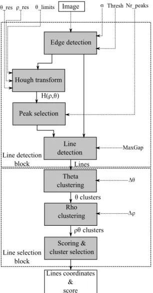
In this section,, we describe our proposed algorithm. As previously discussed we aim at providing a robust and fast railway detection method that can be used on board UAVs for tracking and orientation purposes during infrastructure surveillance. In order to achieve this we use a sequential algorithm where each block’s output is the input of the next. The whole algorithm can also be divided into two larger blocks: a line detection block and a line selection one.
In Figure 1, we depict the general scheme of the proposed al-gorithm. Our method can be divided into 7 steps, starting from the input image and finalizing with the detected lines coordinates. The first step in the algorithm is the edge detection. There are numerous algorithms that can be used for edge detection. Some of the more
Edge detection Hough transform Peak selection Line detection Theta clustering Rho clustering Scoring & cluster selection Thresh _res _res _limits Nr_peaks
MaxGap Image Lines coordinates & score H( , ) Lines clusters clusters Line detection block Line selection block
Fig. 1. Algorithm general scheme. Dotted lines indicate input data.
popular ones, that were proven over time are: Laplace, Sobel and Canny methods [9]. Unlike the first two, Canny method is less sus-ceptible to noise and for this reason it is preferred. However, the selection of σ and Thresh parameters plays an important role and should be carefully balanced. Too much smoothing may lead to a loss of useful information, while no smoothing will lead to noise in the edge detection step.
The next step of the algorithm is the Hough Transform (HT) [10] [11]. This is a well known method for detecting straight lines in images and can work even with noisy data. Several variants of the transform exist such as those described by Leavers in [12] or [13]. Fernandes and Oliveira propose in [14] a real time implementation for HT through an improved voting scheme. Frame rates of up to 52.63 are reported.
The next two steps in the our pipeline identify the lines in the image. Firstly, a selection of peaks is performed in the transform space and then lines are identified for each of the pairs of (ρ, θ). The MaxGap parameter is used to set the maximum accepted discontinu-ity, in the binary edge image, when identifying a line. Once a set of lines is identified with corresponding start/end points and associated (ρ, θ) pairs, the list is passed to the next block which performs the
line selection that best characterizes a railroad in the given context (UAV infrastructure surveillance).
The second part of our method is comprised of three blocks. Two clustering blocks for θ and ρ and a scoring and cluster selection block. In what follows we will describe each block in detail and discuss the particularities and issues that can be encountered.
A first thing to notice is that the clustering is performed in two steps as opposed to running a clustering algorithm, for all (ρ, θ) pairs, such as k-means [15]. The reason behind this is that each of the two parameters is bound by a specific condition. Performing this analysis separately allows us to identify the clusters efficiently by searching for a maximum with respect to the frequency of lines at each θ and ρ interval.
In the case of θ we know that railroads are parallel so lines be-longing to a railroad should have the same angle. Of course, due to the nature of the HT, several concurrent lines can be identified for each rail instead of two parallel lines for each rail. This is due to peaks in the HT transform that are not always isolated. These effects are caused by the quality of the image, the precision of the edge de-tection method or simply by the resolution with which the HT was computed. Therefore, a small variation should be allowed for lines that belong to a railroad. This is denoted in Figure 1 by ∆θ. Iden-tifying the θ line clusters is now simply a matter of searching for θ intervals with a high frequency of lines in a histogram computed over a quantization of the θ search domain (θlimits). The minimum quantization step in this case is given by θresand the maximum step should not be higher than ∆θ. Once a cluster is identified the lines are suppressed and the procedure is repeated. The number of clus-ters should be limited manually and also automatically in order to avoid relatively small clusters with respect to the frequency of the peak intervals. A good form for this threshold is:
F (θCk min, θ Ck max) > τ · F (θ C1 min, θ C1 max) (1) where, (θCk min, θ Ck
max) is the θ interval of the cluster, F returns the number of lines in the interval, C1is the first identified cluster which has the highest line frequency and τ is a constant between 0 and 1.
Once a set of θ clusters is identified we can proceed to separat-ing each one into multiple clusters with respect to ρ. The procedure is similar to the θ case and differs in the selection of ∆ρ. As rails are equally spaced, ∆ρ can be empirically determined for a given scenario or estimated using the drone camera parameters and alti-tude. In a similar manner with θ clustering, a stop criterion can be expressed as: F (ρCk min, ρ Ck max) > τ · F (ρ C1 min, ρ C1 max) (2) The final step of the pipeline is an analysis of the clusters and a selection of the best matching ones. The first thing required is to define what makes a cluster of lines most likely to belong to a railroad. For this purpose we propose computing a score for each cluster depending on the length of the lines and the variation of θ and ρ within each one. We will separate this score into three intermediary scores: Sθ, Sρand Sll(line lengths).
The first score Sθshould indicate the similarity of the lines an-gles within the cluster and also take into account the number of lines within the cluster. Even though, the angles are limited to an inter-val less variation should indicate a better match. Let us consider the following formulation for a single line θ score:
sCk θ (j) = ∆θ + N P i=1 |θCk(i) − θCk(j)| N (3)
where, k denotes the cluster, N is the total number of lines within the cluster and || is the absolute value. ∆θ assures a non-zero score. This is an indication of how similar the angles are within the cluster (high value indicates increased angle variation). The Sθ score for cluster Ckcan now be expressed as:
SCk θ = v u u u u u u t N · N P i=1 llCk(i) N P i=1 sCk θ (i) · llCk(i) (4)
where, llCk(i) is the length of the line i in cluster Ck. This value
can be interpreted as the geometric mean between the number of lines and the inverse of the sCk
θ weighted average with the length of the lines. Longer lines should be given more weight and a high number of lines increase the reliability of the detection.
A similar set of operations can be performed for ρ values in order to obtain SCk
ρ . Similarly to θ the lines should be relatively close to each other. We can define sCk
ρ (j): sCk ρ (j) = ∆ρ + N P i=1 |ρCk(i) − ρCk(j)| N (5) and SCk ρ : SCk ρ = v u u u u u u t N · N P i=1 llCk(i) N P i=1 sCk ρ (i) · llCk(i) (6)
The final component of the score should reflect the lengths of the lines in each cluster. Considering that all clusters contain a high number of small lines (this aspect will be further discussed in the experimental section) we are interested in evaluating only the longer lines as they will provide more information about the structure of the rail. We first select all lines with a length higher than the average line length of the cluster as:
L(llCk) = {i|llCk(i) > mean(llCk)} (7)
The line length score SCk
ll can be defined as:
SCk ll = v u u t P i∈L(llCk) llCk(i) M · N (8)
where M is the number of elements in L(llCk). Finally, score can
be written as the geometric average of SCk
ll , S Ck ρ and S Ck θ . S =q3 SCk θ · S Ck ρ · S Ck ll (9)
The cluster with the highest score is then selected as the railroad.
3. EXPERIMENTAL RESULTS
In this section we present our experimental results and discuss the methodology of the tests and the selection of parameters.
3.1. Testing data
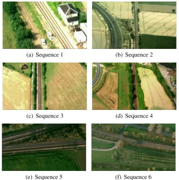
As no benchmarks and video databases currently exist for our par-ticular scenario, we use a set of video sequences acquired by Air-bus Defence & Space in the framework of the SURICATE project. The video sequences were acquired in raw YUV format and con-tain recordings of railroads located in France, captured with large, high altitude, enduring UAVs. We extracted several sequences from the drone recordings, from various locations, with different content including roads or other geometrical structures similar to railroads. Each sequence has 300 frames and a resolution of 1920 × 1080.
(a) Sequence 1 (b) Sequence 2
(c) Sequence 3 (d) Sequence 4
(e) Sequence 5 (f) Sequence 6
Fig. 2. Test sequences representative frames. Each frame shows the type of content present in each of the test sequences.
3.2. Testing Methodology
For testing purposes, we implement our algorithm in Matlab. How-ever, in the future an on-board implementation will be done in order to perform real time testing and calibration of parameters. The de-tection algorithm is applied on each frame. We consider the line detected if the line cluster is located over the railroad and has the correct angle. If the railroad is not entirely detected (e.g. the de-tected lines cover only a part of the railroad) we consider this case also as a positive detection, as having the θ and ρ intervals will pro-vide a good indication of the railroad position and relative angle to the drone. All other cases when the detected lines fail to indicate the proper angle of the rail or are located over different structures in the image are considered false detections. In addition, we will show a step by step run of the algorithm and the intermediary results. 3.3. Parameter calibration
In our tests, we used the same parameters for all test sequences. Al-though, in the future an automatic calibration is preferred, as some of the parameters are strongly linked with the drone’s camera and flight path. A large increase in speed can be obtained by reducing the search domain for θ. In normal conditions the UAV will have a predefined flight path in close proximity to the railroad. The relative angle of the railroad can be determined with respect to the aircraft by
using the GPS and geographical information. This information can be used to drastically reduce the search angle limits (θlimits) and increase the speed and reliability of the detection. However, in our experiments we used the maximum angle span from -90 to 90 de-grees, relative to the image x-axis. The HT resolution for θ and ρ is also dependent on the zoom. Once the railroad is identified the cam-era may be zoomed in and our algorithm will indicate the relative position of the railroad in the image which can be used for tracking. The resolution in this case may be lowered as the railroad will have a larger size relative to the image size. Also, based on the degree of zoom in, camera parameters and drone altitude the ∆ρ can be easily computed as railroads have constant widths. In Table 1 we report the parameters used in our tests.
Parameter value Parameter value
θres 0.4 ∆θ 3
ρres 1 ∆ρ 50
θlimits [-90, 89.6] σ 1.4 Nr peaks 150 Thresh 0.15 Table 1. Algorithm parameters used in our tests.
3.4. Results
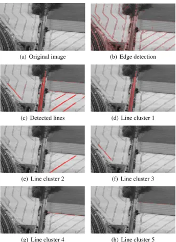
In Table 2, we report our detection rate. As can be seen we obtain a very good detection rate for the railroads. In Figure 3, we depict an
Sequence Det. rate(%) Sequence Det. rate( %) Seq. 1 99.6 Seq. 4 72,6 Seq. 2 96.6 Seq. 5 96.3 Seq. 3 94.3 Seq. 6 100 Table 2. Algorithm parameters used in our tests.
example of the algorithm’s behavior for frame 40 of Sequence 2. The detected clusters of lines are depicted, as well as the edge detection step. In Figure 3(c) we show all the detected lines. The reported score (S) for the 5 clusters is: 9.0932, 5.9146, 5.9701, 4.6062 and 3.6431. As expected the first cluster which also contains the railroad has the highest score and is selected as the detected railroad.
4. CONCLUSIONS
In this paper we presented a railroad detection algorithm for surveil-lance of infrastructure using large, high altitude, enduring drones. The method can be used for railroad tracking with the UAV’s camera and also for navigational purposes in the case of GPS or connection failure with the drone. We tested the proposed technique using a set of sequences supplied by Airbus, Defense & Space, acquired in the context of the SURICATE project which proposes infrastructure surveillance using UAVs. We were able to obtain a detection rate of 93.23 in average over all tested sequences. The algorithm was not yet integrated with the drone’s on-board systems, however, this is a future work direction. Furthermore, additional improvements can be made by creating a parameter adjustment system with respect to the drone camera and flight information data. Further improvements can be made by taking into account the temporal aspect and estimating the position of the railroad in future frames thus eliminating possible erroneous detections.
(a) Original image (b) Edge detection
(c) Detected lines (d) Line cluster 1
(e) Line cluster 2 (f) Line cluster 3
(g) Line cluster 4 (h) Line cluster 5
Fig. 3. An example of the detected lines and clustering process for frame 40 of Sequence 2. Red indicates the detected lines in the image for Figures 3(c)to 3(h). Figure 3(b) shows the detected edges with.
−100 −80 −60 −40 −20 0 20 40 60 80 −500 0 500 1000 1500
2000 Scatter plot of the detected lines in Rho/Theta space.
Theta (Deg)
Rho (pix)
(a) Line scatter plot in Rho/Theta space −1000 −50 0 50 100 50 100 150 Theta (Deg) Number of lines (b) Theta histogram −2500 −2000 −1500 −1000 −5000 0 5001000150020002500 50 100 150 Rho (Pixels) Number of lines (c) Rho histogram
Fig. 4. The line scatter plot in Rho/Theta space 4(a) and the lines histograms with respect to Theta 4(b) and Rho 4(c).
5. ACKNOWLEDGMENTS
The authors would like to thank Airbus Defense & Space for provid-ing the test sequences used in our experiments.
6. REFERENCES
[1] Radu Stoica, Xavier Descombes, and Josiane Zerubia, “A gibbs point process for road extraction from remotely sensed images,” International Journal of Computer Vision, vol. 57, pp. 121–136, 2004.
[2] Zhu Teng, Feng Liu, and Baopeng Zhang, “Visual railway detection by superpixel based intracellular decisions,” Multi-media Tools and Applications, vol. 75, no. 5, pp. 2473–2486, March 2016.
[3] Dalal N and Triggs B, “Histograms of oriented gradients for human detection,” IEEE Conf. on Computer Vision and Pattern Recognition (CVPR), pp. 886–893, 2005.
[4] David G. Lowe, “Object recognition from local scale-invariant features,” in Proceedings of the International Conference on Computer Vision, 1999, pp. 1150–1157.
[5] Fulkerson B, Vedaldi A, and Soatto S, “Localizing objects with smart dictionaries,” in Proceedings of the European Confer-ence on Computer Vision, 2008, pp. 179–192.
[6] Felzenszwalb PF, Girshick RB, McAllester D, and Ramanan D, “Object detection with discriminatively trained part-based models,” IEEE Trans Pattern Anal Machine Intell, vol. 32, pp. 1627–1645, 2010.
[7] Elod Pali, Koppany Mathe, Levente Tamas, and Lucian Bu-soniu, “Railway track following with the ar.drone using van-ishing point detection,” in IEEE International Conference on Automation, Quality and Testing, Robotics, May 2014, pp. 1–6. [8] N. Kiryat, Y. Eldar, and A. M. Bruckstein, “A probabilistic hough transform,” Pattern recognition, vol. 24, no. 4, pp. 303– 316, 1991.
[9] S. Saluja, A. K. Singh, and S. Agrawal, “A study of edge-detection methods,” International Journal of Advanced Re-search in Computer and Communication Engineering, vol. 2, pp. 994–999, 2013.
[10] P.V.C. Hough, “Methods and means for recognizing complex patterns,” 1962.
[11] R.O. Duda and P.E. Hart, “Use of the hough transformation to detect lines and curves in pictures,” Commun. ACM, vol. 15, pp. 11–15, 1972.
[12] V.F. Leavers, “Survey: which hough transform?,” Graphical Model Image Process, vol. 58, pp. 250–264, 1993.
[13] N. Kiryati, Y. Eldar, and A. M. Bruckstein, “A probabilistic hough transform,” Pattern recognition, vol. 24, no. 4, pp. 303– 316, 1991.
[14] Leandro A.F Fernandes and Manuel M. Oliveira, “Real-time line detection through an improved hough transform voting scheme,” Pattern Recognition, vol. 41, pp. 299–314, Septem-ber 2008.
[15] T. Kanungo, D. M. Mount, N. S. Netanyahu, C. D. Piatko, R. Silverman, and A. Y Wu, “An efficient k-means clustering algorithm: Analysis and implementation,” IEEE Trans. Pat-tern Analysis and Machine Intelligence, vol. 24, pp. 881–892, 2002.