GPR, ERT and CPT data integration for high resolution aquifer modelling.

(1)

GPR, ERT and CPT data integration for high

resolution aquifer modeling

Christine Bélanger

Institut National de la Recherche Scientifique Québec, Canada

Christine_Bélanger@ete.inrs.ca

Bernard Giroux

Erwan Gloaguen

Erwan_Gloaguen@ete.inrs.ca

René Lefebvre

Abstract—It is widely accepted that an integrated characterization approach is necessary to define the geometry, internal structure, material distribution and water composition of aquifers. Multiple geophysical and hydrogeological data were measured in the sub-watershed surrounding a former unlined landfill: hydrogeological data in 25 direct push full-screen wells (slug tests, water conductivity, water levels), 21 km of GPR, 5 km of 2D electrical tomography and 30 cone penetration tests (CPT) with soil moisture resistivity (SMR). The 3D data integration in gOcad facilitates data interpretation and provides the basis for a detailed numerical groundwater flow and transport models.

Keywords-component; GPR; CPT; ERT; geostatistics I. INTRODUCTION

The shallow subsurface of the earth is an extremely important geological zone as it yields much of our water resources, supports our agriculture and ecosystems, and influences our climate. Unfortunately, this zone also serves as the repository for most of our municipal, industrial and governmental wastes. Effective management and protection of natural resources is a multifaceted major societal challenge: contaminants associated with industrial, agricultural, and defense activities in developed countries; the increasing use of chemicals related to the technological development of emerging countries; the need to provide sustainable water resources for growing populations; the threat of climate change and anthropogenic effects on ecosystems. Solution to all of these questions requires the urgent improvement of our understanding of the shallow subsurface. Many agencies and councils have recently described the pressing need to develop better tools and approaches to characterize, monitor, and investigate hydrogeological parameters and processes in the shallow subsurface at relevant spatial scales and in a minimally invasive manner (e.g., [1-2]).

However, it is now well accepted that conventional groundwater characterization techniques fail to define the spatial heterogeneity of hydrogeological parameters at appropriate scales, even though this heterogeneity is the main control on contaminant transport [3]. In petroleum

studies, continuous indirect data (such as geophysical data) have proved very efficient to constrain the spatial modeling of subsurface heterogeneity based on a few sparse direct measurements [4].

In that perspective, this paper presents partial results of a project aiming to develop novel integrated subsurface characterization approaches, using geophysical and hydrogeological data, to provide a detailed definition of hydrogeological conditions, which will be the basis for a groundwater flow and transport numerical model. The application of the approach is made in a 12 km2_{area of an}

unconfined aquifer surrounding a former landfill in Saint-Lambert-de-Lauzon, 35 km southeast of Québec City (Figure 1). The sound environmental management of the landfill requires the delineation of leachate plumes migration paths and the understanding of their natural attenuation, which is controlled by physical and chemical heterogeneities affecting groundwater flow and mass transport. A high resolution characterization is thus required in order to appropriately represent aquifer conditions in the numerical model [5]. The hydrogeological dataset consists of a high resolution Digital Earth Model (DEM), hydraulic conductivity derived from multi-level slug tests and borehole flowmeter [6], multi-level geochemical fluid logging and sampling. The geophysical dataset consists in 21 km of surface GPR data, 5 km of surface electrical tomography CPTu/SMR soundings, and electrical and GPR crosshole tomography surveys [7]. The characterization program carried out in the study area leads to a large set of spatially distributed data. The first objective of the work described in this paper is to integrate these multisource data in a database with 3D geographical information system capabilities in order to facilitate their integration and their interpretation in terms of geophysical or hydrogeological conditions. Considering its accessibility, its relative ease of use and its 3D capacities, gOcad was chosen to integrate the data [8-10]. The second objective is to define the aquifer interfaces (soil topography, base of the aquifer, etc…) by geostatistically integrating GPR data and well markers [11].

(2)

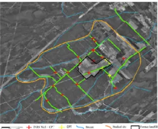
Figure 1 Location of the study area (Tremblay et al., 2008). II. STUDY AREA

The study area covers 4 km EW by 3 km NS in the municipality of Saint-Lambert-de-Lauzon, within the Beaurivage River watershed (Figure 1). The study area was delineated based on the groundwater divide between the Chaudière River watershed, to the East, and the Beaurivage River watershed, to the West, and on the hydrological physiology of the surrounding creeks. The topography is relatively flat and natural streams influence groundwater flow. Primary and secondary roads as well as forestry roads make the site easily accessible. A landfill operated by the Régie intermunicipale de gestion des déchets des Chutes-de-la-Chaudière is located in the center of the study area. In 24 years (1974 to 1997), 900 000 tones of waste from municipal, agricultural and industrial sources were buried in the former landfill of Saint-Lambert-de-Lauzon [12]. The wastes were buried above a 10-m thick sandy unconfined aquifer overlying impermeable units of clayey silt and till. The former landfill was not lined above or under the waste, which leads to leachate production due to rainfall percolation through the decomposing waste and the infiltration of this leachate in the groundwater [12]. Leachate was detected in the surrounding creeks before closure and capping of the former landfill [14]. The leachate emitted by the former landfill is presumed to naturally attenuate due to the fast and important geochemical transformations related to major changes in conditions between the leachate (highly reductive) and the aquifer (mostly oxidizing under unconfined conditions) [7]. It is to be noticed that the leachate is managed by natural attenuation. However, the efficiency of this approach has to be confirmed.

Figure 2 General context of the study area. Green lines represent the GPR surveys, red crosses represent the wells and the black lines represent the landfill.

III. DATA ACQUISITION AND ANALYSIS A. Surface ground penetrating radar (GPR)

About 21 km of GPR surveys were recorded in the study area (Green lines in Figure 2). 100 Mhz antennas were selected because they offer the best compromise between resolution and investigation depth for this area. GPR data processing consisted in 1) a dewow, 2) a static correction, 3) manual gain, 4) bandpass filtering and 5) background removal. Gain functions were adapted to each profile in order to get the best image (as judged by the user), but the gain was kept constant for all traces belonging to a given profile in order to map the attenuation. Most of the GPR profiles recorded in the study area (Figure 3) allow characterizing the stratigraphy of the aquifer to a depth of 14 meters. When bedrock is not too deep and attenuation is low, it is possible to pick the reflector representing aquifer-bedrock interface (Figure 3). This reflector exhibits important topographic variations that could not have been captured by point data from drilling or other vertical sounding methods, such as CPT. It is to be noticed that GPR data were measured before any drilling. In order to minimize the number of wells and to maximize the information, the well locations were decided based on the GPR images. The strategy consists in sampling zones showing variability in terms of the geometry of the reflection or in terms of GPR attenuation. GPR profiles often showed highly attenuated zones (e.g. left and right of Figure 3B). These attenuation zones are quite relevant, as they were found to correspond to variations in groundwater conductivity related to changes in total concentrations of dissolved solids. This induces higher bulk conductivity that attenuates the GPR signal. In many instances, these attenuated zones represent regions where landfill leachate is found [7].

(3)

A)

B)

Figure 3. Two typical GPR profiles. The reflector highlighted in blue represent till or the top of bedrock, which corresponds to the unconfined aquifer base.

B. Surface 2D electrical tomography

A total of 5 km of resistivity profiles was recorded in the study area. The resistivity profile location was selected on the basis of GPR and CPT soundings and the hydrogeological context. The inversion of the data was carried out using Res2dinv (Geotomo Software). To honor topography, which influences inversion results, each electrical survey line was imported in ArcGIS where their

coordinates and relative elevation were extracted from the high resolution DEM. The chosen inversion algorithm used a standard constraint with five iterations. The damping factor was kept constant because tests showed that it did not sensibly improve the RMS error. Furthermore, numerous inversions parameters were tested to validate the final image and confirm that the resulting resistivity profile was mainly supported by the data and not by the inversion parameters.

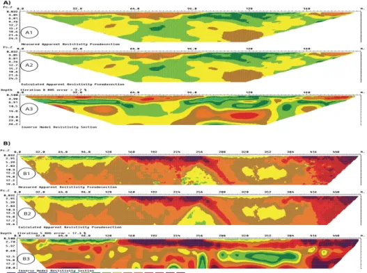
Figure 4A shows a resistivity profile measured directly down gradient of the former landfill site. The processed resistivity image (Figure 4 A3) shows low resistivity associated to low resistivity water typical for contaminated water. Figure 4B shows a resistivity profile measured up gradient of the landfill at the same location than the GPR profile shown in Figure 3B. The resistivity image shows low resistivity contrasts compared to Figure 4A, indicating less contaminated water. Furthermore, the profile seems to confirm the low resistivity zone at 290-390 m location and suggest that the strong attenuation in the GPR profile in Figure 3B is caused by changes in ground electrical property in depth. Well installations allowed the measurement of groundwater conductivity and confirmed that the resistivity zones were due to a decrease in water resistivity

Figure 4 A) Electrical survey over the landfill. B) Electrical survey outside the landfill (same location as GPR profile in Figure 3B). A1: measured apparent resistivity; A2: computed apparent resistivity leading to A3; A3: inversed "true" resistivity. B1: measured apparent resistivity; B2: computed apparent resistivity leading to B3; B3: inversed “true” model.

C. Cone penetration tests (CPT) with soil moisture resistivity (SMR)

CPT/SMR soundings measure mechanical (CPT) and electrical/dielectric (SMR) properties of unconsolidated

competent layer). CPT/SMR data can be correlated to soil properties and material types [15]. In the study area, CPT/SMR soundings were carried out with a versatile and mobile Geotech 605D track-mounted geotechnical drilling rig. Measured parameters were tip stress, sleeve stress, pore pressure, global resistivity and water content (or

(4)

rig, a direct push technique efficiently allows the installation of full-screen monitoring wells. This well installation technique does not require a sand pack between the aquifer material and the screen.

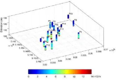
Figure 5 Spatial distribution of CPT soundings over the studied area.

More than 30 CPT/SMR soundings were carried out in the study area, with locations based initially on prior surface GPR surveys and lately on the combination of surface GPR and electrical tomography. The surface geophysical surveys provide information on variations of aquifer conditions, thus allowing the selection of CPT/SMR soundings in a priori known hydrogeological contexts. Hence, CPT soundings were mainly done in areas showing strong physical property contrasts. Figure 5 shows the location of bulk resistivity profiles obtained from 16 CPT/SMR soundings. This figure demonstrates a clear increase in the electrical conductivity from well P14 (up gradient from the landfill) to P12 in the lower left part. This high resistivity zones suggests the extent of leachate emitted from the former landfill.

IV. INTERPOLATION OF AQUIFER BOUNDARIES An initial step of the assessment of hydrogeological conditions consists in defining the main aquifer boundaries, which for our study area are the soil surface, the water table and the base of the aquifer. In absence of indirect data, those interfaces are usually defined on the basis of limited direct data, thus often requiring arbitrary user control. Given the high variability of the aquifer base shown on GPR surveys, such a conventional approach could not capture the variability of this surface. In that context, and given the large amount of available indirect data, a geostatistical approach was selected to follow techniques developed in the petroleum industry, where few wells are available but extensive indirect measurements are [17].

Interpolation of topographic surface: First, the topography of the ground surface elevation is interpolated. The adopted methodology was to cokrige the measured high precision but scarce GPS elevation points and a

publicly available Digital Elevation Model (DEM). Collocated cokriging was retained as it is numerically efficient and stable when the secondary data are oversampled like DEM data [18- 19]. Also, collocated cokriging only requires the modeling of the secondary data variogram [4]. This interpolation strategy allows optimal integration of the continuous but not precise DEM elevations and the high precision but sparse GPS elevations.

Interpolation of water table surface: Over a century ago, [20] recognized the close relationship between the water table and topography and suggested that topography should be used to constrain the water table elevation. In order to fill the sparse water level data measured at wells, many studies proposed to use the topography as indirect data. The incorporation of indirect data can be done through deterministic or probabilistic ways. [21] appear to be the first to integrate topography with groundwater levels measurements in wells for the geostatistical estimation of the potentiometric surface. Many authors [21-22] have estimated the water-table surface with ordinary cokriging using water elevations as primary variable and ground surface elevations as secondary variable. These studies all show the same outcome, i.e. the water table cokriging estimation is more accurate than one made only with ordinary kriging if the secondary variable (ground surface elevation) is available at all measured points of the primary variable (groundwater level). Recent papers show implementation of the KED either by using linear function between water-table depth and DEM-derived quantity known as topographic index [19] or by incorporating linear model of coregionalization and Markov models [23].

Interpolation of the aquifer base surface: Similarly to the previous surfaces, the aquifer thickness was cokriged using depth to bedrock and GPR picked travel times at the aquifer till interface (blue circles in Figure 3). Contrary to the two other surfaces, the indirect data are not available at all interpolation locations. Hence, the chosen algorithm was full cokriging. This algorithm requires the calculation and modeling of the variograms of travel times and the aquifer thickness (depth to the till layer identified at well locations) and also the cross-variogram between travel times and aquifer thickness. Once the aquifer thickness is cokriged, the interpolated thicknesses are removed from the topographic surface in order to obtain the aquifer base elevation.

V. 3D DATA INTEGRATION

The main goal of this study is to integrate all available information in order to produce the numerical flow model with the highest resolution possible. However, the large amount of multisource data makes their interpretation challenging when each data is considered separately in 2D. Furthermore, some 3D GIS allow the generation of meshgrids that are easily exportable to numerical flow simulators such as Feflow [24]. Hence, building a 3D model can be done directly in 3D, which saves time and allows a better spatial control on adjacent information when modeling. The 3D integration in gOcad is a way to

(5)

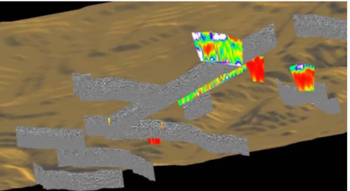
quickly visualize and interpret the data together. With all those parameters in 3D it is possible to follow important interfaces and link them to make surfaces. For example, each reflector associated to the aquifer-bedrock interface on the GPR surveys is flagged to the measured depth on CPT. Combination of both data into geostatistical analysis allow the computation of high resolution bedrock topography. Also, 3D visualization better displays the 3D behavior of the very complex stratigraphy. In addition, the 3D visualization allows the comparison and validation of the different data types. For example, Figure 6 shows the GPR profile in Figure 3B and the resistivity profile in Figure 4B. This integration confirms that GPR attenuation is due to a decrease of the aquifer bulk resistivity (red zone on the right). Also, the strong reflections near the surface are associated to low resistive pools (in red) that are typical for peat zone in the study area.

Figure 6 Superposition of figures 3B and 4 in gOcad Figures 7 and 8 show different views of the available geophysical data. These data clearly shows a decrease in the electrical resistivity over the entire landfill area (red anomalies on resistivity profiles). Also, the GPR data analysis shows promising potential to identify the different boundaries and internal structure of the different lithofacies. For example, the sand layer seems to be interdigitated with discontinuous silty-sand layers. Also, the GPR profiles allow identifying a superficial clay layer which will have a great importance in the flow model. In addition, CPT data (Figures 7 and 8) help differentiating the changes in lithologies from the changes in electrical groundwater conductivity, as mechanical data are not sensitive to changes in groundwater conditions.

Figure 7 Global view of the integration in gOcad (perspective view)

Figure 8 Global view of the integration in gOcad (near horizontal view)

VI. CONCLUSION

An integrated characterization approach was developed to define the geometry, internal structure, material distribution and water composition of an unconfined aquifer in the sub-watershed surrounding a former unlined landfill. Multiple geophysical and hydrogeological data were acquired for that purpose, each type of data providing different types of complementary information to characterize the leachate plume and define the aquifer thickness variability and material heterogeneity. One of the first insights of the study was that simply bringing all those information together in a same 3

D GIS improves the

communication between the different people coming from different disciplines. This results in a more effective understanding of the aquifer structure and of the leachate spatial distribution.

Interesting initial result include a lower global resistivity near the former landfill site, which increases as the distance from the landfill increases, thus providing indications of leachate extent and migration paths. GPR profiles have attenuation areas, which also correlate with a decrease in water resistivity. CPT logs help identifying the different reflectors in GPR profiles and the type of materials. The bedrock contact, aquifer surface and topography were adjusted and integrated in the 3D model. With the different data, it will be possible to link the diverse structures of the lithology so as between the leachate plume. All those data will allow the understanding of a complex system by extracting the maximum of information from the gathered data. This understanding will support the development of a detailed and representative numerical model of groundwater flow and mass transport.

ACKNOWLEDGEMENTS

This study was supported by the Régie intermunicipale de gestion des déchets des Chutes-de-la-Chaudière and by NSERC Discovery Grants held by E.G. and R.L.

REFERENCES

[1] Ministère du Développement durable, de l’Environnement et des Parcs (MDDEP), 2008. Programme d’acquisition de connaissances sur les eaux souterraines du Québec – Guide des conditions générales. ISBN 978-2-550-53934-6 (pdf).

[2] Council of Canadian Academies, 2009. The Sustainable Management of Groundwater in Canada. CCA, The Expert Panel on Groundwater, Ottawa, ISBN 978-1-926558-11-0.

(6)

[3] Marsily, Gh. de, Delay, F., Gonçavès, J., Renard, Ph., Teles, V., Violette, S. 2005. Dealing with spatial heterogeneity. Hydrogeology Journal, 13, 161-183.

[4] Goovaerts, P. 1997. Geostatistics for natural resources evaluation. Oxford University Press, New York, Oxford.

[5] Paradis, D., Gloaguen, E., Lefebvre, R., Tremblay, L., Ballard, J-M. Morin, R. 2008. Multivariate integration of CPTu/SMR and hydraulic conductivity measurements for the definition of hydrofacies in unconsolidated sediments. GeoEdmonton ‘08, Edmonton, Canada, Paper 224, 1470-1477.

[6] Paradis, D., Lefebvre, R., Morin, R., Gloaguen, E. 2009. Using borehole flowmeter data to optimize hydraulic conductivity characterization in heterogeneous unconsolidated aquifers. GeoHalifax ‘09, Halifax, Sept. 20-24, 2009.

[7] Tremblay, L., Gloaguen, E., Lefebvre, R., Ballard, J-M., Paradis, D., Michaud, Y. 2008. Integration of geophysical, geochemical, and direct push methods for the detection of leachate plumes. GeoEdmonton ‘08, Edmonton, Canada, Paper 175, 1142-1146 [8] Earth Decision Sciences 2001. GOCAD 2.0 user’s manual. 1 564

pp.

[9] Mallet J.-L. 1992. gOcad: A computer-aided design program for geological applications. In: Turner K (ed) Three-dimensional modeling with Geoscientific Information Systems, Kluwer Academic Publishers, Dordrecht, Holland, Nato ASI Series C, 354:123–141

[10] Mallet J.-L. 2002. Geomodeling. In: Journel A.G. (ed) Applied geostatistics series, Oxford University Press, Oxford.

[11] Routin, G., Gloaguen, E., Lefebvre, R. 2008. Modélisation de l'enveloppe d'un aquifère, par approche géostatistique. GeoEdmonton ‘08, Edmonton, Canada, Paper 229, 1507-1514. [12] Régie intermunicipale de gestion des déchets des

Chutes-de-la-Chaudière 2006. Internet site www.chaudiere.com/regiedechets/

[13] Fetter, C.W. 2001. Applied hydrogeology (4th_{Ed.). Prentice Hall,}

118-120.

[14] Géoroche Ltée, 1985. Étude hydrogéologique-Lots P-258 à P-265 St-Lambert de Lauzon. N/D 5125-0000-0000

[15] Fauveau, É., Lefebvre, R., Ballard, J.-M., Fortier, R., Martel, R. 2005. Examples of hydrogeological characterization of unconsolidated sediments with direct push and rotopercussion technologies. 58th_{Canadian Geotechnical Conference and 6}th_Joint

CGS/IAH Conference, Saskatoon, Canada, October 2005, Session 11EA, Paper 565, 8 pp.

[16] Ouellon, T., Lefebvre, R., Marcotte, D., Boutin, A., Blais, V., Parent, M. 2008. Hydraulic conductivity heterogeneity of a local deltaic aquifer system from the kriged 3D distribution of hydrofacies from borehole logs, Valcatier, Canada. J. of Hydrology, 351 (1-2), 71-86.

[17] Chilès, J. P., Delfiner, P., 1999. Geostatistics: Modeling spatial uncertainties. New York, Wiley-Interscience.

[18] Comeau, G., Gloaguen, E., Nastev, M., Martel, R. 2009. Improvment of water table estimation using multiple direct and indirect data in collocated cokriging at the Canadian Forces Base of Petawawa, Ontario. Submitted

[19] Desbarats, A.J., Logan, C.E., Hinton, M.J., Sharpe, D.R. 2002. On the kriging of water table elevations using collateral information from a digital elevation model. Journal of Hydrology, 255, 25-38. [20] King, F.H. 1899. Principles and conditions of the movements of

groundwater. US Geological Survey

[21] Hoeksema, R.J., Clapp, R.B., Tomas, A.L., Hunley, A.E., Farrow, N.D., Dearstone, K.C. 1989. Cokriging model for estimation of water table elevation. Water Resources Research, 25, 429-438. [22] Deutsch, C.V., Journel, A.G. 1992. GSLIB Geostatistical software

librairy and user's guide. Oxford University Press, New York. [23] Boezio, M., Costa, J., Koppe, J., 2006. Accounting for Extensive

Secondary Information to Improve Watertable Mapping. Natural Resources Research, 15, 33-48.

[24] Diersch, H.J.G. 2004. FEFLOW: Finite Element Subsurface Flow and Transport Simulation System – Reference Manual. WASY Institute. 27