CIRPÉE
Centre interuniversitaire sur le risque, les politiques économiques et l’emploi
Cahier de recherche/Working Paper 05-16
Collective Labor Supply: a Single-Equation Model and Some
Evidence from French Data
Olivier Donni Nicolas Moreau
Mai/May 2005
_______________________
Donni: THEMA, Université de Cergy-Pontoise, 33 Boulevard du Port, 95011 Cergy Cedex, France olivier.donni@eco.u-cergy.fr
Moreau: GREMAQ and LIRHE, Université de Toulouse 1, Manufacture des Tabacs, bat. F, 21 allée de Brienne, 31000 Toulouse, France
nicolas.moreau@univ-tlse1.fr
This paper was partly written while Nicolas Moreau was visiting CIRPÉE, Université Laval, whose hospitality and financial support are gratefully acknowledged. We thank François Bourguignon for useful comments and suggestions. We bear the sole responsibility for any remaining errors.
Abstract:
In Chiappori’s (1988) collective model of labor supply hours of work are supposed flexible. In many countries, however, male labor supply does not vary much. In that case, the husband’s labor supply is no longer informative about the household decision process and individual preferences. To identify structural components of the model, additional information is needed. We thus consider an approach in which the wife’s labor supply is expressed as a function of the household demand for one specific good. We demonstrate that the main properties of Chiappori’s initial model are preserved and apply our results on French data.
Keywords: Collective Models, Labor Supply, Intra-household Distribution,
Conditional Demand
1
Introduction
The collective model of labor supply, developed by Chiappori (1988, 1992), is by now a standard tool for analyzing household decisions. This model is based on two fundamental hypotheses — each household member is characterized by speci…c preferences, and decisions result in Pareto-e¢ cient outcomes — which turn out to be su¢ cient to generate strong testable restrictions on spouses’labor supply. Moreover, if consumption is purely private and agents are egoistic, the characteristics of the structural model, such as individual preferences and the rule that determines the distribution of welfare within the household, can be identi…ed from the observation of spouses’labor supply.1
These features of the collective model have turned out to be very attractive, and the number of empirical studies based on Chiappori’s initial framework is consid-erable. These include Bloemen (2004, Netherlands), Chiappori, Fortin and Lacroix (2002, United States), Clark, Couprie and Sofer (2004, United Kingdom), Fortin and Lacroix (1997, Canada), Moreau and Donni (2002, France) and Vermeulen (2005, Belgium). However, the large majority of these investigations does not account for the fact that, in most developed countries, male labor supply is rigid and largely determined by exogenous constraints. If the dispersion in husbands’hours is very limited and/or does not stem from spouses’ optimal decisions, the identi…cation results given in Chiappori’s papers may well be inappropriate.
One important exception in the empirical studies devoted to collective models is given by Blundell et alii (2004). These authors emphasize that in the United Kingdom (but this certainly holds true in other countries), if men work, they work nearly always full-time; the wife’s working hours, on the contrary, are largely dis-persed. The theoretical model they develop then allows for these essential features: the wife’s labor supply is assumed to be continuous, whereas the husband’s choices are assumed to be discrete (either full-time working or non-working). These authors show that the main conclusions which were derived by Chiappori in the initial con-text are still valid here. One drawback, however, is that the result of identi…ability and testability given by Blundell et alii (2004) holds only if the husband’s choice
1The collective model of labor supply has recently been extended in various directions.
Chiap-pori, Blundell and Meghir (2004) allow for the existence of both private and public consumption. Donni (2003) incorporates the possibility of non-participatory decisions and non-linear taxation. Apps and Rees (1997), Chiappori (1997) and Donni (2005a) recognize the role of domestic pro-duction and allow for the fact that a proportion of non-market time is spent producing goods and services within the household. Fong and Zhang (2001) study a collective model of labor supply where there are two distinct types of leisure : one type is each person’s independent (or private) leisure, and the other type is spousal (or public) leisure. See Vermeulen (2002) and Donni (2005b) for a survey of collective models.
between full-time working and non-working is free; in particular, it could be seri-ously misleading if unemployment is mistakenly interpreted as the decision of not participating in the labor market.
In the present paper we deal with the rigidity of the husband’s behavior in the French labor market. The approach is quite di¤erent from Blundell et alii’s (2004), though. The starting observation is that the variability in the husband’s working hours is very limited. In addition, since the behavior of the few husbands who do not work can probably be explained by exogenous constraints (e.g., involuntary unemployment), the employment status of the husband can hardly give reliable information about individual preferences and the decision process. The strategy adopted in what follows is then to exploit the information in household consump-tion to derive testable restricconsump-tions and identify the intra-household distribuconsump-tion of welfare.2 More precisely, we propose a very simple approach to model wives’labor
supply, in which the wife’s behavior is explained by her wage rate, other household incomes, socio-demographic variables and the demand for one good consumed at the household level. In that case, as is explained in what follows, the level of the conditioning good summarizes the most important characteristics of the decision process. We then demonstrate that the estimation of this single-equation permits to carry out tests of collective rationality and identify some elements of the struc-tural model. In addition we also show that the present framework is compatible with home production if the production function belongs to some speci…c family of separable technologies.
This framework is advantageous at three levels. Firstly, the theoretical results do not postulate a particular explanation for the rigidity of the husband’s behav-ior. Contrary to Blundell et alii (2004), identi…cation does not exploit the quite limited variations in husbands’working hours, which may well stem from demand side constraints. Secondly, the econometric techniques developed for the estimation of single-equation models can be used to estimate the wife’s labor supply, since the determination of the demand for the conditioning good needs not to be explicitly modelled. Thirdly, the variables which a¤ect the distribution of power within the household need not to be exactly observed. They are summarized by the level of the conditioning good. This point is explained in the remainder of the paper.
These theoretical results are followed by an empirical application using French data for those couples in which the wife participates in the labor market and the husband works full-time. The conditioning good is the household expenditures on food at home. The wife’s labor supply is then estimated by GMM, taking into
2The strategy is thus analogous in some respects to that in Donni (2005c), who estimates a
account the selection bias (which results from the selection of the sample). The restrictions which are derived from Pareto e¢ ciency are tested and not rejected by the data.
The paper is structured as follows. The theoretical model is developed in Section 2 and a very general functional form is presented in Section 3. The data and the empirical results are described in Section 4. All the proofs are collected in Appendix A.
2
Theory
2.1
Basic framework
Preferences and budget set. We consider only the case of a two-person house-hold, consisting of a wife (f ) and a husband (m), who make decisions about leisure and consumption.3 The market labor supply of spouse i (i = m; f ) is denoted by h
i,
with market wage rate wi. The private consumption can be broken down into two
aggregate goods, which are denoted by ci and xi, so that each household member
is characterized by speci…c preferences over (hi; ci; xi). These can be represented by
utility functions of the form:
ui(T hi; ci; xi; z); (1)
where T is total time endowment and z is a vector of socio-demographic factors,4
that are both strongly concave, in…nitely di¤erentiable and strictly increasing in (T hi), ci and xi. The household members are said to be ‘egoistic’ in the sense
that their utility only depends on their own consumption and leisure. This may seem restrictive but, as shown in Chiappori (1992), all the results immediately extend to the case of ‘altruistic’agents in a Beckerian sense with utilities represented by the form:
Wi[um(T hm; cm; xm; z); uf(T hf; cf; xf; z)],
where Wi( )is a strictly increasing function. The crucial hypothesis is the existence
of some type of separability in the spouses’preferences.
At this stage, we suppose that there is no domestic production.5 Let y be the household non-labor income. The budget set is then written as:
y + hmwm+ hfwf > c + x (2) 3The couple is not necessarily married. The terminology is chosen for convenience.
4For convenience we suppose that the same socio-demographic factors z enter both utility
functions.
5This assumption is relaxed in Section 2.5. We shall show that our theoretical results continue
and
06 hi 6 T; ci > 0; xi > 0. (3)
where c = cm+ cf and x = xm+ xf. We may note that, in consumer expenditure
surveys, consumption is usually recorded at the household level. We thus assume in what follows that the econometrician observes hi, c and x, but does not observe ci
and xi.
In France — and in many other countries for that matter — the distribution of the number of men’s working hours is very concentrated around the full-time bound. Consequently, as a convenient approximation at least, we assume the husband’s labor supply is constant, i.e.,
hm = h ; (4)
where 0 < h 6 T. The reason for this rigidity is beyond the scope of this paper. It may result from the husband’s preferences, demand-side constraints or institutional rigidities. Quite importantly, however, our theoretical results are general in the sense that they do not rely on a speci…c explanation of the husband’s behavior.
Pareto e¢ ciency and optimization. The main originality of the e¢ ciency ap-proach is the fact that the household decisions result in Pareto-e¢ cient outcomes and that no additional assumption is made about the process. That means, for any wage-income bundle, the labor-consumption bundle chosen by the household is such that no other bundle in the budget set could leave both members better o¤. This assumption, even if not formally justi…ed, has a good deal of intuitive appeal. First of all, the household is one of the preeminent examples of a repeated game. Then, given the symmetry of information, it is plausible that agents …nd mechanisms to support e¢ cient outcomes since cooperation often emerges as a long-term equilib-rium of repeated noncooperative relations. A second point is that axiomatic models of bargaining with symmetric information, such as Nash or Kalai-Smorodinsky bar-gaining, which have been previously used to analyze negotiation within the house-hold (Manser and Brown, 1980, and McElroy and Horney, 1981), assume e¢ cient outcomes.
Taking account of the restriction on the husband’s working hours, Pareto-e¢ ciency essentially means that a scalar exists so that the household behavior is a solution to the following program:
max
fhi;ci;xiji=m;f g
(1 ) uf(T hf; cf; xf; z) + um(T hm; cm; xm; z) (5)
with respect to (2)–(4). The parameter has an obvious interpretation as a ‘distrib-ution of power’index. If = 0, the household behaves as though the wife always got
her way, whereas, if = 1; it behaves as if the husband was the e¤ective dictator. To obtain well-behaved labor supplies and demands, however, we assume that is a single-valued and in…nitely di¤erentiable function of wf, wm, y and z, with a range
comprised between 0 and 1. This is standard in the literature on collective models.
2.2
Decentralization and functional structure
Let us de…ne = y + h wm as the ‘nonwife’income. As is well-known (Chiappori,
1992), if agents are egoistic and consumption is purely private, Pareto e¢ ciency implies that the household decision process can be decentralized. More precisely, if (hm; hf; cm; cf; xm; xf)are solutions to Program (5), a sharing ( ; ) of nonwife
income exists so that the husband’s and the wife’s behaviors can be described by the following programs:
A. Husband’s Program: max cm;xm um(T h ; cm; xm; z) subject to cm+ xm 6 , cm > 0 and xm > 0; B. Wife’s Program: max hf;cf;xf uf(T hf; cf; xf; z) subject to cf + xf = + hfwf, 06 hf 6 T, cf > 0 and xf > 0:
In general, the sharing of will depend on wf, wm, y and z. Hence, without loss of
generality, we write the husband’s share as: = (wf; ; s; z), where s = y= is the
ratio of nonlabor income and nonwife income. In standard terminology the variable s is called a distribution factor. In what follows, the husband’s share ; expressed as a function of (wf; ; s; z); is referred to as the sharing rule.
The result above determines the functional structure that characterizes the wife’s labor supply and the household’s demand for goods. Let us denote the solutions to the wife’s and husband’s optimization programs (in terms of what is observable) by c(wf; ; s; z), x(wf; ; s; z)and hf(wf; ; s; z). Then we have:
x(wf; ; s; z) = m( (wf; ; s; z); z) + f(wf; (wf; ; s; z); z), (6)
where m and f are the husband’s and wife’s Marshallian demand for good x
respectively, and
where f is the wife’s Marshallian labor supply. In particular, this relation satis…es Slutsky Positivity : @ f @wf @ f @( ) hf > 0 (8) for an interior solution. Note that the husband’s wage rate in‡uences the husband’s behavior only through the individual shares of nonwife income. In particular the function m is independent of wm (conditionally on ). This property is a direct
consequence of the husband’s labor supply rigidity.
2.3
The s-conditional approach
In the present section we de…ne a speci…c concept of conditional labor supply whereby the labor supply is expressed as a function of various variables and the level of good x. Note that conditional demands or supplies are often used in tradi-tional analysis where a single utility function is assumed.6 However, the conditional
function concerned here is somewhat di¤erent. First, let us assume that:
@x
@s 6= 0 (9)
in an open subset of the domain of x(wf; ; s; z), i.e., the source of nonwife
in-come (locally) in‡uences the demand for good x. Then, from the implicit function theorem, the demand for good x can be inverted on s to yield s = s(wf; ; x; z).
Let us incorporate this into the wife’s share of income and obtain what we call the ‘s-conditional’sharing rule, denoted by
(wf; ; x; z) = (wf; ; s(wf; ; x; z); z):
The s-conditional sharing rule has a speci…c property that is described in the fol-lowing lemma.
Lemma 1 The s-conditional sharing rule is implicitly de…ned as the solution of: x = m( (wf; ; x; z); z) + f(wf; (wf; ; x; z); z).
The proof is straightforward: for any , the equation of demand for good x must be identically satis…ed. This implies that the s-conditional sharing rule has a property of separability.
6See for instance Pollak (1969), Chavas (1984), Browning and Meghir (1991) or Browning (1998).
Now let us assume that there are no corner solutions. In particular the wife participates in the labor market. We then introduce the s-conditional sharing rule into the wife’s labor supply and obtain:
hf(wf; ; x; z) = f(wf; (wf; ; x; z); z); (10)
where (wf; ; x; z) has the property given in Lemma 1. We shall refer to this
concept as the ‘s-conditional’ labor supply.7 Note that in (10) the information
concerning the source of nonwife income, represented by s, is completely summarized by the level of the conditioning good x.
There are two distinct advantages to modelling an s-conditional labor supply instead of a direct one. Indeed, in modelling an s-conditional labor supply, there is no need:
(i) to model the determination of the conditioning good explicitly.
The s-conditional approach does not require an explicit structural model for the conditioning good at all. In contrast to usual collective models of labor supply à la Chiappori (1988, 1992), the s-conditional labor supply can be esti-mated with single-equation techniques.8 This is useful because the estimation
of labor supply models is generally very expensive in computer-time. (ii) to observe the distribution of nonwife income between its sources.
This is particularly compelling since, in empirical work, such information is often unreliable. More generally, the e¤ect of any distribution factor, even unobserved or unknown for the econometrician, is incorporated in the condi-tioning good.
Nevertheless, the attractiveness of the s-conditional approach largely depends on the properties of s-conditional labor supplies, namely, whether the underlying assumptions are testable and the structural model identi…able from the observation of one s-conditional labor supply. These important questions are examined in the next section.
7This concept is not completely original, though. Bourguignon, Browning and Chiappori (1995)
examine this form of conditional functions in the context of demand analysis with constant prices. Donni (2004) considers the case of variable prices. However, these authors suppose that the conditioning good is consumed by only one person in the household, which makes things much simpler.
2.4
Properties of s-conditional labor supplies
In order to investigate the testability and identi…ability issues we assume that the wife’s s-conditional labor supply exists over an open subset S. We now introduce some pieces of notation:
(wf; ; x; z) = @hf @ @hf @x 1 ; (wf; ; x; z) = @hf @x @ @ @hf @x @ @x @hf @ 1 .
In the discussion of Proposition 2 below, we shall show that (wf; ; x; z)represents
the slope of the husband’s Marshallian demand for good x, whereas (wf; ; x; z)
corresponds to the inverse of the derivative of this slope.
Let us assume now that the wife’s s-conditional labor supply satis…es some reg-ularity conditions.
Assumption R The wife’s s-conditional labor supply is such that @hf @x 6= 0, @ @x 6= 0 and @ @ @hf @x 6= @ @x @hf @ ; for any (wf; ; x; z) 2 S.
Note that, if the wife does not participate in the labor market, these conditions do not hold, and the conclusions that follow are not valid.
The next result states that the s-conditional sharing rule can be retrieved from the sole observation of the wife’s s-conditional labor supply.
Proposition 2 Let us assume that the wife’s s-conditional labor supply hf(wf; ;
x; z) satis…es R. Then,
(a) the s-conditional sharing rule can be retrieved on S up to a function k(z) of z; speci…cally, its derivatives are given by
@ @wf = @ @wf , @ @x = @ @x , @ @ = @ @ ;
(b) for each choice of k(z), the wife’s marginal rate of substitution between total consumption (c + x) and leisure (T h), i.e., the preferences between total consumption and leisure, is uniquely de…ned;
(c) the wife’s Marshallian labor supply and the individual Marshallian demands can be retrieved up to a function of z.
The complete proof of this proposition is given in Appendix A. We brie‡y give the …rst step of the argument here. By de…nition, the slope of the husband’s Marshallian demand for good x is given by the increase in x due to a one-unity variation in , keeping , wf and z constant. Note now that hf depends only on , wf
and z. Then, a one-unity variation in ; so that hf, wf and z remain una¤ected,
provides the slope of the husband’s Marshallian demand. Consequently, if we apply the implicit function theorem to hf(wf; x; ; z) such that x is di¤erentiated with
respect to , we obtain the slope of the husband’s Marshallian demand: @ m
@ =
@hf=@
@hf=@x
= . (11)
Note that @ m=@ (and thus ) depends only on and z. The identi…cation of the s-conditional sharing rule then follows from the di¤erentiation of (11) and the resolution of the system of partial di¤erential equations that results.
The s-conditional approach has two main drawbacks as far as identi…cation issues are concerned. Firstly, even if the s-conditional sharing rule can be recovered (up to a function of z), its theoretical interpretation is unclear. The reason is that the s-conditional sharing rule is expressed as a function of the level of good x, which is endogenously determined. Secondly, the s-conditional sharing rule and the other structural elements can be retrieved as long as the wife participates in the labor market but the identi…cation cannot be extended beyond the participation set. However, these drawbacks are simply a converse of the fact that we need less information to estimate an s-conditional labor supply than a system of unconditional labor supply and demand of goods, as in Donni (2005c). In particular there is neither a need to observe the level of the demand for good x when the wife does not work, nor one to observe the sources of nonwife income.
We show in the next proposition that the wife’s s-conditional labor supply has to satisfy some constraints to be consistent with collective rationality.
Proposition 3 Let us assume that the wife’s s-conditional labor supply hf(wf;
; x; z) satis…es R. Then, for any (wf; ; x; z)2 S,
(a) @hf @wf @hf @x @ =@wf @ =@x hf (@ =@x) > 0; (b) @ @wf @ @x @ @x @ @wf = @ @ @ @x @ @x @ @ = 0.
These restrictions provide a joint test of collective rationality under speci…c as-sumptions, i.e., consumption is purely private, there is no domestic production and agents are egoistic (or caring). The inequality (a) results from condition (8) trans-posed into the s-conditional context. The system of partial di¤erential equations (b) is due to the separability property that characterizes (6) and (7). The proof of that is provided in Appendix A.
We now suppose that leisure and goods are superior (i.e., normal). In many circumstances this assumption is uncontroversial because goods are very aggregated. If so, the s-conditional approach implies several additional restrictions which are presented in the next proposition.
Proposition 4 Let us assume that the wife’s s-conditional labor supply hf(wf;
; x; z) satis…es R. Then, for any (wf; ; x; z)2 S,
(a) if leisure is superior, @hf=@x
(@ =@x) > 0;
(b) if goods x and c are superior (for both spouses),
min 1; 1 + 1 + wf(@hf=@x)
(@ =@x) > > max 0; 1
(@ =@x) .
This result, which is a straightforward consequence of Proposition 2, provides a new test of collective rationality under the additional assumption of consump-tion superiority. In particular the second statement of Proposiconsump-tion 4 deserves some comments. If one inequality in this statement is violated by , then (at least) one slope of the four Engel curves must be negative. To illustrate that, let us remember that coincides with the slope of the husband’s Engel curve for good x. Then, if < 0, good x is inferior for the husband (but good c is necessarily superior from the Engel’s aggregation condition). On the contrary, if > 1, good x is superior and good c is inferior. The interpretation of the other inequalities, which are related to the wife’s behavior, are more complicated, though. The reader is referred to the proof in Appendix A.
2.5
Another interpretation: the role of domestic production
Undoubtedly, the absence of domestic production is a serious shortcoming of the model developed above. Hence, in this subsection, we incorporate the fact that a proportion of time not allocated to market labor supply may be spent producing
goods within the household. To do so, we suppose that h1
i = hi+ h2i, where h1i and
h2
i respectively is spouse i’s total labor supply and domestic labor supply.9 That
means, non-market time can be broken down into time consumed in leisure, T h1i, and time spent in domestic production, h2i. Then we suppose that goods can be
produced using ‘individual’technologies of the form: h2i = fi(c2i; x
2
i) (12)
where fi is a function, increasing and strictly convex in its arguments, and c2i et x2i
denote the proportion of goods c and x entering spouse i’s production process, where as usual a positive number indicates an output and a negative number indicates an input. Note that goods c and x are marketable in the sense that they can either be purchased (or sold) in the market or produced at home.10 Also, the prices are
exogenously …xed by the market.
In the speci…cation of the production technology, the fact that fi does not depend
on h2
j (j 6= i) is crucial in the development that follows. That implies there is
neither substitutability nor complementarity in spouses’time inputs. Overall, this assumption seems to be supported (as a valid approximation at least) by the rare empirical studies of domestic activities (e.g., Graham and Greene, 1984). Now let us suppose that spouses’utility is a function of leisure (instead of nonmarket time) and consumption. We have:
vi(T h1i; c1i; x1i); (13)
where c1
i and x1i denote the proportion of c and x which is ‘directly’consumed by
spouse i (which includes the outputs of the production process and excludes the inputs). We have: c1
i = ci+ c2i and x1i = xi+ x2i, where ci and xi denote the quantity
of goods purchased in the market for spouse i’s use.
The basic idea of the reasoning is that if the production technology is of the form (12), the utility function (1) which is used in the preceding subsections can be derived from a more fundamental representation of preferences, described by (13). We have: ui(hi; ci; xi) = max c1 i;x1i;c2i;x2i vi(T hi fi(c2i; x 2 i); c 1 i; x 1 i); (14) subject to c1i c2i = ci; x1i x 2 i = xi:
9To simplify the presentation of this subsection and emphasize the intuition, we do not take into
account the rigidity of the husband’s labor supply and we do not specify the various non-negativity restrictions on domestic labor supplies and consumptions.
10For example, meals can be produced within the household or bought from a caterer. Gronau
Since the price of goods is constant (and equal to one), this result is a straightforward application of the Hicks’aggregation theorem. The intuition goes as follows. The allocation process can now be represented in three stages. Firstly, spouses agree on a sharing of nonwife income as previously. Secondly, each spouse maximizes ui
with respect to hi, ci and xi; taking account of the wife’s share of nonwife income.
Thirdly, each spouse maximizes vi with respect to c1i, x1i, c2i and x2i;taking account
of their individual production technology and their preceding choices of hi, ci and
xi. This last stage, which characterizes the domestic production interpretation, is
described by Program (14) above. Note that the arbitrage between domestic and market activities is determined by the comparison of market wage rate and domestic productivity. If productivity is high, it is pro…table to devote a large proportion of time to domestic activities. This may explain the specialization of one spouse in market or domestic activities.
Now, if the interpretation above is accepted, the individual demands that are retrievable from Proposition 2 can be seen as the di¤erence of the demands of goods which are directly consumed (x1i; c1i) and those which are produced (or used as
in-puts) at home (x2
i; c2i). In other words, it represents the quantity of goods purchased
by spouse i with her share of nonwife income in the second stage of the decision process described above. In any case, however, the utility function ui;which is
(par-tially) identi…ed from observed behavior, continues to represent a valid indicator of spouse i’s welfare. In addition, the testability results presented in Proposition 3 and 4 are still valid in the domestic production interpretation.
3
Parametric Speci…cation of the Model
3.1
Quadratic Conditional Labor Supply
In order to estimate and test the collective model previously developed we must …rst specify a functional form for the wife’s s-conditional labor supply. Let us consider a very general, quadratic functional form:
hf = a00(z) + a01wf + a02 + a03x + a11wf2+ a22 2+ a33x2 (15)
+a12wf + a13wfx + a23 x;
where a01; :::; a23 are parameters and a00 is a function of observed and unobserved
heterogeneity. To make things simple, we suppose that a00 has a linear form: a00 = 0z; where is a vector of parameters and z a vector of socio-demographic factors.
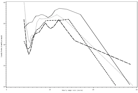
This speci…cation has the main advantage of allowing very ‡exible responses of hours to wage rate. To justify this ‡exibility, Figure 1 reports four locally weighted
regressions of female hours on the wage rate. The thick regression line relates to a sample of households with nonwife income below the …rst quartile. The dotted regression line relates to a sample of households with nonwife income above the …rst quartile and below the median. The dashed regression line relates to a sample of households with nonwife income above the median and below the third quartile and the large dashed regression line to a sample of households with nonwife income above the third quartile. A clear non-monotonic relationship between hours and wages appears. Moreover, for a given wage rate, the slope of this relationship depends on nonwife income. The di¤erent curves also show a substantial income e¤ect. Hence a ‡exible speci…cation is necessary to grasp these features.11
The collective model yields a set of parametric restrictions on (15) that can be empirically tested. Using the results given in Proposition 3, we can show that the coe¢ cients of this functional form have to satisfy the following restrictions:12
2a33a12 a13a23= a23a23 4a33a22= 0: (16)
Note that these restrictions do not entail unrealistic constraints on behavior. More-over, the Slutsky condition implies that
a01 a03a13 2a33 + 2 a11 a213 4a33 wf a02 a03a23 2a33 hf > 0: (17)
In principle, this restriction can be globally imposed but it reduces excessively the ‡exibility of the functional form. Hence we prefer checking (17) for each observation. Now, if these restrictions are imposed, the wife’s Marshallian labor supply and the sharing rule can be retrieved. And, from the results given in Proposition 4, the superiority of goods x and c can be tested.
11These results are only illustrative since no allowance is made for the endogeneity of the wage
or nonwife income. Note that the data are sparse for wf greater than 20.
Hour l y wage r at e ( eur os ) 20 25 30 35 40 0 10 20 30
Figure 1: Locally weighted regression, FHBS 2000 data
3.2
Recovering the Structural Parameters
Sharing rule. Let us de…ne = a03+ a23 + a13wf + 2a33x and = a03a23
2a02a33. The s-conditional sharing rule is quadratic and its derivatives are given by
@ @wf = a13 ; @ @ = a23 and @ @x = 2a33 .
Solving this system of three partial di¤erential equations, we obtain the s-conditional sharing rule equation:
= K0(z) + K1wf + K2 + K3x + K4wf2+ K5 2+ K6x2 (18)
+K7wf + K8wfx + K9 x;
where K0(z)is an unidenti…ed function of z, and where
K1 = a03a13 ; K2 = a03a23 ; K3 = 2a03a33 ; K4 = a2 13 2 ; K5 = a2 23 2 ; K6 = 2a2 33; K 7 = 2a12a33 ; K8 = 2a13a33 ; K9 = 2a23a33 :
It is also possible to recover the Marshallian labor supply associated with this setting.
Marshallian labor supply. The Marshallian labor supply does not depend on the conditioning good x and takes the following form:
where A(z) = a00(z) + a02 a03a23 2a33 K0(z); B = a01 a03a13 2a33 ; C = a11 a213 4a33 ; D = a02 a03a23 2a33 :
Hence the wife’s Marshallian labor supply belongs to the family of semi-quadratic speci…cations, and the normality of leisure implies that D < 0. Note that the utility function that rationalizes this functional form exists in closed form and is given by Stern (1986).
Slopes of the Engel curves. If goods x and c are superior, the slope of the Engel curves generates a strong test of collective rationality, as is explained in the discussion of Proposition 4. To carry out this test, these slopes have to be computed for the present functional form with the identi…cation results given in Proposition 2. However, the formulae are quite complicated, so that the slopes are not exhibited here. Note that the positivity must be checked for each observation since the Engel curves are not linear.
4
Data and Empirical Results
4.1
Data
The data are taken from the French Household Budget Survey 2000 conducted by the French institute of economic and statistical information (INSEE). It contains detailed information on consumption, labor income, working hours, education and demographic characteristics. We select a sample of married and cohabiting couples where the adults are aged between 20 and 60 and available for the labor market. For this purpose, households where adults are disabled, retired or students are excluded. We also exclude households where adults are self-employed or farmers. The labor supply behavior of these two categories may indeed be rather di¤erent from salaried workers and, altogether, would require a di¤erent modeling strategy. We further select households where hours of work are positive for wives and at least 35 hours per week for husbands. We also restrict our sample to households with no pre-school (under 3) children in order to minimize the extent of nonseparable public goods within the household which is not accounted for in our model. Finally, since Browning and Chiappori (1998) argue that the hypothesis of e¢ ciency in the intra-household decision process is more likely to be satis…ed in stable couples, we further
restrict our sample to households with at least two years of conjugal life. In all, these selection criteria lead us to 1670 observations.
Table 1: Descriptive Statistics of the Sample
Mean Median Std. Dev.
The Whole Sample of Working Couples
Male weekly hours of work 40:65 39:00 8:09
Female weekly hours of work 33:24 35:00 9:56
Our Selected Sample of 1670 Couples
Female weekly hours of work 33:33 35:00 9:64
Female hourly wage rate 8:78 7:71 4:18
Annual food expenditures 6101 5762 2810
Annual nonwife income 20632 16815 19479
Wife’s age 41:00 41:00 8:15
Number of children 1:28 1:00 1:08
Notes: all monetary amounts in euros.
The theory developed above requires the conditioning good x to be private and nondurable. In addition, since expenditures on nondurables are recorded in the sur-vey on diaries covering two-week periods (and extrapolated for the year), infrequency of purchases may be a serious issue. We thus choose the household expenditure on food at home (including alcohol and tobacco) as the conditioning good. One advan-tage of using that variable is that the number of zeros is far lower than for other goods. However, we have also estimated the model with two other conditioning goods, namely, food away from home and clothing. In this case, the collective re-strictions (16) and (17) are not rejected by the data but the coe¢ cients are less precisely estimated than with food at home as the conditioning good. These esti-mations are summarized in Table 6 (Appendix B).
The female labor supply hf is the number of working hours per week. The wage
rate wf is the average hourly earnings de…ned by dividing the wife’s total labor
income on all jobs over annual hours of work on all jobs. As the latter information is not included in the data, it is computed from hf and the number of months worked
during the year.
The nonlabor income y is de…ned as the nonlabor income net of savings and is given by the budget identity: y = c + x wmh wfhf, so that the nonwife
income is equal to: = c + x wfhf. That is, the nonwife income is the
di¤erence between annual household total consumption and female labor earnings. In doing that we follow Blundell and Walker (1986) and adjust nonwife income to be consistent with an intertemporally separable life-cycle model.
wife’s age.13 As in Bourguignon and Magnac (1990), the wife’s education level is
used as an excluded instrument, instead of being used as a regressor.
Some descriptive statistics of the sample are exhibited in Table 1. The …rst and second rows of the table help us compare the distribution of male and female labor supply for working couples. On average, men work more than women and their labor supply is more concentrated. The comparison with the United-States, for instance, is striking. In the PSID of 1990, using a similar selection as done here for couples, we …nd that there is no obvious concentration in the distribution of hours, apart from the mode between 35 and 40 weekly hours. This spike itself concerns only 39:5% (resp. 36:8%) of US men (resp. women) in working couples compared to 65:5% (resp. 45:9%) of the French men (resp. women) in working couples. We are inclined to believe that the variability in husbands’ working hours can simply be disregarded by a study of French wives’behavior. This issue is examined below with a formal test of the rigidity of male labor supply.
4.2
Endogeneity and Choice of Instruments
The wage rate is computed as labor income divided by hours of work. This may induce the so-called ‘division bias’. Moreover, the nonwife income and the food expenditures are likely to be endogenous as they are choice variables in the model. Therefore, we have chosen to instrument the wife’s wage rate, the nonwife income, the food expenditures and their squares and cross-products. The possible endo-geneity of children deserves further attention. On the one hand, we may assume that we only need to worry about the endogeneity of recently born children and can treat older children as predetermined. On the other hand, there is some evidence that labor force behavior surrounding the …rst birth is a signi…cant determinant of lifetime work experience (Browning, 1992). All things considered, this issue is an empirical one. Hence, since the exogeneity of the number of children is not rejected by our data, the estimations of the model we present below do not instrument the number of children.14
Now, an issue that requires some discussion relates to the choice of the instru-ments. We …rst assume that the husband’s annual labor earnings are not correlated with the wife’s taste for work. This is a reasonable assumption as, in our model, his labor supply is exogenously constrained. To grasp as much variation as possible
13In principle, the socio-demographic factors z may also include variables related to the husband.
However, these turn out to be insigni…cant.
14However, our conclusions are still valid when the number of children is supposed to be
endoge-nous. In that case the estimates di¤er only in that the coe¢ cient of the number of children in (15) is no longer signi…cant. These results are available upon request.
in the endogenous regressors, we use a fourth order polynomial in the husband’s labor earnings. We also use a second order polynomial in age and education for the wife and for the husband, and a second order polynomial in exceptional incomes (including inheritance, bequests and gifts) as instruments. This yealds sixteen in-struments.15
Other instruments include a constant, the number of children, two dummies for husband’s father’s profession, a dummy variable for living in the Paris region, a cross-term of wife’s education and husband’s labor earnings. Since our estimation technique takes account of the selection of the sample, we also use the inverse Mill’s ratio as an instrument. In all, we have twenty-three instruments. As usual, mea-surement error in the instruments is not supposed to be correlated with the response error for the endogenous variables.16
4.3
Results
Before we present any further results we report the tests of the validity of the instruments.
4.3.1 The validity of the instruments
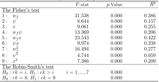
We …rst test the null hypothesis that none of the excluded instruments is correlated with the endogenous variables in the system of equations Y = W + e; where Y is the matrix of endogenous regressors, W the matrix of instruments and a matrix of parameters and e a matrix of random terms. The …rst panel of Table 7 in Appendix C shows F statistic, corresponding p-value and adjusted R-square for each of the nine auxiliary regressions. The p-values are close to zero, indicating that the null hypothesis is clearly rejected. This gives evidence that the instruments are signi…cant for all the endogenous variables. Note, however, that the F statistic concerning the auxiliary regression on 2 is relatively small (less than 5). In a 2SLS context Staiger and Stock (1997) suggest that estimates and con…dence interval may be unreliable with …rst-stage F ’s this small.17 On the other hand, Bound, Jaeger and
Baker (1995) mention that results should be interpreted with caution for …rst-stage F statistics close to one.
15These instruments are strongly correlated. To avoid this problem, we replace the
polynomi-als with their corresponding principal components, that is orthogonal linear combinations of the original instruments. Estimations are then more stable.
16For Altonji (1986) and Altonji and Siow (1987) this assumption is reasonable, given that these
variables are based on independent questions.
17We allow for heteroscedasticity of unknown form and estimate the model with GMM. We do
To decide on the potential weakness of our instruments, we test whether the excluded instruments have enough explanatory power jointly for all the endogenous variables. For that purpose we use the test provided in Robin and Smith (2000). This test evaluates the rank of the coe¢ cient matrix on the excluded instruments in the auxiliary regressions. A short account is in Blundell, Duncan and Meghir (1998). Let ^ be a consistent and asymptotically normal estimator of a p k reduced form parameter matrix on the excluded instruments.18 Here we have four
included instruments (a constant, the wife’s age, the number of children and the inverse of Mill’s ratio) so that there are p = 23 4 = 19 excluded instruments and k = 9 endogenous variables. If is not full rank (i.e., rk( ) < 9); the excluded instruments are weak for at least one endogenous variable. If is full rank (i.e., rk( ) = 9), the excluded instruments have enough explanatory power jointly for all the endogenous variables. The Robin-Smith test of rank is based on the eigen values of ^T^ .
Following the sequential procedure advocated in Robin and Smith (2000), we test for H0 : rk( ) = r against H1 : rk( ) > r for r = 1; :::; 9 and halt at the …rst
value of r for which the test statistic indicates a nonrejection of H0. The second
panel of Table 7 in Appendix C exposes the results. Again, the p-values are close to zero: The null hypothesis rk( ) = 1 is rejected, so is the null rk( ) = 2; and so on until rk( ) = 8 is also rejected: the reduced form coe¢ cient matrix is full rank. We thus conclude that the excluded instruments are valid enough to give reliable estimates and con…dence interval.
4.3.2 Tests of husband’s labor supply rigidity
Our theoretical results crucially rely on the postulate that the wife’s labor supply is independent of the husband’s wage rate (conditionally on the levels of nonwife income and one reference good). This is a consequence of the husband’s labor supply rigidity. In particular, if the husband’s hours of work vary, the wife’s labor supply will in general depend on the husband’s wage rate. In that case our conclusions will be invalidated.
As a matter of fact, the data indicates that the dispersion of the husband’s working hours is quite limited. In spite of that the husband’s wage rate can possibly in‡uence the wife’s behavior and question the validity of our approach. Also, the rigidity of the husband’s behavior must be tested. To do that, we introduce an additional term, wm, in (15) and assess its signi…cance.19 We perform this test 18The matrix contains only the parameters of related to the excluded instruments in the
s-conditional labor supply equation.
whether Wm is included or not in the set of instruments, where Wm is the matrix of
variables constructed from the husband’s labor income. In both cases the husband’s wage rate has no impact statistically di¤erent from 0.
We also test in the estimation of (15) for the endogeneity of the subset of in-struments Wm. Suppose that the husband’s wage rate is exogenous. Now it is
orthogonal to the error term if husband’s labor supply is exogenously constrained. Otherwise it is not. The corresponding test statistic is simply the di¤erence in the criterion functions for GMM estimation with and without the questionable instru-ments Wm (Ruud, 2000, p. 576). Under the null hypothesis of orthogonality it
converges in distribution to a 2(k) random variable, where k = 5 is the number of questionable instruments. The di¤erence gives a test statistic of 8:139 (8:115 if the collective restrictions (16) are imposed). At conventional levels we do not reject the null hypothesis.20 In conclusion, even if the husband’s working hours exhibit some
dispersion, this should not prevent us from applying the present theory. In addi-tion this test reinforces the evidence that the husband’s labor supply is exogenously determined in France.
4.3.3 Labor supply estimates
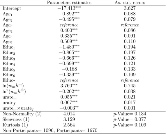
Firstly, conditioning the sample on “stable” households with working wives and no children under 3 year of age may induce a selectivity bias. To account for all these selection rules we estimate a reduced-form participation equation and include the inverse Mill’s ratio into the labor supply equation (15). The estimates of the selection equation are shown in Table 8 (Appendix C). This equation includes the wife’s age and education, the husband’s income and male and female unemployment rates as explanatory variables. The results show a strong e¤ect of age, education and income, whereas the unemployment rates have a signi…cant e¤ect. Hence the labor supply equation, which excludes the latter variables, is well identi…ed.
Let us now turn to the labor supply results. We denote the inverse Mill’s ratio estimated from the participation equations by ^ and the matrix of residuals obtained from the regression of the variables on the instruments (i.e., Y = W + e) by be. The …rst and third columns of Table 2 provide estimates of the unrestricted and restricted models obtained by applying OLS (NLS) on the following relation:
hf = g(wf; ; x; z; a) + ^b + ^ebe+ v; (20)
where g( ) is the functional form (15) of the wife’s labor supply, v is a random term
explicitly intended to test the implication of the dispersion in husband’s working hours that may invalidate our theory.
Table 2: Estimated Parameters of the Reduced Form Labor Supply
Unrestricted Model Restricted Model
OLS GMM NLS GMM a01: wf 4:430 4:727 4:190 4:501 (1:082) (1:109) (0:976) (0:989) a02: 10 2 0:105 0:104 0:093 0:095 (0:059) (0:059) (0:042) (0:039) a03: x 0:003 0:003 0:004 0:004 (0:003) (0:003) (0:002) (0:002) a11: wf2 0:106 0:118 0:122 0:125 (0:056) (0:054) (0:044) (0:042) a22: 2 10 9 4:044 4:531 3:589 4:121 (3:031) (2:782) (2:446) (2:171) a33: x2 10 8 9:548 11:910 6:458 8:656 (19:687) (19:780) (5:430) (5:579) a12: wf 10 2 0:005 0:006 0:006 0:006 (0:005) (0:005) (0:003) (0:003) a13: wfx 10 2 0:032 0:033 0:026 0:029 (0:020) (0:019) (0:018) (0:017) a23: x 10 9 1:374 18:600 30:450 37:800 (89:958) (92:490) (20:521) (18:600) 0 : Intercept 21:231 18:255 17:932 16:137 (9:444) (9:545) (6:946) (7:051) ch : Number of children 1:415 1:393 1:556 1:462 (0:718) (0:705) (0:642) (0:623)
age : Wife’s age 0:257 0:275 0:261 0:274
(0:089) (0:085) (0:085) (0:079)
b : Inverse Mill’s ratio 1:880 2:472 2:428 2:848
(2:276) (2:306) (2:039) (2:059) bewf : bewf 3:433 3:193
(1:126) (1:021)
Objective function 9:393 9:548
Notes: Asymptotic standard errors in parentheses. Signi…cance levels of 10, 5 and 1% are noted *, ** and *** respectively.
which represents the unobserved heterogeneity, and a; b and be are parameters.
The inclusion of the residuals in the labor supply equation is to control for the endogeneity of the regressors. It also provides a direct test of exogeneity. These are the t statistics of the estimates of be; see Smith and Blundell (1986) or Blundell,
Duncan and Meghir (1998) for a recent application. The asymptotic covariance matrix is computed using the results of Newey (1984) and Newey and McFadden (1994) to take into account that we are conditioning on generated regressors (i.e., ^ and ^e).21 It is robust to heteroskedasticity of unknown form. To save space, only the
test of exogeneity for the wife’s wage rate is reported in Table 2. The wife’s wage rate is likely to be measured with error and unobserved individual characteristics may be correlated with it. The residual of the regression of the wife’s wage rate on the instruments is denoted by ^ewf. Then, under the null hypothesis, the parameter
bewf corresponding to the residual ^ewf in equation (20) must be equal to zero. This
is clearly rejected by the data. The wage rate has to be instrumented.
The second and fourth columns of Table 2 are the unconstrained and constrained models obtained by using GMM on the following equation:
hf = g(wf; ; x; z; a) + ^b + : (21)
The Hansen’s test does not reject the validity of the instruments and the overidenti-fying restrictions. The test statistics 9:393 and 9:548 are less than the critical values of the 2
0:05(10) = 18:307 and of the 20:05(12) = 21:026. Note that, except for the
interaction term x, the OLS and GMM estimations give similar results. How-ever, under the presence of heteroskedasticity of unknown form, the GMM estimator attains greater e¢ ciency (Davidson and MacKinnon, 1993, p. 599). Therefore, we only refer to the GMM results in what follows.
Let us take a closer look at the results of Table 2. We note that the parameters of the unrestricted model are not estimated with precision. Only the wife’s age, the number of children, the wage rate, its square, its interaction with food expenditures and the nonwife income have an impact at the 5% or 10% level. This lack of precision can be explained by the ‡exibility of our functional form. Nonetheless, the coe¢ cients of the restricted model (i.e., with the imposition of conditions (16)) are very similar, but exhibit smaller standard errors, so that most of them are statistically signi…cant at the 5% or 10% level. In particular the wife’s age and the number of children have a signi…cant, negative e¤ect on the number of working hours. Moreover, the inverse Mill’s ratio does not in‡uence wife’s labor supply. Apparently, the selection of the sample is not a serious issue.
21We account for the covariance of the coe¢ cients ^ across the nine reduced forms. Still, we
We now turn to the test of the collective restrictions. To begin with, we perform a Newey-West’s test of conditions (16). Since the di¤erence in the function values (i.e., 9:548 9:393 = 0:155) is much smaller than the critical value, 20:05(2) = 5:99,
we do not reject the restrictions at stake. However, this evidence in favor of the collective model must be interpreted with caution. Indeed, the standard error of the coe¢ cient a33 is large. Since this coe¢ cient enters conditions (16), the test we carry
out is not likely to be powerful. Also, the other tests at our disposal are essential to assess the validity of the model.
Using the estimates of the restricted model, we note that the Slutsky condition (17) is satis…ed for a large majority (93%) of the households in the sample, and the wife’s leisure is superior.22 These results support the collective model and they
will be more closely examined below. In addition, the positivity of the slopes of the Engel curves can be checked since it is reasonable to assume that both goods are superior. This corresponds to a test of the second statement in Proposition 4. Actually we observe that the slopes of the four Engel curves are positive for 95:45% of the households in the sample. This con…rms that the goods are superior and, incidentally, valid our estimations.
On the whole, the empirical tests we describe above do not reject the collective model concerned. Let us now consider various labor supply elasticities. These are shown in Table 3. The elasticities of the constrained and unconstrained models are similar and quite precisely estimated. Women’s wage elasticities are positive and statistically signi…cant. Income elasticities are negative and also statistically signif-icant. The amplitude of these …gures is somewhat di¤erent from that found with French data. For example, estimating a unitary model that accounts for non-linear taxation and nonparticipation, Blundell and Laisney (1988) report, at the sample mean, wage and income elasticities which are equal to 2 and 0:7 respectively. Ac-cording to the speci…cation used, these elasticities range from 0:05 to 1 respectively and from 0:3 to 0:2 in Bourguignon and Magnac (1990). The elasticities pre-sented in Table 3 di¤er from previous estimations because our sample is restricted to working wives.
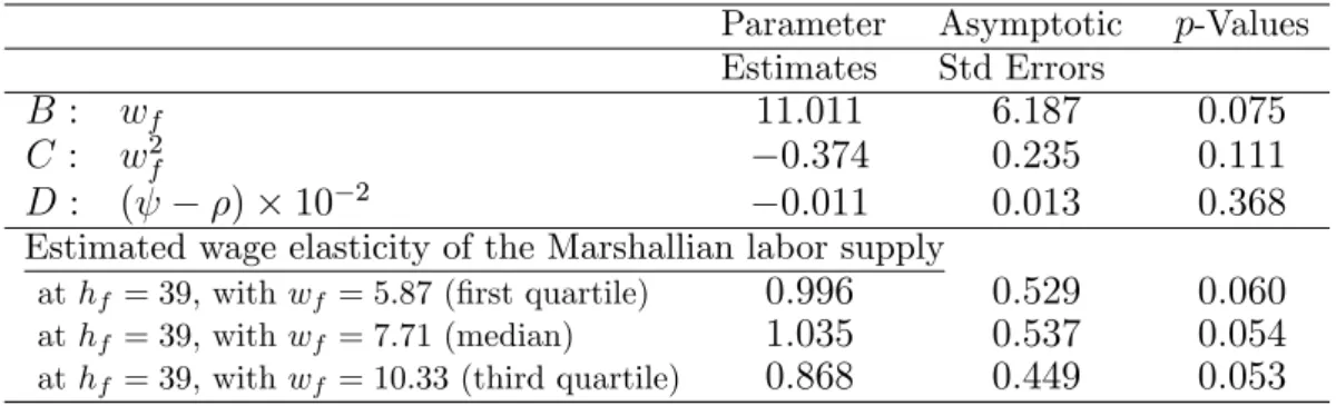
The estimation of the reduced form parameters allows us to retrieve some struc-tural components of the model. The …rst panel of Table 4 reports the estimates of the parameters of the Marshallian labor supply (19). The coe¢ cients have the expected signs but the e¤ect of the wife’s share of income is imprecisely estimated. Note also that the wife’s Marshallian labor supply is backward bending. For small values of the wife’s wage rate the substitution e¤ect dominates the income e¤ect so
22Remember that the Marshallian labor supply is linear in income. Hence the superiority of
Table 3: Elasticities of labor supply
Estimates Asymptotic Std. Errors p-Values
Estimated wage elasticity of the unconstrained labor supply
at wf = 5:87 (…rst quartile) 0:374 0:103 0:000
at wf = 7:71 (median) 0:405 0:102 0:000
at wf = 10:33 (third quartile) 0:379 0:089 0:017
Estimated wage elasticity of the constrained labor supply
at wf = 5:87 (…rst quartile) 0:386 0:086 0:000
at wf = 7:71 (median) 0:416 0:088 0:000
at wf = 10:33 (third quartile) 0:384 0:083 0:000
Estimated income elasticity of the unconstrained labor supply
at = 9842 (…rst quartile) 0:143 0:057 0:012
at = 16815 (median) 0:217 0:084 0:009
at = 27341 (third quartile) 0:286 0:106 0:007
Estimated income elasticity of the constrained labor supply
at = 9842 (…rst quartile) 0:136 0:049 0:006
at = 16815 (median) 0:207 0:074 0:005
at = 27341 (third quartile) 0:276 0:098 0:005
Notes: Asymptotic standard errors are computed with the Delta method. Elasticities are computed at hf = 39: Other covariates are at the sample mean.
Table 4: Estimated Parameters of the Structural Model: The Marshallian Labor Supply
Parameter Asymptotic p-Values
Estimates Std Errors
B : wf 11:011 6:187 0:075
C : w2
f 0:374 0:235 0:111
D : ( ) 10 2 0:011 0:013 0:368
Estimated wage elasticity of the Marshallian labor supply
at hf= 39; with wf = 5:87 (…rst quartile) 0:996 0:529 0:060
at hf= 39; with wf = 7:71 (median) 1:035 0:537 0:054
at hf= 39; with wf = 10:33 (third quartile) 0:868 0:449 0:053
Table 5: Estimated Parameters of the Structural Model: The Sharing Rule
Parameter Estimates Std. Error p-Value
K1 : wf 56923:450 84039:060 0:498 K2 : 7:317 10:105 0:469 K3 : x 33:532 41:789 0:422 K4 : w2f 2180:998 2933:883 0:457 K5 : 2 10 3 0:036 0:047 0:440 K6 : x2 10 3 0:757 0:811 0:351 K7 : wf 0:561 0:660 0:396 K8 : wfx 2:569 2:764 0:353 K9 : x 10 2 0:033 0:038 0:382
Estimated marginal impact of wf on the sharing rulea
at wf = 5:87 (…rst quartile) 35436:950 53190:582 0:505
at wf = 7:71 (median) 27415:070 42778:054 0:522
at wf = 10:33 (third quartile) 15984:050 28432:382 0:574
Estimated marginal impact of on the sharing rulea
at = 9842 (…rst quartile) 3:699 5:690 0:516
at = 16815 (median) 3:197 5:061 0:528
at = 27341 (third quartile) 2:438 4:123 0:554
Estimated marginal impact of x on the sharing rulea
at x = 4136 (…rst quartile) 10:415 16:930 0:538
at x = 5762 (…rst quartile) 12:876 19:291 0:504
at x = 7694 (…rst quartile) 15:800 22:177 0:476
Notes: Asymptotic standard errors are computed with the Delta method. a :Other covariates are at the sample mean.
that an increase in the wife’s wage rate has a positive impact on the working hours. For large values of the wife’s wage rate the converse is true. Then the rejection of Slutsky positivity appears for some households in which the wife is characterized by a very large wage rate. The second panel of Table 4 includes the wage elasticity conditional on the sharing of nonwife income. This ignores any e¤ect the wage rate may have on the intra-household decision process. We note that the wage elasticity is positive, concave and statistically signi…cant at the 10% level. It is twice as big as those reported in Table 3 and is close to one at the mean of the sample. It is noteworthy that this …gure may be compared with what is found in the literature on collective models. For example, Chiappori, Fortin and Lacroix (2002) report a wage elasticity of 0:178 with United States data, Fortin and Lacroix (1997) a wage elasticity of 0:361 with Canadian data, and Moreau and Donni (2002) a wage elas-ticity of 0:394 with French data. The elasticities in Table 4 are substantially greater. However, they are compatible with previous researches since the standard errors of the estimated parameters are quite large. Finally, the sharing rule estimates are shown in the …rst panel of Table 5. The parameters turn out not to be precisely estimated. No coe¢ cient is signi…cant at the 10% level. In the second panel of Table 5, the marginal impacts of the exogenous variables on the sharing rule are presented but the estimates are still imprecise.
5
Conclusion
In the present paper we suppose that the husband’s labor supply is exogenously determined. We then advocate a simple approach to model the wife’s labor supply, in which the wife’s behavior is explained by her wage rate, other household incomes, socio-demographic variables and the demand for one good consumed at the house-hold level. In this approach the level of the conditioning good can be interpreted as an indicator of the distribution of power within the household.
We then demonstrate that the estimation of a single equation (including one conditioning good as argument) permits to carry out tests of collective rationality and to identify some elements of the structural model. The simplicity of the esti-mation method suggests that the approach used in this paper is specially pro…table to perform empirical tests.
Another important contribution of the present paper is to show that our approach (and the collective setting as a whole for that matter) is compatible with domestic production on the condition that the household production function belongs to some speci…c family of separable technologies.
using a French sample of working wives. We show that, overall, the collective re-strictions are satis…ed by the data. However, the estimates of the structural model are not precisely estimated. One way of dealing with that is to exploit the infor-mation on nonparticipating wives. Indeed, the parameters that enter the ‘reduced’ participation equation (used in constructing the inverse Mill’s ratio) are not related to the parameters of the labor supply equation. In that case, the basic idea is to estimate a ‘structural’participation equation, derived from the comparison of a shadow wage equation (incorporating the parameters of the wife’s labor supply) and a market wage equation. The implementation of this idea raises some econometric di¢ culties, though. This is the topic of future work.
Appendix A : Proof of Propositions
Proof of Proposition 2
1. Identi…cation of @ m=@ . Di¤erentiating the s-conditional labor supply with respect to and x gives:
@hf @ = @ f @ ( ) 1 @ @ ; @hf @x = @ f @ ( ) @ @x: Since @hf=@ 6= 0 from R, this yields:
@hf @ @hf @x 1 = 1 @ @ @ @x 1 : (22)
Similarly, using Lemma 1 and di¤erentiating the household demand for good x with respect to and x gives:
1 = @ m @ @ f @ ( ) @ @x; (23) @ m @ = @ m @ @ f @ ( ) 1 @ @ (24) or @ m @ = 1 @ @ @ @x 1 (25) Substituting (22) in (25) yields the husband’s Engel curve:
@ m @ = @hf @ @hf @x 1 = : (26)
2. Identi…cation of @ =@wf, @ =@ and @ =@x. Di¤erentiating (26) with
re-spect to wf, and x yields:
@2 m @ 2 @ @wf = @ @wf , @ 2 m @ 2 @ @ = @ @ , @2 m @ 2 @ @x = @ @x. Since @ @ @hf @x 6= @ @x @hf @ ;
this system of partial di¤erential equations, together with (22), can be solved with respect to @ =@wf, @ =@ and @ =@x. That is,
@ @wf = @ @wf , @ @ = @ @ , @ @x = @ @x . (27)
3. Identi…cation of @ f=@( ) and @ f/@wf. If we di¤erentiate the wife’s
s-conditional labor supply with respect to x and wf, we obtain:
@hf @x = @ f @( ) @ @x; @hf @wf = @ f @wf @ f @( ) @ @wf : (28)
Since 6= 0 and @ =@x 6= 0, substituting (27) in (28) yields: @ f @( ) = @hf @x 1 (@ =@x); @ f @wf = @hf @wf @hf @x @ =@wf @ =@x : (29)
4. Identi…cation of @ f=@( ) and @ f=@wf. The slopes of the demand for
good x can be retrieved in a similar way. Substituting (26) and (27) in (23) gives: @ f
@ ( ) =
1
(@ =@x): (30) Di¤erentiating the household demand for good x with respect to wf, and using (26)
and (27) yield:
@ f @wf
= @ =@wf @ =@x :
5. Identi…cation of other elements. The derivatives of the Marshallian de-mands for good c can be obtained from the individual budget constraints. Moreover, once the function k(z) is picked up, the wife’s total consumption can be retrieved. Then, the wife’s utility function is derived as usual.
Proof of Proposition 3
1. Substituting (29) in (8) yields: @hf @wf @hf @x @ =@wf @ =@x hf (@ =@x) > 0:2. From the Young’s Theorem, the derivatives of the sharing rule have to satisfy a symmetry restriction. Simplifying yields:
@ @wf @ @x @ @x @ @wf = @ @ @ @x @ @x @ @ = 0:
Proof of Proposition 4
1. From (29), @hf=@x (@ =@x) > 0;if wife’s leisure is normal. This gives the …rst statement in Proposition 4.
2. From (26) and (30),
> 0, 1
(@ =@x) > 0;
if good x is normal (for both spouses). From these expressions and the individual budget constraints, we obtain:
1 @ m @ = 1 > 0; 1 @ f @( ) wf @ f @( ) = 1 + 1 + wf(@hf=@x) (@ =@x) > 0:
if good c is normal (for both spouses). Rearranging these expressions gives the second statement.
Appendix B : Alternative Estimations
We carry out two alternative estimations of the model, with expenditures on food away from home and clothing as the conditioning good respectively. One problem, however, is that reported expenditures on clothing (resp. food away from home) are equal to zero for 7:5% (resp. 18%) of the 1670 households of our selection. Be that as it may, these estimations are presented in Table 6. For the sake of comparability, the estimated parameters are obtained with the same set of instruments as those used for the regression in the main text. To complete these results, note that the parameters B and C of the Marshallian labor supply are signi…cant at the 1% level when the conditioning good is food away from home; in that case, the parameters K6 and K9 are also signi…cant (at the 5% and the 10% level). Furthermore, the
Slutsky condition is satis…ed for 92% of the sample, while conditions (a) and (b) of Proposition 4 are satis…ed for 100% and 34% of the sample respectively. On the other hand, when the conditioning good is clothing, the results are less convincing. No parameters of the structural model are signi…cant. The Slutsky condition is satis…ed for 66% of the sample, and the conditions (a) and (b) are satis…ed for 100 %and 8% of the sample respectively.
Table 6: Estimation with two alternative conditioning goods
Unrestricted Model Restricted Model
Food away Clothing Food away Clothing
from home from home
a01 wf 5:406 5:104 4:169 4:018 (2:801) (1:881) (1:738) (1:021) a02 10 2 0:059 0:054 0:068 0:043 (0:050) (0:044) (0:041) (0:032) a03 x 0:001 0:003 0:002 0:000 (0:007) (0:006) (0:004) (0:004) a11 wf2 0:207 0:222 0:142 0:139 (0:106) (0:092) (0:050) (0:040) a22 2 10 9 5:879 2:504 6:010 2:394 (2:969) (2:896) (2:751) (2:130) a33 x2 10 8 60:380 25:920 48:680 1:984 (52:380) (50:360) (41:230) (9:804) a12 wf 10 2 0:002 0:005 0:002 0:002 (0:003) (0:004) (0:003) (0:003) a13 wfx= 10 2 0:017 0:031 0:017 0:006 (0:050) (0:041) (0:022) (0:021) a23 x 10 9 193:000 134:000 108:00 13:800 (132:400) (111:600) (59:570) (34:550) 0 Intercept 15:673 19:564 22:412 23:100 (14:619) (10:231) (10:146) (6:109)
chi Number of children 0:244 1:019 0:162 1:169
(0:868) (0:979) (0:766) (0:768)
age Wife’s age 0:150 0:144 0:159 0:151
(0:062) (0:059) (0:051) (0:046)
b Inverse Mill’s ratio 3:355 1:599 1:924 0:974
(3:624) (2:239) (2:815) (1:811)
Objective function 6:391 7:4373 8:383 12:263
Notes: Asymptotic standard errors in parentheses. Signi…cance levels of 10, 5 and 1% are noted *, ** and *** respectively.
Appendix C : Auxiliary Regressions and Selection
Equation
Table 7: Tests of the Validity of the Instruments
F-stat p-Value R2
The Fisher’s test
1 : wf 31:538 0:000 0:386 2 : 8:644 0:000 0:157 3 : x 9:061 0:000 0:255 4 : wf 13:369 0:000 0:206 5 : wfx 23:543 0:000 0:422 6 : x 9:974 0:000 0:238 7 : w2 f 16:494 0:000 0:277 8 : 2 4:744 0:000 0:059 9 : x2 7:386 0:000 0:209
The Robin-Smith’s test
H0 : rk = i; H1 : rk > i i = 1; :::; 7 0:000
H0 : rk = 8; H1 : rk = 9 0:000
In Table 8, the wife’s age is represented by dummies, Agei with i = 1; :::; 6. The
age groups are < 30, 31 34, 35 39, 40 44, 45 49and 50. The wife’s education level is also represented by dummies, Educi, with i = 1; :::; 7, which represent the
highest diploma attained by the wife. The unemployment rate is speci…c to gender and varies with age and education. It is denoted by uratei, with i = m; f . The
statistics for the normality test is equal to 4:014 (with two degrees of freedom) which is acceptable at conventional levels.
Table 8: Reduced Form Participation Probit
Parameters estimates As. std. errors
Intercept 17:413 3:627
Age1 0:892 0:088
Age2 0:495 0:079
Age3 reference reference
Age4 0:400 0:086 Age5 0:335 0:091 Age6 0:509 0:110 Educ1 1:480 0:194 Educ2 0:865 0:197 Educ3 0:666 0:126 Educ4 0:699 0:121 Educ5 0:188 0:133 Educ6 0:339 0:109
Educ7 reference reference
ln(wmhm) 3:760 0:745 ln2(wmhm) 0:202 0:038 uratem 0:055 0:021 uratef 0:067 0:017 uratem uratef 0:003 0:001 Non-Normality (2) 4:014 p-Value= 0:134 Skewness(1) 3:129 p-Value= 0:077 Kurtosis (1) 2:564 p-Value= 0:109 Non-Participants= 1096,Participants= 1670
Note: Signi…cance levels of 10, 5 and 1% are noted *, ** and *** respectively. The statistics of tests have a 2 distribution (degrees of freedom are in parentheses). The normality test statistics reported here follow the Generalised Residual methodology of Chesher and Irish (1987).
References
Altonji J. G. (1986), “Intertemporal Substitution in Labor Supply: Evidence from Micro Data”, Journal of Political Economy 94 : S176–S215.
Altonji J. G. and A. Siow (1987), “Testing the Response of Consumption to Income Changes with (Noisy) Panel Data”, The Quarterly Journal of Economics 102 : 293– 328.
Apps P.F. and R. Rees (1997), “Collective Labour Supply and Household Produc-tion”, Journal of Political Economy 105 : 178–190.
Bloemen H.G. (2004), “An Empirical Model of Collective Household Labor Supply with Nonparticipation”, Working Paper 010/3, Tinbergen Institute.
Blundell R. and F. Laisney (1988), “A Labour Supply Model for Married Women in France: Taxation, Hours Constraints and Job Seekers”, Annales d’économie et de statistique 11: 41-71.
Blundell R. and I. Walker (1986), “A Life Cycle Consistent Empirical Model of Labour Supply Using Cross Section Data”, Review of Economic Studies 53 : 539– 558.
Blundell R., A. Duncan and C. Meghir (1998), “Estimating Labor Supply Responses Using Tax Reforms”, Econometrica 66 : 827-861.
Blundell R., P.-A. Chiappori, T. Magnac and C. Meghir (2004), “Collective Labour Supply : Heterogeneity and Nonparticipation”, Mimeo, University College of Lon-don.
Bound J., D. A Jaeger and R. M. Baker (1995), “Problems with Instrumental Vari-ables Estimation When the Correlation Between the Instruments and the Endoge-nous Explanatory variable is Weak”, Journal of the American Statistical Association 90: 443-450.
Bourguignon F. and T. Magnac (1990), “Labor Supply and Taxation in France”, The Journal of Human Resources 25: 358-389.
Bourguignon F., M. Browning, P.A. Chiappori (1995), “The Collective Approach to Household Behaviour”. Working Paper DELTA 95/04.
Browning M. (1992), “Children and Household Economic Behavior”, The Journal of Economic Literature 30: 1434-1475.
Browning M. (1998), “Modelling Commodity Demands and Labour Supply with m-Demands”. Working Paper University of Copenhagen.
Browning M. and C. Meghir (1991), “The E¤ects of Male and Female Labor Supply on Commodity Demand”, Econometrica 59 : 925–951.