An analytical framework for rapid estimate of rain rate during tropical cyclones

1

An Analytical Framework for Rapid Estimate of Rain Rate

1

during Tropical Cyclones

2

Reda Snaiki, Teng Wu

*

3

Department of Civil, Structural and Environmental Engineering, University at Buffalo, State

4

University of New York, Buffalo, NY 14126, USA

5

*_{Corresponding author. Email: [email protected]}

6

Abstract: An analytical framework for rapid estimate of rain rate during a translating tropical

7

cyclone was proposed in this study. The efficient analysis framework for rain field is based on the

8

observation that rain-induced momentum flux at Earth’s surface cannot be ignored. The total

9

surface stress results mainly from momentum flux contributions of wind and rain. A

height-10

resolving wind field was utilized during the model construction leading to a linear, analytical

11

solution of the surface rain rate. The obtained rain rate model explicitly depends on parameters for

12

a typical tropical cyclone wind field simulation, namely storm location, approach angle, translation

13

speed, radius of maximum wind, pressure profile, surface drag coefficient, and turbulent

14

diffusivity. Hence, it could be readily implemented into state-of-the-art tropical cyclone risk

15

assessment using the Monte Carlo technique. The rainbands in the proposed methodology were

16

simulated using a local perturbation scheme. Sensitivity analysis of the rainfall field to the

17

abovementioned parameters was comprehensively conducted. The results generated by the present

18

analytical framework for rapid estimate of rain rate during tropical cyclones are consistent with

19

field measurements.

20

Keywords: Tropical cyclone, rain rate, wind field simulation, rain-induced stress.

21 22

2

1. Introduction

23

Tropical cyclones are responsible for the substantial part of natural hazard-induced economic and

24

life losses through high winds, torrential rain and wind-driven storm surge. Among these, the

25

rainfall-induced inland flooding contributes to a significant portion of the tropical cyclone related

26

damages (e.g., Landsea 2000; Rappaport 2000). Therefore, the rain field simulation inside the

27

tropical cyclone has attracted interest of a number of researchers for a better rainfall hazard

28

assessment. While there have been considerable advances in improving the simulation accuracy

29

of tropical cyclone rain field based on high-fidelity numerical weather prediction models, they are

30

not practical for risk assessment due to their high computational demands. Usually, the rainfall

31

distribution can be efficiently characterized based on probabilistic, parametric or physically-based

32

schemes.

33

The probabilistic models give good insights on the exceedance rate of specific rainfall

34

intensities, and are often used to predict the extreme rain rates. The development of this type of

35

models usually suffer from a lack of a large number of historical data that are needed to fit the

36

selected distributions. In addition, they are generally unable to represent the most important

37

physics governing the rain field inside the tropical cyclone (e.g., sea surface temperature, moisture

38

distribution, vertical wind shear, hurricane intensity and translational velocity). Actually, no

39

physical justification has been provided for the use of the popular distributions such as lognormal,

40

mixed-exponential and Gamma curves to fit the data (e.g., Woolhiser and Roldan 1982; Groisman

41

et al. 1999; Wilson and Toumi 2005).

42

The construction of the parametric models also requires a huge amount of rain field

43

measurements. Recently, the Tropical Rainfall Measuring Mission (TRMM) (Huffman et al.,

3

2010), a joint satellite mission of the National Aeronautics and Space Administration (NASA) and

45

the Japan Aerospace Exploration Agency (JAXA), has released a significant amount of tropical

46

cyclone rainfall data. The goal of TRMM is to provide good estimates of global precipitation using

47

satellite observations. TRMM contains several instruments, namely the TRMM Microwave

48

Imager (TMI), the Precipitation Radar (PR), the Visible Infrared Scanner (VIRS), the Lightning

49

Imaging Sensor (LIS), and the Clouds and Earth's Radiant Energy System (CERES). Details of the

50

TRMM instruments are given in Kummerow et al. (1998). Several empirical models have been

51

developed based on the TRMM database. For example, Lonfat et al. (2004) acquired the spatial

52

distribution of the rain field over the ocean using the TMI data from 1998 to 2000. The rain rates

53

were found to be heavily dependent on the sustained surface wind speed. The rain rate achieved

54

the maximum value near the radius of maximum winds and then decayed exponentially. According

55

to the hurricane intensities grouped into three categories, i.e., tropical storms, category 1-2 tropical

56

cyclones, and category 3-5 tropical cyclones, different radial variations of the rain rate were

57

obtained. Based on the findings from Lonfat et al. (2004) together with the surface rain gauge data,

58

Tuleya et al. (2007) proposed the Rainfall Climatology and Persistence (R-CLIPER) model. In this

59

parametric model, the rain rate presented a Rankine-like profile with a linear variation from the

60

tropical cyclone center to the radius of maximum rain rate, followed by an exponential decay. In

61

addition, it has been proved using the findings of Kaplan and DeMaria (1995) that the hurricane

62

rain rates and wind speeds are always highly correlated before/after landfall. While the R-CLIPER

63

model could be employed over both the ocean and land, it assumed a symmetric distribution of the

64

rain rate inside the tropical cyclone. Lonfat et al. (2007) improved the spatial variation of the rain

65

field by introducing a modified version of the R-CLIPER model known as the Parametric

66

Hurricane Rainfall Model (PHRaM) with consideration of the wind shear effects. However, both

4

the R-CLIPER and PHRaM models were found to underestimate the maximum rain rate since they

68

are based on the ensemble averages of numerous hurricanes (Tuleya et al. 2007).

69

Very few physics-based rain rate models have been introduced in the technical literature.

70

In the theoretical model proposed by Langousis and Veneziano (2009a), it is assumed that all the

71

upward moisture flux at the top of the tropical cyclone boundary layer is converted into rainfall.

72

The vertical moisture flux was evaluated from the vertical winds at a reference height, generated

73

by a modified version of the wind field model proposed by Smith (1968), along with the

depth-74

averaged temperature and saturation ratio. Although observations from Hurricane Frances

75

presented a maximum correlation (around 0.85) between the surface rain and vertical wind at an

76

elevation of 2-3 km, more comprehensive data may be necessary for the selected reference height.

77

Also, it is not easy to implement the modified version of Smith’s non-linear model in the Monte

78

Carlo technique with a large number of simulations needed. While the model by Langousis and

79

Veneziano (2009a) has been demonstrated to provide good estimates of the tropical cyclone rain

80

rate, it cannot account for post landfall scenarios.

81

In this study, a new, analytical framework for tropical cyclones rain rate estimate will be

82

developed for high-efficiency simulations. The rain rate analysis framework is based on the

83

observation that rain-induced momentum flux at Earth’s surface cannot be ignored (e.g., Caldwell

84

and Elliot 1971; 1972; Zhao et al. 2013). The total surface stress results mainly from momentum

85

flux contributions of wind and rain. A general formula of the rain intensity has been first derived

86

in which the iteration approach was utilized in the computation. The proposed methodology is able

87

to effectively integrate an efficient wind field model for rapid estimation of rain intensity during

88

tropical cyclones. Specifically, a height-resolving scheme recently developed by Snaiki and Wu

89

(2017a; 2017b) was utilized leading to a linear, analytical solution of the surface rain rate. The

5

rainbands in the proposed methodology were simulated using a local perturbation scheme (e.g.,

91

Samsury and Zipser 1995; Holland et al. 2010; Li and Wang 2012). Sensitivity analysis of the

92

rainfall field to several essential parameters in the rain rate simulation was comprehensively

93

conducted. The present analytical framework for rapid rain rate estimation has been validated

94

using observation data obtained from various hurricanes.

95

2. An analytical framework for rain rate estimation

96

The heat and moisture fluxes that are considered as the fuel and the surface stress contributing to

97

the dissipation essentially govern the intensity of a tropical cyclone (Chen et al. 2007), as

98

illustrated in Fig. 1.

99

100

Fig. 1. Major processes governing tropical cyclone intensity

101 102

In this study, the modeling of rain intensity is based on the dissipation process of tropical cyclones

103

where the total momentum flux is decomposed into several stress contributions. The general

104

practice to consider the total surface shear stress or equivalently the momentum flux density  is

105

based on the following parameterization (Andreas 2004; Donelan et al. 2004; Jarosz et al. 2007;

106 Huang 2012): 107 2 * au effective   (1) 108

6

where u_*effective= effective frictional velocity during rain; and a = air density. This

109

parameterization has been used in a number of applications such as the Fifth-generation

110

Pennsylvania State University–National Center for Atmospheric Research Mesoscale Model

111

(MM5) and the fully coupled atmosphere–wave–ocean model (AWO) (e.g., Chen et al. 2013).

112

Furthermore, the effective frictional velocity can be related to the effective drag coefficient

113

, d effective

C and the wind speed Vwindbased on the following formula:

114

2 2

* effective d effective wind,

u C V (2)

115

Therefore, the total shear stress can be expressed as:

116 2 , aCd effective windV   (3) 117

The square law as indicated in Eq. (3) has been comprehensively validated, especially at high wind

118

speeds, with a number of observations (Garratt 1977).

119

Various factors may contribute to the total surface stress, namely the turbulent fluxes, rain

120

effects, spray, airborne sediment (Saltation theory) and convection-induced stress. It is assumed

121

here that no airborne sediment exists, therefore its momentum flux contribution is disregarded as

122

well as the convection-induced stress (Huang 2012). The spray actually does not add extra

123

momentum to the system but redistributes the wind stress near the surface (Andreas 2004). Since

124

the droplets around the spray evaporate quickly (Emanuel 1995), its contribution is typically

125

negligible (e.g., Wu 1973; Fairall et al. 1994). On the other hand, the rain-induced momentum flux

126

can be significant as the raindrops interact with the near-surface wind and transfer momentum to

127

the surface (Caldwell and Elliot 1971; 1972). Zhao et al. (2013) compared the rain-induced

128

horizontal stress and the wind stress at various wind speeds and rain rates. It was demonstrated

7

that the horizontal stress by rain can have the same order of magnitude with that by wind.

130

Therefore, it is important to consider the rain-induced stress contribution to the total stress near

131

the surface. The total stress is then partitioned between two momentum contributions as:

132

a r

    (4)

133

where _a = momentum flux contribution from wind; and _r= momentum flux contribution from

134

rain. The wind stress a can be expressed, in a similar way as in Eq. (3), in terms of the drag

135

coefficient C without rain effects: d

136

2 a aC Vd wind

  (5)

137

A widely used parametrization of the rain stress relates it to the rain rate and wind speed as

138

(Caldwell and Elliott 1971; 1972):

139

r r r windV R

   (6)

140

where r= density of rainwater;  = empirically determined factor varying between 0.8 and 0.9; r

141

and R = rain rate. In this study _r 0.85 will be adopted (Caldwell and Elliott 1971; Wong and

142

Toumi 2016). The parameterization of Eq. (6) has been incorporated in several models, e.g., the

143

one-dimensional mixed-layer model developed by Clayson and Kantha (1999), the bulk

144

parametrization outlined by Fairall et al. (1996), and the Regional Ocean Modelling System

145

(ROMS). Equations (3), (4), (5) and (6) lead to the following formula of the rain rate:

146

2 2

,

a d effective wind a d wind

r r wind C V C V R V





 

  (7) 147

It is interesting to note that the obtained rain rate formula implies that the rain-induced stress is

148

proportional to the wind-induced one. The wind stress is well known to be responsible to maintain

8

the observed wind velocity profile in the atmospheric boundary layer (Taylor 1916). Since the

150

wind and rain horizontal velocities are proportional to each other (e.g., Guo et al. 2001; Fu et al.

151

2015), the relation between wind and rain-induced stresses indicated in Eq. (7) is reasonable. The

152

effective drag can be related to the roughness length based on the logarithmic law of wind profile

153

in the vicinity of the surface as (Meng et al. 1995; Bryant and Akbar 2016):

154 2 , 2 10 0, ln d effective effective C z z       _ _      (8) 155

where



= von Karman coefficient; z0,effective= the effective roughness length; andz10 10m.

156

Similarly, the drag coefficient C (no rain effects) can be expressed in terms of the roughness _d

157 length z as ₀ 2 2 10 0 ln d z C z      _{  }     . 158

The studies of characterizing the rain-induced roughness length over land are very limited.

159

On the other hand, the logarithmic profile well representing the lower part of the boundary-layer

160

winds over both the ocean and land as indicate by a large number of field measurements (e.g.,

161

Powell et al. 2003; Vickery et al. 2009; Tse et al. 2013, Shu et al. 2017) provides a good approach

162

for the estimation of the effective frictional velocity. As a result, the effective drag coefficient

163

, d effective

C may be obtained through the least squares fit of the measured or simulated (considering

164

rain effects) vertical wind speed profile in the linear logarithmic space (e.g., Powell et al. 2003;

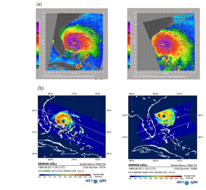
165

Holthuijsen et al. 2012; Vickery et al. 2009; Bell et al. 2012). In this study, the height-resolving,

166

wind-rain interaction model developed by Snaiki and Wu (2017c) (see Appendix A) is utilized.

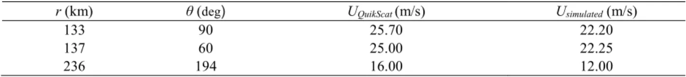
167

Since the rain rate is a necessary input to take the rain effects into account, the iteration technique

168

is employed in the simulation as illustrated by Fig. 2.

9 170

Fig. 2. Flow chart of the rain intensity simulation methodology

171 172

The initial guess of the rain profile could be based on an empirical model as follows (Snaiki and

173 Wu 2017c): 174 0.5 exp 1 b b m m rm r r R R r r          _ _  _ _         (9) 175

where R_rm= maximum rain rate located at the radius of maximum wind r_m; r = radial distance

176

from the tropical cyclone center; and b = scaling parameter that adjusts the profile shape and

177

depends on the radial extent of the tropical cyclone rain field. The maximum rain rate R_rm was

178

estimated with an empirical formula available in literature (Tuleya et al. 2007):

179





1 35 33 rm m R  a b_  V  _ (10) 180

10

where a and b = constants from the least squares fit of the TRMM radial rainfall rates; and V_m=

181

maximum wind speed. Although the iterative calculation is required in the analysis, it converges

182

quite rapidly. With a good initial guess of the rain profile based on Eq. (9), two or three iterations

183

are needed with a prescribed threshold ɛ= 5% for all simulations in the present study. The

first-184

order closure of the rain rate simulation in Fig. 2 results in a simplified model of Eq. (7):

185 wind,modified _wind a m a m r r wind dV dV k k dz dz R V       (11) 186

where k = 100 m_m 2_{/s is the eddy viscosity;}

wind,modified

V = modified wind speed due to the rain effects.

187

In the case of the marine conditions, the effective roughness length z_0,effective could be

188

expressed as a combination of the aerodynamic roughness length z and the rain-induced one ₀ z_0,r

189 (Kumar et al. 2009): 190 0,effective 0 o r, z z z (12) 191

Several formulas have been proposed in the literature to characterize the rain-induced roughness

192

lengthz over ocean. For instance, Kitaigorodskii [referred in Houk and Green (1976)] defined 0,r

193 0,r z as: 194 , 0.03 o r z   (13) 195

where



is the standard deviation of the experimentally obtained mean water level:

196 kD g     (14) 197

11

where  = a constant of 0.01; D = drop diameter; g = gravitational acceleration;



= kinematic

198

viscosity of water; and k is the rain kinetic energy flux that can be related to the rain intensity R

199

and the terminal velocity of the rain drop V : _t

200 2 2 t RV k (15) 201

As a result, the rain-induced roughness can be expressed as:

202 2 0, 0.015 _t r DV R z g





 (16) 203

Accordingly, the rain rate over ocean can be calculated as:

204 2 2 2 10 10 0 0, 0 ln ln a wind r r r z z V z z z R       _{     }  _{     }    _{ }  _{   }     (17) 205

It should be noted that the use of Eq. (17) requires an iteration process since the rain-induced

206

roughness length z depends on the rain intensity._0,r

207

3. Wind field model

208

The proposed analytical framework for rapid estimate of the rain rate requires the horizontal wind

209

speed components as input. A recently developed height-resolving model by Snaiki and Wu

210

(2017a; 2017b) is utilized here due to its high efficiency to obtain the wind field. A brief discussion

211

of the wind field model is presented in this section for the sake of completeness. The governing

212

equation of the wind field is described as follows:

12 1 .   _{       } t _a p f v v v k v F (18) 214

where f = Coriolis parameter; p = pressure; k = unit vector in the vertical direction; and F =

215

frictional force. In order to solve Eq. (18), the decomposition method is used where the wind

216

velocity (v) is expressed as:

217

 g 

v v v' (19)

218

where

v

_g= gradient wind in the free atmosphere; and

v'

= frictional component near the ground

219

surface. The solution of the gradient wind speed could be solved straightforwardly in the

220

cylindrical coordinate system (Georgiou 1986; Meng et al. 1995):

221

















₂ 1/ 2 2 4               _           g a csin fr csin fr _{r p} v r (20) 222

where  = approach angle (counter clockwise positive from the East); c = translation speed of the

223

tropical cyclone; and  = azimuthal angle. The radial velocity

0 1r g rg v dr r v      



obtained from the

224

continuity equation is usually disregarded due to its insignificant effects (Meng et al. 1995).

225

To obtain the frictional wind speed component, the nonlinear governing equation is first

226

simplified using the scale analysis approach, and then linearized leading to the following frictional

227

wind speed formulas as:

228





1/2



( 0 ) (1 ) ( 1 )



0 1 1 ( , ) q z q z i q z i u



z

 

Real A e  A e  A e             (21a) 229



( 0 ) ( 1 ) ( 1 )



0 1 1 ( , ) q z q z i q z i v  z Imag A e  A e  A e            (21b) 230

13

where



u v

', '



= frictional components of the wind velocity; q1   (1 i)   1/2;

231 1/2 1 (1 ) q_   i _    _ ; q0  

 

 1/ 4; 1 2 g m k    ; 1 2 ag m k    ; 2 g g v f r     is the 232

absolute angular velocity; ag g g

v

v

f

r

r

 













is the vertical component of absolute vorticity of the

233 gradient wind;

1

2

g

v

K r







_; 1 2 g v Kr     

 ; and z’= new vertical coordinate used as the base of the

234

computation scheme where z’=0 is located above z (i.e., the 10 m height above the mean height 10

235

of roughness elements) (Meng et al. 1995). The other necessary parameters needed for the

236

simulation can be acquired in Snaiki and Wu (2017a; 2017b).

237

4. Model validation

238

The necessary parameters needed for the tropical cyclone wind field simulation are:



approach

239

angle; c translation velocity of the hurricane; p central pressure; c p central pressure difference;

240

max

R radius of maximum winds; B Holland’s parameter;  latitude; and



longitude. These wind

241

parameters can be obtained from the National Hurricane Center’s North Atlantic Hurricane

242

Database (HURDAT). On the other hand, the tropical cyclone rainfall data can be acquired from

243

the high-fidelity numerical weather prediction models, the Tropical Rainfall Measuring Mission

244

(TRMM) database or the Radar observations.

245

4.1. Comparison with MM5 model

246

In this section, the ensemble average of 12 surface rain fields corresponding to hurricane Frances

247

(2004) in the period from 29th _{August to 1}st _{September 2004 (6-h intervals) were simulated based}

14

on the Fifth-Generation Pennsylvania State University/NCAR Mesoscale Model (MM5)

249

(Langousis and Veneziano 2009a). A resolution of 1.67 km was used to generate the azimuthally

250

averaged rain rates in the MM5 simulations. The rain rates obtained from MM5 were compared

251

with those based on the proposed analytical framework, where the necessary parameters for the

252

rain intensity simulation were extracted from the HURDAT database (Table 1). As shown in Fig.3,

253

a good agreement between the MM5 and present simulation results is achieved.

254

Table 1. Tropical cyclones characteristics of the selected 12 rain fields

255

Hurricane Center

Mon|Day|h Latitude _(deg) Longitude _(deg) Storm Speed _(m/s) Storm Direction _{(deg) (m/s)} Vmax _(hpa) Δp _(km) Rmax

08|29|00 18.1 -52.9 4.0 145 59.2 948 31 08|29|06 18.4 -53.6 3.8 156 59.2 948 31 08|29|12 18.6 -54.4 4.0 165 59.2 948 31 08|29|18 18.8 -55.0 3.5 161 56.6 948 31 08|30|00 18.9 -55.8 3.9 172 54.0 954 32 08|30|06 19.0 -56.8 4.9 174 51.4 958 33 08|30|12 19.2 -58.1 6.4 171 51.4 956 33 08|30|18 19.4 -59.3 5.9 170 56.6 948 31 08|31|00 19.6 -60.7 6.9 171 56.6 946 31 08|31|06 19.8 -62.1 6.9 171 59.2 950 32 08|31|12 20.0 -63.5 6.9 171 61.7 949 32 08|31|18 20.3 -65.0 7.4 168 64.3 942 30 256 257

Fig. 3. Comparison of the azimuthally-averaged, rain-rate radial profile of Hurricane Frances

258 259 0 50 100 150 200 250 300 R (km) 0 5 10 15 20 25 30 35 40 45 50 MM5 simulation Present simulation

15

4.2. Comparison with PR/TRMM rain fields

260

To validate the proposed analysis framework for rapid rain rate estimation during tropical

261

cyclones, 38 PR/TRMM rain frames with a spatial resolution of 5 km5 km were utilized. The

262

parameters of the data collected from the PR/TRMM rain frames are summarized in Table 2

263

(Langousis and Veneziano 2009b). These 38 frames were selected from eight tropical cyclones

264

that cover a wide range of storm intensities. Fig. 4(a) represents a scatterplot of the ratios between

265

the PR/TRMM and simulated rain intensities i_PR /i . A total number of 73819 points were _sim

266

selected from the 38 TRMM frames, covering a wide range of tropical cyclone spatial locations.

267

All the necessary parameters for the rain rate simulation are taken from Table 2 (Langousis and

268

Veneziano 2009b).

269

A large dispersion similar to the finding of Langousis and Veneziano (2009a) is observed in

270

Fig. 4(a). It mainly results from the significant small-scale variability of rain rate due to the

271

rainbands and local intensifications. Figure 4(b) depicts the local average and standard deviation

272

of the ratio i_PR /i with a moving window of 2000 points. Clearly, the simulation based on the _sim

273

proposed analyses framework of rain field is unbiased since the moving average is close to unity.

274

The moving standard deviation on the other hand is quite large highlighting the significance of the

275

small-scale variability of the tropical cyclone rain field (Powell 1990; Molinari et al. 1994;

276

Langousis and Veneziano 2009a).

277

278

279

16 281

Table 2. Tropical cyclones characteristics of the PR/TRMM rain fields (Langousis and Veneziano 2009b)

282 Hurricane Center Hurricane Name Latitude (deg) Longitude (deg) Storm Speed (m/s) Storm Direction (deg) Vmax (m/s) Rmax (km) TRMM Frame Storm Intensity Floyd 1999 21.7 -61.6 4.9 143 48.8 41 10290 CAT2 23.5 -68.7 4.8 169 64.0 37 10317 CAT4 23.7 -70.6 5.8 171 69.3 37 10321 CAT4 Lili 2002 23.6 -87.2 9.0 162 51.5 20 27826 CAT2 24.4 -88.4 6.2 141 56.5 20 27830 CAT2 28.4 -91.4 10.1 117 54.0 20 27842 CAT4 29.0 -91.9 5.4 124 41.1 20 27845 CAT2 Frances 2004 12.6 -43.7 10.9 158 23.1 37 38646 TS 15.7 -49.8 5.4 139 51.4 19 38667 CAT3 17.0 -51.3 5.3 139 54.0 28 38677 CAT3 17.9 -52.6 4.3 144 59.1 28 38682 CAT4 19.0 -57.3 4.9 180 51.4 28 38708 CAT3 21.2 -68.5 6.1 162 61.7 28 38739 CAT4 Ivan 2004 8.9 -38.9 7.6 184 25.7 37 38789 TS 10.7 -50.6 12.2 185 57.5 28 38814 CAT4 11.2 -53.4 8.1 173 51.4 28 38820 CAT3 12.3 -64.1 8.3 166 61.7 19 38845 CAT4 12.7 -66.2 7.3 164 61.7 20 38851 CAT4 17.4 -77.3 4.1 194 66.8 28 38892 CAT4 17.7 -78.4 4.4 153 64.3 28 38897 CAT4 25.6 -87.4 5.5 112 61.7 46 38954 CAT4 Jeanne 2004 27.4 -70.6 5.5 0 38.6 42 39045 CAT1 25.5 -69.5 1.1 207 41.1 37 39079 CAT2 26.5 -74.3 7.4 173 43.7 60 39106 CAT2 26.5 -75.6 6.5 180 46.3 46 39110 CAT2 Karl 2004 11.5 -35.3 7.1 176 26.7 37 38987 TS 17.3 -45.5 2.0 166 57.8 32 39033 CAT3 19.1 -47.4 5.9 121 64.0 32 39048 CAT4 22.9 -48.6 8.2 112 54.0 28 39059 CAT3 25.7 -49.5 6.8 117 48.8 28 39063 CAT3 Katrina 2005 24.6 -85.6 2.1 153 51.5 56 44357 CAT3 25.0 -86.2 3.5 146 56.5 50 44361 CAT3 26.9 -89.0 5.5 135 75.0 38 44373 CAT5 Rita 2005 24.3 -85.9 5.7 189 61.7 28 44743 CAT4 24.9 -88.0 3.9 166 77.1 19 44754 CAT5 25.4 -88.7 4.3 153 72.0 19 44758 CAT5 26.8 -91.0 5.5 135 59.1 37 44770 CAT4 27.4 -91.9 4.8 143 59.1 37 44773 CAT4 283

17 284

Fig. 4. Comparison of the PR/TRMM and simulated rain rates: (a) Scatter plot of i_PR /i_sim; (b) Local average and

285

standard deviation of i_PR/i_sim

286 287

4.3. Comparison with TMI/TRMM and radar observations

288

The rain distribution of hurricane Dennis (1999) obtained from TMI/TRMM (Lonfat et al. 2004)

289

was compared with the simulation result from the present methodology. As shown in Fig. 5, a

290

good agreement between the simulations and observations is highlighted except in some local

291

intensification regions caused by rainbands. TMI measurements are known to be more accurate

292

for rainfall estimates over ocean than land. On the other hand, the Hydro-Next-Generation Doppler

293

Radar system can measure the rainfall distribution over both ocean and land with very good

294

accuracy (Lin et al. 2010). Hurricane Isabel (2003) was employed here to validate rain field

295

simulation over land based on the present analysis framework. Isabel made landfall in North

296

Carolina on 18 September 2003 as a category 2 tropical cyclone and caused widespread damages

297

from storm surge flooding, wind and riverine flooding (Lin et al. 2010). Figure 6 presents a good

298

agreement between the simulated and observed rainfall distribution up to 200 km radius. The

299

orographic enhancement of rainfall due to the interaction between the tropical cyclone and the

18

complex terrain conditions of the central Appalachians Mountains, not considered in the present

301

model, resulted in large differences beyond the range of 200 km (Lin et al. 2010).

302

303

Fig. 5. Comparison of the azimuthally-averaged, rain-rate radial profile of Hurricane Dennis

304 305

306

Fig. 6. Comparison of the azimuthally-averaged, rain-rate radial profile of Hurricane Isabel

307

5. Rainband simulation

308

Tropical cyclones exhibit significant rain rate in the eyewall and a set of rainbands (Willoughby

309

et al. 1984; Willoughby 1988). The complicated underlying mechanisms governing the rainbands

310

make their pattern vary from one tropical cyclone to another (Houze et al. 2006). Hence, it is

311

extremely challenging to systematically simulate these rainbands. The rainbands outside the

312

eyewall are usually characterized by secondary horizontal wind maxima (Samsury and Zipser

313 R ai n ra te ( m m /h )

19

1995). A number of field measurements indicate that the local boundary-layer wind maxima in the

314

rainbands are typically associated with pressure perturbations (e.g., Powell 1990; Yu and Tsai

315

2010; Lin et al. 2010; Sitkowski et al. 2011; Li and Wang 2012). Since the wind field here is

316

simulated by a large-scale model (Snaiki and Wu 2017a; 2017b) and hence does not account for

317

local intensifications, considerable differences between the simulated and observed rain rates are

318

typically observed in the rainband regions as discussed in the preceding sections.

319

A good approach to improve the simulation would be based on a proper perturbation of the

320

original wind profile that could characterize the rainbands. The rain rate heavily depends on the

321

wind speed, hence, a perturbation in the wind field will generate a corresponding perturbation in

322

the rain rate and hence the local maxima of the rain intensity (local perturbation scheme). This

323

approach can be more convenient to be implemented by introducing a perturbation in the pressure

324

profile that will generate a corresponding wind perturbation (Holland et al. 2010). To illustrate the

325

adopted scheme, the rain field of hurricane Dennis (Fig. 5) was revisited to incorporate the

326

contribution of the rainbands. The rainband locations were first identified from the TMI imagery

327

[Fig. 7(b)]. Then, the simulated wind speeds at a 10-meter height were compared with those from

328

the Remote Sensing System QuikScat (version-4) data [Fig. 7(a)] (Ricciardulli and Wentz, 2015)

329

to obtain the perturbation values. Table 3 compares and presents the observed and simulated wind

330

speeds in three different rainband regions. The consideration of perturbations in the wind field

331

leads to an improved rain rate, as shown in Fig. 8. A good agreement between the observed and

332

simulated profiles is observed. Figure 9 presents a comparison of the simulated rain rates of

333

Hurricane Dennis with and without considerations of the rainbands. The corresponding correlation

334

coefficients between the observations and simulations are 0.96 and 0.92, respectively. While the

335

results demonstrate that the rain intensities predicted by both approaches match reasonably well

20

with the measured data, the simulation accuracy is certainly improved by integrating the rainband

337 effects. 338 339 340 341 342 343 344 345 346 347

Fig. 7. Hurricane Dennis (1999) wind and rain fields: (a) Surface wind speed distribution obtained from QuikScat on

348

August 28 (left) and August 29 (right); (b) Surface rain rate provided by TMI/TRMM on August 28 (left) and

349 August 29 (right) 350 351 352 353

21

Table 3. Comparison between the observed (QuikScat) and simulated surface wind speed of Hurricane Dennis in the

354

rainband regions

355

r (km) θ (deg) UQuikScat (m/s) Usimulated (m/s)

133 90 25.70 22.20

137 60 25.00 22.25

236 194 16.00 12.00

356

357

Fig. 8. Comparison of the improved, azimuthally-averaged, rain-rate radial profile of Hurricane Dennis

358

359

360

Fig. 9. Comparison of the azimuthally-averaged rain rates of Hurricane Dennis

361 362 363 100 200 300 400 R (km) 0 2 4 6 8 10 12 14 16

Observed rain rate Simulated rain rate

Si m ul at ed r ai n ra te ( m m /h )

22

6. Sensitivity analysis

364

Numerous studies have demonstrated based on field measurements and numerical simulations that

365

the rainfall distribution varies with a number of environmental factors (e.g., roughness) and

366

inherent tropical cyclone features (e.g., intensity and translation speed) (Lonfat et al, 2004). The

367

present rain rate analysis framework explicitly depends on these parameters. Figure 10 illustrates

368

the sensitivity of the rain intensity to several selected parameters, namely B Holland parameter,

369

m

r radius of maximum wind, c translation speed, p central pressure difference, k turbulent m

370

diffusivity, and z equivalent roughness length. The base case scenario is taken as:0 B1,

371

30

m

r  km,

c



10 /

m s

,  p 70hpa, ₅₀ 2_/

m

k  m s, and z0 0.001m. The radial profile of the

372

rain rate was taken at



 

0

(counterclockwise positive from the East) for all simulations.

373

As indicated in Fig. 10, the central pressure difference



p

, translational tropical cyclone

374

speed c and surface roughness z have significant effects on the rain rate. Actually, it has been ₀

375

widely reported that the surface roughness can substantially alter the rain intensity (e.g., Trenberth

376

et al. 2007; Langousis and Veneziano 2009a; and Lin et al. 2010). Also, a higher value of



p

,

377

corresponding to a larger maximum wind v (Holland et al. 2010), leads to more intense rain. This _m

378

result agrees with the observations and findings of the literature (e.g., Lonfat et al. 2004; Tuleya

379

et al. 2007; Langousis and Veneziano 2009a). Similarly, an increase of the translational tropical

380

cyclone speed results in the enhancement of the total precipitation. Figure 10 also implies that the

381

smaller radius of maximum wind is associated with a more peaked profile shifted to the tropical

382

cyclone center. The Holland’s parameter B mainly modifies the decay rate of the rainfall intensity

383

profile and presents small effects on the maximum rain rate. In addition, low sensitivity of the rain

384

rate to the vertical turbulent diffusivity is noted in the figure.

23 386

Fig. 10. Sensitivity analysis of the rain rate at



 0

387

388

The spatial distribution of the rain intensity was investigated based on the following case

389

study parameters: B = 1.2; c = 3 m/s; rm = 40 km; Δp = 60 hpa; z₀  0.01m. Figures 11(a) and

390

11(b) depict the three-dimensional shaded surface of the rain intensity and their corresponding

391

contours, respectively. Due mainly to the tropical cyclone motion, the rain field is asymmetric.

392

This result conforms with the finding of Langousis and Veneziano (2009a), highlighting the

393

maximum rain rate location near the radius of maximum winds in the eyewall region (Lonfat et al.

394 2004; Tuleya et al. 2007). 395 0 10 20 30 40 50 r_m=30km r_m=40km r_m=50km 0 10 20 30 40 50 B=1 B=1.2 B=1.4 0 10 20 30 40 50 p=50hpa p=70hpa p=90hpa 0 10 20 30 40 50 c=0m/s c=10m/s c=20m/s 100 200 300 r (km) 0 10 20 30 40 50 60 70 z₀=0.001 z₀=0.005 z₀=0.01 100 200 300 r (km) 0 10 20 30 40 50 k_m=40m2/s k_m=50m2/s k_m=60m2/s

24 396

397

Fig. 11. Spatial distribution of the rain rate: (a) Three-dimensional shaded surface of the rain intensity; (b) Contours

398

of the rain rate

399 400

7. Concluding remarks

401

A new, analytical framework for rapid rain rate estimation was proposed in this study. The rain

402

rate formula was essentially developed based on the observation that rain-induced momentum flux

403

at the surface cannot be ignored. The total surface stress results mainly from momentum flux

404

contributions of wind and rain. The obtained results indicate that the spatial distribution of the

405

rainfall field is governed by the wind field inside the tropical cyclone. This observation confirms

406

the findings of several previous studies in which the rain intensity is shown to be highly correlated

407

with the horizontal wind speed. A recently developed, height-resolving wind field model was

408

utilized during the model construction leading to a linear, analytical solution of the surface rain

409

rate. The obtained analysis framework for rain field explicitly depends on parameters for a typical

410

tropical cyclone wind field simulation, namely storm location, approach angle, translation speed,

411

radius of maximum wind, pressure profile, surface drag coefficient, and turbulent diffusivity. The

25

sensitivity analysis was extensively carried out to investigate the effects of several tropical cyclone

413

and environmental parameters on the rain rate. It has been demonstrated that the rain rate heavily

414

depends on the central pressure difference, translational tropical cyclone speed and surface

415

roughness. The proposed analysis framework for the rain field is based on the large-scale

416

horizontal wind field, therefore, it does not account for local rainfall intensifications due to

417

rainbands. A plausible approach based on the local perturbation scheme was introduced to simulate

418

the rain rates inside the rainband regions. The present analytical framework for rapid estimate of

419

rain rate offers good simulation results that are consistent with tropical cyclone observations. It

420

can be readily used in conjunction with the Monte Carlo techniques for risk analysis of tropical

421 cyclone hazards. 422 423 Acknowledgments 424

The support for this project provided by the NSF Grant # CMMI 15-37431 is gratefully

425

acknowledged.

426

427

26

Appendix A

429

The drag force f_i exerted by one raindrop on air in the horizontal direction is introduced:

430 2 , 1 ( ) 2

i  aC Vd r rel rain wind rd

f V V (A.1)

431

where

C

d r, = drag coefficient for a raindrop of radius rd; Vrain= raindrop horizontal velocity; Vwind

432

= wind velocity in the horizontal direction; and V_rel= the total relative speed of the raindrop. As a

433

result, the total drag force f_d applied on a tiny volume of air V  A z can be obtained as follows:

434 , 3 ( ) 4 a d r R C V d    rain wind d V V f (A.2) 435

where d = the raindrop diameter. The total drag force is then integrated into the governing equation

436

of the wind velocity [Eq. (18)]. With several mathematical manipulations, one can obtain the

437

gradient wind speed as follows (Snaiki and Wu 2017c):

438     2 2 2 2 2 1/ 2 2 2 2 2 2 2 2 2 sin 1 2 1 sin 4 1 1 2 ₁                   _  _ _  _                _{      } _{         }       _{  }  _{ }            ag ag g ag ag ag a ag ag c A A f r v A r c A A p A f r r r A r (A.3) 439 where 2 , 1 2 d r d C Nr A  ; and 3 ₃ 4 _d R N r 

 is the number of raindrops per second on a unit area. On

440

the other hand, the frictional wind speed components can be obtained as follows (Snaiki and Wu

441

2017c):

27





' 1cos( ) 2sin( ) az r v Ye W bz W bz (A.4a) 443





' 2cos( ) 1sin( ) az v_ e W bz W bz (A.4b) 444 where Y  p_q ; 1 2 m g p k   ; 1 2 m ag q k   ; 2 , 2 2 d r d NC r

A    . The variables a and b are defined

445 as: 446 2 2 4 2 m m A A _pq k k a  _  _  (A.5a) 447 2 2 4 2 m m A _pq A k k b  _{ }   (A.5b) 448

The variables W1 and W2 are determined form the boundary conditions and presented as follows:

449













1 2 1 rg g a _Z Z _{v Z v} b Y Y W a Z b               _   _   (A.6a) 450

















2 2 1 rg a g Z _{v Z Z v} Y Y b W a _Z b   _{ }           (A.6b) 451 where Cd a, vs kb   ; r r a R Z bk

 



 ; and vs= total wind velocity near the ground surface.

452

Hurricane Katrina (2005) is employed here for the validation purpose. The anemometer

453

was located on the 42003 station at (26°0'25" N, 85°38'54" W). The 10-min averaged time was

28

used for the observed wind data at approximately 10 m height. As shown in Fig. 12, the results

455

generated by the present model are consistent with hurricane Katrina wind field observations.

456

457

458

Fig. 10. Observed and simulated wind speeds (top) and directions (bottom) of Hurricane Katrina 459 460 461 8/27-00Z10 8/27-06Z 8/27-12Z 8/27-18Z 8/28-00Z 8/28-06Z 15 20 25 30 Time (hour) W in d sp ee d (m /s )

Observed wind speed Simulated wind speed

8/27-00Z0 8/27-06Z 8/27-12Z 8/27-18Z 8/28-00Z 8/28-06Z 90 180 270 360 Time (hour) W in d di re ct io n (° )

Observed wind direction Simulated wind direction

29

References

462

Andreas, E.L., 2004. Spray stress revisited. Journal of Physical Oceanography, 34(6), pp.1429-1440.

463

Bryant, K.M. and Akbar, M., 2016. An Exploration of Wind Stress Calculation Techniques in Hurricane Storm Surge

464

Modeling. Journal of Marine Science and Engineering, 4(3), 58.

465

Bell, M.M., Montgomery, M.T. and Emanuel, K.A., 2012. Air–sea enthalpy and momentum exchange at major

466

hurricane wind speeds observed during CBLAST. Journal of the Atmospheric Sciences, 69(11), pp.3197-3222.

467

Caldwell, D.R. and Elliott, W.P., 1971. Surface stresses produced by rainfall. Journal of Physical Oceanography, 1(2),

468

pp.145-148.

469

Caldwell, D.R. and Elliott, W.P., 1972. The effect of rainfall on the wind in the surface layer. Boundary-Layer

470

Meteorology, 3(2), pp.146-151.

471

Chen, S.S., Zhao, W., Donelan, M.A., Price, J.F. and Walsh, E.J., 2007. The CBLAST-Hurricane program and the

472

next-generation fully coupled atmosphere–wave–ocean models for hurricane research and prediction. Bulletin of

473

the American Meteorological Society, 88(3), pp.311-317.

474

Chen, S.S., Zhao, W., Donelan, M.A. and Tolman, H.L., 2013. Directional wind–wave coupling in fully coupled

475

atmosphere–wave–ocean models: Results from CBLAST-Hurricane. Journal of the Atmospheric

476

Sciences, 70(10), pp.3198-3215.

477

Clayson, C.A. and Kantha, L.H., 1999. Turbulent kinetic energy and its dissipation rate in the equatorial mixed

478

layer. Journal of physical oceanography, 29(9), pp.2146-2166.

479

Donelan, M.A., Haus, B.K., Reul, N., Plant, W.J., Stiassnie, M., Graber, H.C., Brown, O.B. and Saltzman, E.S., 2004.

480

On the limiting aerodynamic roughness of the ocean in very strong winds. Geophysical Research Letters, 31(18),

481

L18306.

482

Emanuel, K.A., 1995. Sensitivity of tropical cyclones to surface exchange coefficients and a revised steady-state

483

model incorporating eye dynamics. Journal of the Atmospheric Sciences, 52(22), pp.3969-3976.

484

Fairall, C.W., Kepert, J.D. and Holland, G.J., 1994. The effect of sea spray on surface energy transports over the

485

ocean. Global Atmos. Ocean Syst, 2(2-3), pp.121-142.

486

Fairall, C.W., Bradley, E.F., Rogers, D.P., Edson, J.B. and Young, G.S., 1996. Bulk parameterization of air‐sea fluxes

487

for tropical ocean‐global atmosphere coupled‐ocean atmosphere response experiment. Journal of Geophysical

488

Research: Oceans, 101(C2), pp.3747-3764.

489

Fu, X., Li, H.N. and Yi, T.H., 2015. Research on motion of wind-driven rain and rain load acting on transmission

490

tower. Journal of Wind Engineering and Industrial Aerodynamics, 139, pp.27-36.

491

Garratt, J.R., 1977. Review of drag coefficients over oceans and continents. Monthly weather review, 105(7),

pp.915-492

929.

493

Georgiou, P.N., 1986. Design Wind Speeds in Tropical Cyclone-prone Regions. PhD Thesis University of Western

494

Ontario, London, Ontario, Canada.

495

Groisman, P.Y., Karl, T.R., Easterling, D.R., Knight, R.W., Jamason, P.F., Hennessy, K.J., Suppiah, R., Page, C.M.,

496

Wibig, J., Fortuniak, K. and Razuvaev, V.N., 1999. Changes in the probability of heavy precipitation: important

497

indicators of climatic change. In Weather and Climate Extremes (pp. 243-283). Springer Netherlands.

498

Guo, J.C., Urbonas, B. and Stewart, K., 2001. Rain catch under wind and vegetal cover effects. Journal of Hydrologic

499

Engineering, 6(1), pp.29-33.

30

Holland, G.J., Belanger, J.I. and Fritz, A., 2010. A revised model for radial profiles of hurricane winds. Monthly

501

Weather Review, 138(12), pp.4393-4401.

502

Holthuijsen, L.H., Powell, M.D. and Pietrzak, J.D., 2012. Wind and waves in extreme hurricanes. Journal of

503

Geophysical Research: Oceans, 117, C09003.

504

Houk, D. and Green, T., 1976. A note on surface waves due to rain. Journal of Geophysical Research, 81(24),

pp.4482-505

4484.

506

Houze Jr, R.A., Cetrone, J., Brodzik, S.R., Chen, S.S., Zhao, W., Lee, W.C., Moore, J.A., Stossmeister, G.J., Bell,

507

M.M. and Rogers, R.F., 2006. The hurricane rainband and intensity change experiment: Observations and

508

modeling of Hurricanes Katrina, Ophelia, and Rita. Bulletin of the American Meteorological Society, 87(11),

509

pp.1503-1521.

510

Huang, C.H., 2012. Modification of the Charnock wind stress formula to include the effects of free convection and

511

swell. In Advanced Methods for Practical Applications in Fluid Mechanics. InTech, pp.47-71.

512

Huffman, G.J., Adler, R.F., Bolvin, D.T. and Nelkin, E.J., 2010. The TRMM multi-satellite precipitation analysis

513

(TMPA). In Satellite rainfall applications for surface hydrology (pp. 3-22). Springer Netherlands.

514

Jarosz, E., Mitchell, D.A., Wang, D.W. and Teague, W.J., 2007. Bottom-up determination of air-sea momentum

515

exchange under a major tropical cyclone. Science, 315(5819), pp.1707-1709.

516

Kaplan, J. and DeMaria, M., 1995. A simple empirical model for predicting the decay of tropical cyclone winds after

517

landfall. Journal of applied meteorology, 34(11), pp.2499-2512.

518

Kumar, R.R., Kumar, B.P. and Subrahamanyam, D.B., 2009. Parameterization of rain induced surface roughness and

519

its validation study using a third generation wave model. Ocean Science Journal, 44(3), pp.125-143.

520

Kummerow, C., Barnes, W., Kozu, T., Shiue, J. and Simpson, J., 1998. The tropical rainfall measuring mission

521

(TRMM) sensor package. Journal of atmospheric and oceanic technology, 15(3), pp.809-817.

522

Landsea, C.W., 2000. Climate variability of tropical cyclones: past, present and future. Storms. Routledge, New York,

523

pp.220-241.

524

Langousis, A. and Veneziano, D., 2009a. Theoretical model of rainfall in tropical cyclones for the assessment of long‐

525

term risk. Journal of Geophysical Research: Atmospheres, 114, D02106.

526

Langousis, A. and Veneziano, D., 2009b. Long‐term rainfall risk from tropical cyclones in coastal areas. Water

527

resources research, 45, W11430.

528

Li, Q. and Wang, Y., 2012. Formation and quasi-periodic behavior of outer spiral rainbands in a numerically simulated

529

tropical cyclone. Journal of the Atmospheric Sciences, 69(3), pp.997-1020.

530

Lin, N., Smith, J.A., Villarini, G., Marchok, T.P. and Baeck, M.L., 2010. Modeling extreme rainfall, winds, and surge

531

from Hurricane Isabel (2003). Weather and Forecasting, 25(5), pp.1342-1361.

532

Lonfat, M., Marks Jr, F.D. and Chen, S.S., 2004. Precipitation distribution in tropical cyclones using the Tropical

533

Rainfall Measuring Mission (TRMM) microwave imager: A global perspective. Monthly Weather

534

Review, 132(7), pp.1645-1660.

535

Lonfat, M., Rogers, R., Marchok, T. and Marks Jr, F.D., 2007. A parametric model for predicting hurricane

536

rainfall. Monthly Weather Review, 135(9), pp.3086-3097.

537

Meng, Y., Matsui, M. and Hibi, K., 1995. An analytical model for simulation of the wind field in a typhoon boundary

538

layer. Journal of Wind Engineering and Industrial Aerodynamics, 56(2-3), pp.291-310.

31

Molinari, J., Moore, P.K., Idone, V.P., Henderson, R.W. and Saljoughy, A.B., 1994. Cloud‐to‐ground lightning in

540

Hurricane Andrew. Journal of Geophysical Research: Atmospheres, 99(D8), pp.16665-16676.

541

Powell, M.D., 1990. Boundary layer structure and dynamics in outer hurricane rainbands. Part I: Mesoscale rainfall

542

and kinematic structure. Monthly Weather Review, 118(4), pp.891-917.

543

Powell, M.D., Vickery, P.J. and Reinhold, T.A., 2003. Reduced drag coefficient for high wind speeds in tropical

cy-544

clones. Nature, 422(6929), pp.279-283.

545

Rappaport, E.N., 2000. Loss of life in the United States associated with recent Atlantic tropical cyclones. Bulletin of

546

the American Meteorological Society, 81(9), pp.2065-2073.

547

Ricciardulli, L. and Wentz, F.J., 2015. A scatterometer geophysical model function for climate-quality winds:

548

QuikSCAT Ku-2011. Journal of Atmospheric and Oceanic Technology, 32(10), pp.1829-1846.

549

Samsury, C.E. and Zipser, E.J., 1995. Secondary wind maxima in hurricanes: Airflow and relationship to

550

rainbands. Monthly weather review, 123(12), pp.3502-3517.

551

Shu, Z.R., Li, Q.S., He, Y.C. and Chan, P.W., 2017. Vertical wind profiles for typhoon, monsoon and thunderstorm

552

winds. Journal of Wind Engineering and Industrial Aerodynamics, 168, pp.190-199.

553

Sitkowski, M., Kossin, J.P. and Rozoff, C.M., 2011. Intensity and structure changes during hurricane eyewall

554

replacement cycles. Monthly Weather Review, 139(12), pp.3829-3847.

555

Smith, R.K., 1968. The surface boundary layer of a hurricane. Tellus, 20(3), pp.473-484.

556

Snaiki, R. and Wu, T., 2017a. Modeling tropical cyclone boundary layer: Height-resolving pressure and wind fields.

557

Journal of Wind Engineering and Industrial Aerodynamics, 170, pp.18-27.

558

Snaiki, R. and Wu, T., 2017b. A linear height-resolving wind field model for tropical cyclone boundary layer. Journal

559

of Wind Engineering and Industrial Aerodynamics, 171, pp.248-260.

560

Snaiki, R. and Wu, T., 2017c. Dynamic Interaction of Wind and Rain Fields in the Boundary Layer of a Tropical

561

Cyclone. Proceedings of Engineering Mechanics Institute Conference 2017 (EMI 2017), May, 2017, San Diego,

562

CA, USA.

563

Taylor, G.I., 1916. Skin friction of the wind on the earth's surface. Proceedings of the Royal Society of London. Series

564

A, Containing Papers of a Mathematical and Physical Character, 92(637), pp.196-199.

565

Trenberth, K.E., Davis, C.A. and Fasullo, J., 2007. Water and energy budgets of hurricanes: Case studies of Ivan and

566

Katrina. Journal of Geophysical Research: Atmospheres, 112(D23106).

567

Tse, K.T., Li, S.W., Chan, P.W., Mok, H.Y. and Weerasuriya, A.U., 2013. Wind profile observations in tropical

568

cyclone events using wind-profilers and doppler SODARs. Journal of Wind Engineering and Industrial

569

Aerodynamics, 115, pp.93-103.

570

Tuleya, R.E., DeMaria, M. and Kuligowski, R.J., 2007. Evaluation of GFDL and simple statistical model rainfall

571

forecasts for US landfalling tropical storms. Weather and forecasting, 22(1), pp.56-70.

572

Vickery, P.J., Wadhera, D., Powell, M.D. and Chen, Y., 2009. A hurricane boundary layer and wind field model for

573

use in engineering applications. Journal of Applied Meteorology and Climatology, 48(2), pp.381-405.

574

Willoughby, H.E., Marks Jr, F.D. and Feinberg, R.J., 1984. Stationary and moving convective bands in

575

hurricanes. Journal of the Atmospheric Sciences, 41(22), pp.3189-3211.

576

Willoughby, H.E., 1988. The dynamics of the tropical cyclone core. Australian Meteorological Magazine, 36,

pp.183-577

191.

32

Wilson, P.S. and Toumi, R., 2005. A fundamental probability distribution for heavy rainfall. Geophysical Research

579

Letters, 32, L14812.

580

Wong, B. and Toumi, R., 2016. Effect of extreme ocean precipitation on sea surface elevation and storm

581

surges. Quarterly Journal of the Royal Meteorological Society, 142(699), pp.2541-2550.

582

Woolhiser, D.A. and Roldan, J., 1982. Stochastic daily precipitation models: 2. A comparison of distributions of

583

amounts. Water resources research, 18(5), pp.1461-1468.

584

Wu, J., 1973. Spray in the atmospheric surface layer: Laboratory study. Journal of Geophysical Research, 78(3),

585

pp.511-519.

586

Yu, C.K. and Tsai, C.L., 2010. Surface pressure features of landfalling typhoon rainbands and their possible

587

causes. Journal of the Atmospheric Sciences, 67(9), pp.2893-2911.

588

Zhao, D., Ma, X., Liu, B. and Xie, L., 2013. Rainfall effect on wind waves and the turbulence beneath air-sea interface.

589

Acta Oceanologica Sinica, 32(11), pp.10-20.