is an open access repository that collects the work of Arts et Métiers Institute of
Technology researchers and makes it freely available over the web where possible.
This is an author-deposited version published in: https://sam.ensam.eu
Handle ID: .http://hdl.handle.net/10985/18181
To cite this version :
Marc RÉBILLAT, Nazih MECHBAL - Damage localization in geometrically complex aeronautic structures using canonical polyadic decomposition of Lamb wave difference signal tensors -Structural Health Monitoring - Vol. 19, n°1, p.305-321 - 2020
canonical polyadic decomposition of Lamb wave difference signal tensors
Marc Rébillat & Nazih Mechbal*
*PIMM Laboratory, Ensam, CNRS, Cnam, Hesam Université, Paris, France (e-mail: [email protected] – [email protected] ).
Abstract: Monitoring in real time and autonomously the health state of aeronautic structures is referred to as Structural
Health Monitoring (SHM) and is a process decomposed in four steps: damage detection, localization, classification, and quantification. In this work, the structures under study are aeronautic geometrically complex structures equipped with a bonded piezoelectric network. When interrogating such a structure, the resulting data lie along three dimensions (namely the “actuator, “sensor”, and “time” dimensions) and can thus be interpreted as three-way tensors. The fact that Lamb wave SHM based data are naturally three-way tensors is here investigated for damage localization purpose. In this paper it is demonstrated that under classical assumptions regarding wave propagation, the canonical polyadic decomposition of rank 2 of the tensors build from the phase and amplitude of the difference signals between a healthy and damaged states provide direct access to the distances between the piezoelectric elements and damage. This property is used here to propose an original tensor-based damage localization algorithm. This algorithm is successfully validated on experimental data coming from a scale one part of an airplane nacelle (1.5 m in height for a semi circumference of 4 m) equipped with 30 piezoelectric elements and many stiffeners. Obtained results demonstrate that the tensor-based localization algorithm can locate a damage within this structure with an average precision of 10 cm and with a precision lower than 1 cm at best. In comparison with standard damage localization algorithms (delay-and-sum, RAPID, and ellipse- or hyperbola-based algorithms) the proposed algorithm appears as more precise and robust on the investigated cases. Furthermore, it is important to notice that this algorithm only takes the raw signals as inputs and that no specific pre-processing steps or finely tuned external parameters are needed. This algorithm is thus very appealing as reliable and easy to settle damage localization timeliness with low false alarm rates are one of the key successes to shorten the gap between research and industrial deployment of SHM processes.
Keywords: structural health monitoring, damage localization, tensors, canonical polyadic decomposition, lamb waves, piezoelectric elements
1. INTRODUCTION
Monitoring in real time and autonomously the health state of structures is of high interest in the industry, and more specifically in the aeronautic and civil engineering application fields. Such a process is referred to as Structural Health Monitoring (SHM) [1, 2]. To achieve this goal, structures become “smart” in the sense that they are equipped with sensors, actuators, and artificial intelligence that allow them to state autonomously regarding their own health. One can compare smart structures with the human body which, thanks to its various senses and nerves, is able to assess if it has been hurt, where it has been hurt, and to estimate how severe it is. Following this analogy, the SHM process is classically decomposed into four steps: damage detection, localization, classification, and quantification [3].
Structures under study are here geometrically complex aeronautics structures. To perform damage monitoring of such structures, a variety of techniques have been developed [1, 4]. Evaluation of Lamb wave propagation based on an interrogation scheme bonded on structures is one of the most successful techniques. To deploy Lamb wave based SHM to such structures, they are equipped with piezoelectric elements that can be used both as sensors and actuators. A piezoelectric actuator emits periodic bursts, exciting Lamb waves within the structure, and a set of receiving sensors generate output signals (in a so-called “pitch-catch” approach) that are then processed in order to extract structure condition and damage related information [5, 6, 7, 8]. Lamb wave-based damage localization in structures relies on the fundamental idea that damage causes signal scattering. When a propagating wave in a solid medium interacts with any structural discontinuity, the wave reflects in various directions, depending on the discontinuity shape. The scattered signal is obtained using baseline subtraction from the current signal. However, in the case of complex structures, induced wave dispersion and mode conversion due to interaction with structural discontinuities or boundaries, make reliable damage localization a challenging task.
Considering a smart structure equipped with 𝑁 piezoelectric elements and for which acquisition is performed over 𝐾 samples, one naturally ends up with a matrix 𝑴 ∈ ℝ𝑁×𝑁×𝐾 at the end of a pitch-catch SHM process. To monitor the possible apparition of damage, measurements are first performed in a reference state to get a reference matrix 𝑹. Then, during the life cycle of the structure, measurements at unknown states are performed and provides the matrix 𝑼. The matrix 𝛅 that corresponds
to the difference between 𝑹 and 𝑼 is the basis of the detection, localization, classification, and quantification steps of SHM. Many SHM algorithms have been tested and validated on simple plates but their application to geometrically complex aeronautics structures remains a challenge [9].When interrogating a smart structure equipped with a bonded piezoelectric network, the resulting difference matrix 𝜹 ∈ ℝ𝑁×𝑁×𝐾lie along three dimensions (namely the “actuator, “sensor”, and “time” dimensions) and can thus be interpreted as three-way tensors [10, 11, 12]. Even if during the last decade, tensors have been widely applied for signal processing purposes [10, 11, 12], they have found relatively few applications in SHM and reported applications mainly focused on the detection step. For example: damage detection based on tensors in a civil engineering context [13, 14], tensor-based damage detection for non-destructive evaluation of composite structures using ultrasounds [15], or application of tensors for denoising purposes in composite plates monitored by ultrasonic waves [16]. Thus, to the knowledge of the authors, the potential of tensors for damage localization by means of Lamb waves in composite plates has never been investigated.
The focus is specifically put in this paper on the localization step of the SHM process. Existing methods relying on Lamb waves can be divided in several classes [17, 7, 6, 5]. The first class of localization method, “time” methods, use the time information related to the scattered signal for a given actuator sensor path to draw ellipses or hyperbola that should intersect at the damage position [18, 19, 20, 21, 22, 23, 24]. Some attempts to use the amplitude of the scattered signals are also reported in the literature [25, 26] leading to the “amplitude” class of methods. Another class of methods, called “delay and sum”, sums over all possible paths the scattered signal delayed as if it originates from a given position in order to infer the probability that the damage is present at that position [27, 28, 29, 30, 31, 32]. Extending that idea, methods termed “correlation” rely on physical models of waves propagation. Using such models, the scattered signals are computed for each path and for different potential damage positions. The position at which the correlation between the model and actual scattered signals is maximal then indicates the most likely damage position [33, 34, 35, 36, 37, 38]. More recently, some methods referred to as “sparse”, try to infer from a physical model, the structure of the global difference matrix containing all the scattered signals and solve an optimization problem in order to estimate damage location [39, 40]. Classical methods for damage localization by mean of Lamb waves in composite plates (respectively “time”, “amplitude”, “delay and sum” and “correlation”) are thus based on a path by path analysis of data (i.e. only one row of the matrix 𝜹 ∈ ℝ𝑁×𝑁×𝐾 is used at first). These methods thus process each path independently
and then integrate empirically all the information together to form a localization map from which damage localization is inferred. The classical way of addressing damage localization through Lamb waves consists indeed in trying to model as accurately as possible the wave propagation within the structure under study. However, such an intuitive approach cannot be robust in practice given the complexity and variability of structures at hand and has not been retained here.
As SHM data are three-way, highly redundant, and correlated, a vector-based one-way approach as depicted above cannot capture all these relationships and correlations together. The class of “sparse” methods appears as a first attempt to do so [39, 40]. Tensors naturally appear as an alternate tool able to manage SHM data all at once without processing data path by path, which is one of the major drawbacks of traditional approaches. Tensor-based method, under the assumption that collected data can be partially described by a minimal model of Lamb wave propagation, can rely on this model as a structuring basis for data analysis. Adequate and unified data analysis (in opposition to previously mentioned “path by path” analysis) could then allow to highlight the underlying structure of SHM data and thus potentially to estimate damage location. Indeed, in an industrial context a high efficiency MRO (Maintenance, Repair and Overhaul) process monitored by SHM algorithms is needed (especially in the aeronautical industry). Damage localisation timeliness reliable, easy to settle, and with low false alarm are thus one of the key successes to shorten the gap between research and industrial deployment of SHM processes [9].
The aim of this paper is thus to demonstrate that under classical assumptions regarding wave propagation, the decomposition of tensors build from the difference signals between a healthy and damaged states provides direct access to the distances between the piezoelectric elements and damage and can thus be used to design an original damage localization algorithm. Challenging experimental data coming from a scale one part of an airplane nacelle (1.5 m in height for a semi circumference of 4 m) equipped with 30 piezoelectric elements and many stiffeners will be used for this study. The paper is organized as follows: a tensor-based damage localization algorithm is detailed in Sec. 2 and then validated experimentally and compared to standard damage localization algorithms from the literature in Sec.3. A conclusion and a discussion are then drawn in Sec. 4 and Sec. 5.
2. TENSOR-BASED DAMAGE LOCALIZATION
2.1 An intuitive physical model of Lamb wave propagation
Wave propagation within thin plates structures can be as a first approximation, thought intuitively as follows: waves propagate with a velocity 𝑣 in all directions around their excitation point and are attenuated with an exponential decay 𝛼(𝑑) = exp(−𝜅𝑑) where 𝜅 is a global attenuation parameter [41, 42, 43, 44]. Then, in the absence of damage, a wave 𝑠(𝑡) is sent by the piezoelectric element 𝑛 and the other elements {𝑚 ∈ 1: 𝑁, 𝑚 ≠ 𝑛} receive the signals:
𝑠𝑛𝑚𝑅 (𝑡) = 𝑒𝑥𝑝(−𝜅𝑑𝑛𝑚)𝑠 (𝑡 −
𝑑𝑛𝑚𝑓𝑠
𝑣 ) Eq. 1
where 𝑑𝑛𝑚 denotes the distance between the elements 𝑛 and 𝑚, 𝑡 the sampled time and 𝑓𝑠 the sampling frequency. It is important
to notice here that isotropy is assumed whereas it may not be perfectly the case in practice.
Let’s now introduce a damage at position 𝐷 within this structure. When the wave emitted by the element 𝑛 hits the damage, it is reflected, and a new wave is reemitted within the structure. As a first approximation, one can assume that damage acts as a
secondary wave source that reemits any incoming wave in all directions with a reflection coefficient 𝛽 ∈ ℝ+ [7]. The signal
received by the element 𝑚 is then:
𝑠𝑛𝑚𝑈 (𝑡) = 𝑠𝑛𝑚𝑅 (𝑡) + 𝛽𝑒𝑥𝑝(−𝜅𝑑𝑛𝐷)𝑒𝑥𝑝(−𝜅𝑑𝐷𝑚)𝑠 (𝑡 −
𝑓𝑠(𝑑𝑛𝐷+ 𝑑𝐷𝑚)
𝑣 ) Eq. 2
If the focus is now put on the difference signal, 𝛿𝑛𝑚(𝑡), one has:
𝛿𝑛𝑚(𝑡) = 𝑠𝑛𝑚𝑈 (𝑡) − 𝑠𝑛𝑚𝑅 (𝑡) = 𝛽𝑒𝑥𝑝(−𝜅(𝑑𝐷𝑚+𝑑𝑛𝐷))𝑠 (𝑡 −
𝑓𝑠(𝑑𝑛𝐷+ 𝑑𝐷𝑚)
𝑣 ) Eq. 3
It is then possible to take the Fourier transform of this signal and one ends up with the following transfer function:
𝐻𝑛𝑚𝑘 =
Δ𝑛𝑚(𝑘)
𝑆(𝑘) = 𝛽𝑒𝑥𝑝(−𝜅(𝑑𝑛𝐷+ 𝑑𝐷𝑚))𝑒𝑥𝑝 (−𝑖2𝜋𝑓𝑠𝑘 (
𝑑𝑛𝐷+ 𝑑𝐷𝑚
𝐾𝑣 )) Eq. 4
where 𝑆(𝑘) denotes the Fourier transform of the input signal 𝑠(𝑡), Δ𝑛𝑚(𝑘) the Fourier transform of the difference signal 𝛿𝑛𝑚(𝑡),
𝑘 the current frequency index, and 𝐾 the total number of samples. 𝐻𝑛𝑚𝑘 is thus the 𝑘-th coefficient of the discrete Fourier
transform of the transfer function linking the difference signal on the path “actuator 𝑛 – sensor 𝑚” with the input signal. It is then possible to compute the phase and amplitude of each element 𝐻𝑛𝑚𝑘:
Φ𝑛𝑚𝑘= 𝜙[H𝑛𝑚𝑘] = −𝑖2𝜋𝑓𝑠𝑘 (
𝑑𝑛𝐷+ 𝑑𝐷𝑚
𝐾𝜈 ) Eq. 5
𝐴𝑛𝑚𝑘= log[H𝑛𝑚𝑘] = log 𝛽 − 𝜅(𝑑𝑛𝐷+ 𝑑𝐷𝑚) Eq. 6
The matrices 𝚽 ∈ ℝ𝑁×𝑁×𝐾 containing the coefficients Φ
𝑛𝑚𝑘 and 𝐀 ∈ ℝ𝑁×𝑁×𝐾 containing the coefficients A𝑛𝑚𝑘 can then be
naturally interpreted as three-way tensors [10, 11, 12].
2.2 Canonical polyadic decomposition of the phase tensor
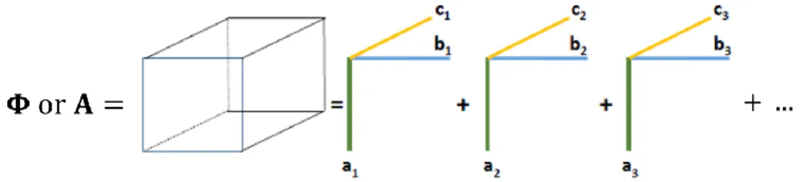
The idea is now to be able to make an interesting structure popping out of the tensors 𝚽 and 𝐀 defined in Eq. 5 and Eq. 6. From tensors literature, it is well known that tensors can be decomposed using the Canonical Polyadic Decomposition (CPD) up to a rank 𝑅 [10, 11, 12]. Such decomposition consists in finding a triplet (𝒂 ∈ ℝ𝑁×𝑅, 𝒃 ∈ ℝ𝑁×𝑅, 𝒄 ∈ ℝ𝐾×𝑅) that allows for a more compact representation of a given tensor (see Fig. 1).
Fig. 1: Schematic representation of the CPD of tensors 𝚽 and 𝑨
According to the notations of Fig. 1, the CPD of the phase tensor 𝚽 defined in Eq. 5 can be expressed as: Φ𝑛𝑚𝑘 = ∑ 𝑎𝑟𝑛Φ𝑏𝑟𝑚Φ
𝑅
𝑟=1
𝑐𝑟𝑘ΦΦ𝑛𝑚𝑘 Eq. 7
What is interesting here is that by analyzing Eq. 5, the tensor 𝚽 can be exactly expressed as a tensor of rank 𝑅 = 2 by choosing: 𝒂𝚽= [𝑑…1𝐷 …1 𝑑𝑁𝐷 1 ] 𝒃𝚽= […1 𝑑…1𝐷 1 𝑑𝑁𝐷 ] 𝒄𝚽=2𝜋𝑓𝑠 𝐾𝑐 [ 0 0 … … (𝑘𝑀− 𝑘0) (𝑘𝑀− 𝑘0) ] Eq. 8 where 𝑘0 and 𝑘𝑀stands for the frequency indexes over which the phase analysis starts and stops.
Furthermore, when removing the constant offset log 𝛽, the CPD of the amplitude tensor 𝑨 whose elements are defined in Eq. 6 can be expressed as:
𝐴̃𝑛𝑚𝑘= 𝐴𝑛𝑚𝑘− log 𝛽 = ∑ 𝑎𝑟𝑛A 𝑏𝑟𝑚A 𝑅
𝑟=1
𝑐𝑟𝑘AΦ𝑛𝑚𝑘 Eq. 9
𝒂𝑨= [𝑑…1𝐷 …1 𝑑𝑁𝐷 1 ] 𝒃𝑨= […1 𝑑…1𝐷 1 𝑑𝑁𝐷 ] 𝒄𝐴= −𝜅 [… …1 1 1 1 ] Eq. 10
By looking in more detail at this tensor decomposition, it is particularly striking to notice that 𝒂𝚽, 𝒂𝑨, 𝒃𝚽 and 𝒃𝑨 all provide
direct access to {𝑑𝑖𝐷}𝑖∈[1,𝑁] that are the distances between each piezoelectric element and the damage position. On the knowledge
of these distances, damage localization is thus theoretically possible. Furthermore, 𝒄𝚽 is parametrized by 𝑣 the wave velocity
within the material and by the signal processing parameters 𝑓𝑠 and 𝐾, and 𝒄𝐀 is parametrized only by 𝜅 the attenuation coefficient.
All these parameters are relatively easy to estimate in practice.
In summary, it is demonstrated here that the CPDs of rank 𝑅 = 2 of the phase and amplitudes of the difference signals between a healthy and damaged states potentially provides direct access to all the distances between the piezoelectric elements and the damage, which could allow for damage localization.
2.3 Managing unicity of CPD
Unfortunately, even if very efficient numerical tools are available to compute a CPD for a given tensor [45], such decomposition is not unique. The issue is that here not only a decomposition is sought, but a decomposition that can be physically interpreted according to Eq. 8 and Eq. 10. Therefore, a way to descale the numerically obtained CPDs, or to obtain a unique one that makes sense physically is needed.
Mathematically, for the phase tensor 𝚽, once a first decomposition (𝒂̃𝚽, 𝒃̃𝚽, 𝒄̃𝚽) has been numerically obtained, what is
needed is to find the descaling coefficients {𝜆𝐴1, 𝜆𝐴2, 𝜆𝐵1, 𝜆𝐵2, 𝜆𝐶1, 𝜆𝐶2} such that:
𝒂𝚽= [𝑑…1𝐷 …1 𝑑𝑁𝐷 1 ] = 𝒂̃𝚽[𝜆𝐴1 0 0 𝜆𝐴2] = [ 𝛼1 𝜉 … … 𝛼𝑁 𝜉 ] [𝜆𝐴1 0 0 𝜆𝐴2] Eq. 11 𝒃𝚽= […1 𝑑…1𝐷 1 𝑑𝑁𝐷 ] = 𝒃̃𝚽[𝜆𝐵1 0 0 𝜆𝐵2] = [ 𝛾 𝛿1 … … 𝛾 𝛿𝑁 ] [𝜆𝐵1 0 0 𝜆𝐵2] Eq. 12 𝒄𝚽= 2𝜋𝑓𝑠 𝑣𝐾 [ 0 0 … … 𝑘𝑚− 𝑘0 𝑘𝑚− 𝑘0 ] = 𝒄̃𝚽[𝜆𝐶1 0 0 𝜆𝐶2] = [ 𝜇1 𝜖1 … … 𝜇𝐾 𝜖𝐾 ] [𝜆0𝐶1 𝜆0 𝐶2] Eq. 13
satisfying the following constraints [11]:
{𝜆𝜆𝐴1𝜆𝐵1𝜆𝐶1 = 1
𝐴2𝜆𝐵2𝜆𝐶2 = 1 Eq. 14
By now analyzing the above equations, it can be easily seen that these coefficients can be estimated as: 𝜆𝐴2= 1/𝜉 𝜆𝐶1 = 𝑚𝑒𝑎𝑛 [ 2𝜋𝑓𝑠(𝑘 − 𝑘0) 𝐾𝑣𝜇𝑘 ] 𝜆𝐴1= 1 𝜆𝐵1𝜆𝐶1 𝜆𝐵1= 1/𝛾 𝜆𝐶2 = 𝑚𝑒𝑎𝑛 [ 2𝜋𝑓𝑠(𝑘 − 𝑘0) 𝐾𝑣𝜖𝑘 ] 𝜆𝐵2= 1 𝜆𝐴2𝜆𝐶2 Eq. 15
For the amplitude matrix 𝑨, once a first decomposition (𝒂̃𝑨, 𝒃̃𝑨, 𝒄̃𝑨) what is needed is to find the descaling coefficients
{𝜁𝐴1, 𝜁𝐴2, 𝜁𝐵1, 𝜁𝐵2, 𝜁𝐶1, 𝜁𝐶2} such that: 𝒂𝑨= [𝑑…1𝐷 …1 𝑑𝑁𝐷 1 ] = 𝒂̃𝑨[𝜁𝐴1 0 0 𝜁𝐴2] = [ 𝛼1 𝜉 … … 𝛼𝑁 𝜉 ] × [𝜁𝐴1 0 0 𝜁𝐴2] Eq. 16 𝒃𝑨= […1 𝑑…1𝐷 1 𝑑𝑁𝐷 ] = 𝒃̃𝑨[𝜁𝐵1 0 0 𝜁𝐵2] = [ 𝛾 𝛿1 … … 𝛾 𝛿𝑁 ] × [𝜁𝐵1 0 0 𝜁𝐵2] Eq. 17 𝒄𝑨= −𝜅 [… …1 1 1 1] = 𝒄̃ 𝑨[𝜁𝐶1 0 0 𝜁𝐶2] = [ 𝜇1 𝜖1 … … 𝜇𝑘𝑚𝑎𝑥 𝜖𝑘𝑚𝑎𝑥] × [ 𝜁𝐶1 0 0 𝜁𝐶2] Eq. 18
satisfying the following constraints [11]:
{𝜁𝜁𝐴1𝜁𝐵1𝜁𝐶1 = 1
𝐴2𝜁𝐵2𝜁𝐶2 = 1 Eq. 19
𝜁𝐴2= 1/𝜉 𝜁𝐶1 = 𝑚𝑒𝑎𝑛 [ −𝜅 𝜇𝑘] 𝜁𝐴1= 1 𝜁𝐵1𝜁𝐶1 𝜁𝐵1= 1/𝛾 𝜁𝐶2 = 𝑚𝑒𝑎𝑛 [ −𝜅 𝜖𝑘] 𝜁𝐵2= 1 𝜁𝐴2𝜁𝐶2 Eq. 20
It is important here to notice that to go back from an arbitrary numerical CPD to a CPD that is physically relevant, the knowledge of the velocity 𝑣 and of the attenuation coefficient 𝜅 are needed. These descaling factors, i.e. the velocity and attenuation of Lamb waves within the material, are here necessary to convert a time-domain information (extracted from phase) and a level information (extracted from amplitude) to a distance information as done in any classical localization algorithm [24, 46, 7]. It is worth mentioning here that these parameters can be very easily estimated from experimental data in the reference state by computing the times and levels of arrivals of the first wave packets and making use of the known distances between piezoelectric elements.
In summary, it is shown here that starting from a numerical CPD of the phase tensor and using knowledge on the velocity 𝑣 and attenuation 𝜅 of Lamb waves within the material under study derived from input experimental data, it is possible to access to four estimates of the distances between all the piezoelectric elements and the damage that are denoted in the following as: {𝑑𝑖𝐷Φ𝑎}𝑖∈[1,𝑁], {𝑑𝑖𝐷Φ𝑏}𝑖∈[1,𝑁], {𝑑𝑖𝐷A𝑎}𝑖∈[1,𝑁] and {𝑑𝑖𝐷A𝑏}𝑖∈[1,𝑁]. Even if theoretically ∀𝑖 ∈ [1, 𝑁]𝑑𝑖𝐷𝛷𝑎= 𝑑𝑖𝐷𝛷𝑏 = 𝑑𝑖𝐷𝐴𝑎= 𝑑𝑖𝐷𝐴𝑏, this may not
be the case in practice due to several factors (experimental noise, numerical issues, …) and it has thus been chosen to introduce and to keep the four notations.
2.4 Damage localization imaging
The last step of the damage localization algorithm consists now in drawing a map able to highlight the most probable damage localization from some or all of the four sets of distances {𝑑𝑖𝐷Φ𝑎}𝑖∈[1,𝑁], {𝑑𝑖𝐷Φ𝑏}𝑖∈[1,𝑁], {𝑑𝑖𝐷A𝑎}𝑖∈[1,𝑁] and {𝑑𝑖𝐷A𝑏}𝑖∈[1,𝑁] estimated previously. Let’s consider a structure under study over which coordinates of a current point 𝑀 can be defined. It is then possible to compute for any current point on the structure the distances {𝑑𝑖𝑃}𝑖∈[1,𝑁] between this current point and the 𝑁 piezoelectric
elements. The point of the structure that will most probably be the damage location should in theory satisfyfor any𝑖 ∈ [1, 𝑁]: 𝑑𝑖𝑃 = 𝑑𝑖𝐷Φ𝑎= 𝑑𝑖𝐷Φ𝑏 = 𝑑𝑖𝐷A𝑎= 𝑑𝑖𝐷A𝑏 Eq. 21
Therefore, three intuitive damage localization indexes relying on the distances estimated from the phase tensor P(𝑀), the amplitude tensor A(𝑀), or both tensors PA(𝑀) can be defined as:
P(𝑀) = 1 ∑𝑁𝑖=1(2𝑑𝑖𝑃− 𝑑𝑖𝐷Φ𝑎− 𝑑𝑖𝐷Φ𝑏)2 Eq. 22 A(𝑀) = 1 ∑𝑁𝑖=1(2𝑑𝑖𝑃− 𝑑𝑖𝐷𝐴𝑎− 𝑑𝑖𝐷𝐴𝑏)2 Eq. 23 PA(𝑀) = 1 ∑𝑁𝑖=1(4𝑑𝑖𝑃− 𝑑𝑖𝐷Φ𝑎− 𝑑𝑖𝐷Φ𝑏− 𝑑𝑖𝐷𝐴𝑎− 𝑑𝑖𝐷𝐴𝑏)2 Eq. 24
Finally, the damage imaging algorithm simply consists of plotting P(𝑀), A(𝑀), or PA(𝑀) over the structure under study and in searching for its maximum value.
2.5 Algorithm overview
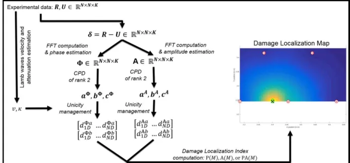
An overview of the proposed damage localization algorithm is provided in Fig. 2. This algorithm can be summarized as follows: - Step 1: Compute the difference matrix 𝜹 between a reference and an unknown state.
- Step 2: Compute the phase and amplitude of the Fourier transform for the difference signal on the path “actuator 𝑛 – sensor 𝑚” and build the tensors 𝚽 and 𝑨 on this basis (see Sec. 2.1).
- Step 3: Compute the CPD of rank 𝑅 = 2 of the tensors 𝚽 and 𝑨 (see Sec. 2.2).
- Step 4: Estimate Lamb wave velocity 𝑣 and attenuation 𝜅 and use them to descale the previous numerically obtained CPDs and extract damage to piezoelectric elements distances estimates {𝑑𝑖𝐷Φ𝑎}
𝑖∈[1,𝑁], {𝑑𝑖𝐷 Φ𝑏}
𝑖∈[1,𝑁], {𝑑𝑖𝐷 A𝑎}
𝑖∈[1,𝑁] and
{𝑑𝑖𝐷A𝑏}𝑖∈[1,𝑁] (see Sec. 2.3).
- Step 5: Compute a damage localization index chosen among P(𝑀), A(𝑀), or PA(𝑀) and draw a damage localization map in order to estimate the most probable damage localization (see Sec. 2.4).
It is of primary importance to notice here that no tuning parameters or specific pre-processing steps are needed for this algorithm to run. The input data are directly fed to the algorithm which processes them without the need of any external parameter or path selection algorithm. Furthermore, the attenuation coefficient κ and the wave velocity ν can be estimated in practice using
data in the healthy state. For a given path in the healthy state, the time of arrival of the first wave packet and the knowledge of the distance between the actuator and the sensor can provide an estimate of the wave velocity ν. For two given paths with the same actuator in the healthy state, the maximum amplitudes of both wave packets as well as the distances between the actuator and the sensors, under the assumption of an exponential spatial decay and isotropy, can allow for the estimation of the attenuation coefficient κ.
Fig. 2: Overview of the damage localization algorithm 3. EXPERIMENTAL RESULTS
This section describes an experimental validation of the tensor-based damage localization algorithm proposed in Sec. 2 on a full-scale geometrically complex aeronautics structure as well as a quantitative comparison of the proposed algorithm with standard damage localization algorithms from the literature.
3.1 Experimental setup
The geometrically complex aeronautics structure under study consists here in the fan cowl part of a nacelle of an Airbus A380. This structure is 1.5 m in height for a semi circumference of 4 m and is made of composite monolithic carbon epoxy material. It has been equipped with 30 piezoelectric elements manufactured by NOLIAC (diameter of 25 mm) and possesses many stiffeners delimiting various areas; as shown in Fig.3. To illustrate the tensor-based localisation algorithm, this structure has been divided in four subparts delimited by the stiffeners on which the localization algorithm performances will be evaluated: - HOLE: this subpart is depicted in green in Fig.3 and has been selected because there is a hole between the piezoelectric
elements 12, 15 and 16. This complex geometrical configuration is a challenging issue for any damage localization algorithm. On this structure, the damage has been simulated using two 35 mm Neodymium magnets placed on both faces of the structure at the position indicated by the green “×”. An excitation frequency of 𝑓0= 200 𝑘𝐻𝑧 has been
used for this subpart.
- SIDE: this subpart is depicted in yellow on Fig.3 and has been selected because it is close to an academic case with no
real specificities. The influence of excitation frequency will be investigated in this area excitation and frequencies of 𝑓0= 150 𝑘𝐻𝑧 and 𝑓0= 200 𝑘𝐻𝑧 have been used. Damage is again simulated using two 35 mm Neodymium magnets
placed on both faces of the structure at the position indicated by the yellow “×”.
- CENTER: this subpart is depicted in red in Fig.3. This subpart is larger than the other subparts (4 m long) with a very
large aspect ratio. It also constitutes a challenging case for the localization algorithm. The damage is simulated using two 35 mm Neodymium magnets placed on both faces of the structure at the position indicated by the red “×”. An excitation frequency of 𝑓0= 200 𝑘𝐻𝑧 has been used in this subpart.
- FULL: this appellation gathers all the previously defined subparts. This part contains all the 30 piezoelectric elements
and is particularly challenging because it contains several stiffeners. The damage is simulated using two 35 mm Neodymium magnets placed on both faces of the structure at the position indicated by the yellow “×”, as in the “SIDE” case. An excitation frequency of 𝑓0= 200 𝑘𝐻𝑧 has been used in this subpart.
Fig.3: Fan cowl of an A380 Nacelle made of composite materials and equipped with 30 piezoelectric elements and possessing many stiffeners. The various areas under study as well as the corresponding damage positions are indicated with different colors.
The excitation signal sent to the PZT element is a “5 cycles burst” with an excitation frequency of 𝑓0= 150 𝑘𝐻𝑧 or 𝑓0=
200 𝑘𝐻𝑧 (see above) and with an amplitude of 10 V. The excitation frequency is usually selected to promote one propagation mode over another. Typically, the mode 𝑆0 is promoted over the mode 𝐴0 as it propagates faster. This is what has been done
here by selecting two frequencies for which this mode is dominant with the experimental setup at hand [7, 24, 47]. The Lamb wave propagation speed within the material is estimated around 5200 m/s for the 𝑆0 mode. In each phase of the experimental
procedure, one PZT is selected as the actuator and the other act as sensors. All the PZTs act sequentially as actuators. Resulting signals are then simultaneously recorded by the other piezoelectric elements and consist of 1500 data points sampled at 1𝑀𝐻𝑧. Signals were acquired 10 times in both the healthy (reference) and damaged (unknown) states.
As pre-processing steps, the measured signals are first denoised by means of a discrete wavelet transform up to the order 4 using the “db40” wavelet. Those signals are then filtered around their excitation frequency 𝑓0 using a continuous wavelet
transformation based on “morlet” wavelets and with a scale resolution equal to 20. The objective of this pre-processing step is to perform a band pass filtering around the excitation frequency 𝑓0 by means of wavelets. The scale parameter can be sought as an image of the bandwidth of the retained bandpass filter over the frequency range of interest. Here, choosing it equal to 20 is something relatively common as it provides convenient results in past studies [7, 24, 47]. In those studies, an optimization algorithm based on the Shannon entropy was applied to select the best wavelet family as well as the best scale parameters to maximize the information contained within the wavelet decomposition. The diaphonic part present in the measured signals (i.e. the copy of the input signals that appears on the measured signal due to electromagnetic couplings in wires) has been previously eliminated based on the knowledge of the geometrical positions of the PZT and of the estimated waves propagation speed 𝑣 in the material.
3.2 CPD of the phase tensor in practice
To build the tensors 𝚽 and 𝑨 (see Sec. 2.1), the matrix 𝜹 containing the differences of signals between the healthy and damaged states have been built. To remove undesirable reflections from the difference signals, only the first wave packets have been retained in the difference signals. In Fig. 4 [Left], the resulting normalized pre-processed difference signals are plotted in blue as well as the corresponding input signals (in red). From this figure it can be seen that the simplified underlying hypothesis leading to Eq. 3 is well satisfied after the pre-processing steps (denoising and first wave packet isolation): indeed, the difference signals contain a single reflection that arrive to sensor with variable delays. It should also be noted that in practice due to the data acquisition system being used, the piezoelectric elements can be considered either as actuators or as sensors, but not as both. Thus, nothing is measured on the “diagonal” part of the tensor (i.e. when 𝑛 = 𝑚, see the diagonal of Fig. 4). In practice the matrices 𝜹 and 𝚽 are thus only partially known.
The phase and amplitude are then computed from the discrete Fourier transform of these signals. As input signals are band limited around their excitation frequency 𝑓0, only the phase and amplitude in the range [0.9𝑓0, 1.1𝑓0] is considered here. The
phases, which are parts of the phase tensor 𝚽 are plotted in Fig. 4 [Center]. From this figure as expected from Eq. 5, the phases decrease linearly with the frequency and the slopes of these phases are different. The amplitudes, which are parts of the amplitude tensor 𝑨 are plotted in Fig. 4 [Right]. From this figure, as expected from Eq. 6, the amplitudes are almost frequency independent and are different for the various paths investigated. Again, it is noticeable that in practice the tensors 𝚽 and 𝑨 are partially known with a missing diagonal.
The next step consists in computing first numerical CPDs of the phase and amplitude tensors (see Eq. 7, Eq. 8, Eq. 9, and Eq. 10). These CPDs are computed using the TensorLab toolbox running in a Matlab environment [45]. Obtaining a numerical
CPD is nothing else than solving an optimization problem satisfying some constraints associated with the particular form of the decomposition being sought. Thus, initial values of the triplets (𝒂𝚽∈ ℝ𝑁×𝑅, 𝒃𝚽∈ ℝ𝑁×𝑅, 𝒄𝚽∈ ℝ𝐾×𝑅) and (𝒂𝑨∈ ℝ𝑁×𝑅, 𝒃𝐴∈ ℝ𝑁×𝑅, 𝒄𝐴∈ ℝ𝐾×𝑅) must be provided to the optimization algorithm before running it. Here 𝒄𝚽 and 𝒄𝐀 are initialized according
to Eq. 8 and Eq. 10 as information regarding Lamb waves velocity 𝑣 and attenuation 𝜅 have been previously estimated. The matrices 𝒂𝚽, 𝒂𝐀, 𝒃𝚽 and 𝒃𝑨 are initialized by considering that an initial guess localization for the damage is the barycenter of
all the positions of the piezoelectric elements. The CPDs are then obtained through a nonlinear least squares algorithm. Once the two numerical CPDs are obtained, they are descaled to allow for their physical interpretation as explained in Sec. 2.3. At that moment it is then possible to access to four estimates of the distances between all the piezoelectric elements and the damage {𝑑𝑖𝐷Φ𝑎}𝑖∈[1,𝑁], {𝑑𝑖𝐷Φ𝑏}𝑖∈[1,𝑁], {𝑑𝑖𝐷A𝑎}𝑖∈[1,𝑁] and {𝑑𝑖𝐷A𝑏}𝑖∈[1,𝑁] (see Sec. 2.3) according to Eq. 11, Eq. 12, Eq. 16 and Eq. 17 and to
compute the damage localization indexes P(𝑀), A(𝑀), or PA(𝑀) defined by Eq. 22, Eq. 23 and Eq. 24 for all points 𝑀 in the area of interest where the damage could be located. As for each case under study 10 repetitions in the healthy and damaged states are available, the damage localization indexes are computed 100 times.
Fig. 4: [Left] Example of input signals (red) and of pre-processed difference signals (blue) for several “actuator-sensor” paths. The amplitudes have been normalized. [Center] Part of the phase tensor 𝚽 for several “actuator-sensor” paths. [Right] Part of the amplitude tensor 𝑨 for several “actuator-sensor” paths. Amplitude and phase are plotted in the range [0.9𝑓0, 1.1𝑓0] with
𝑓0= 200 𝑘𝐻𝑧.
3.3 Localization results
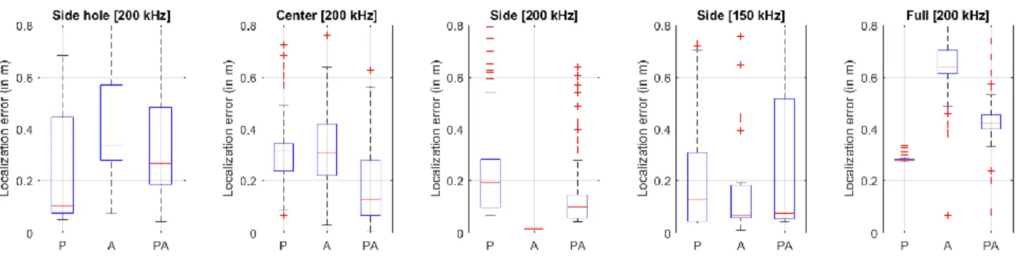
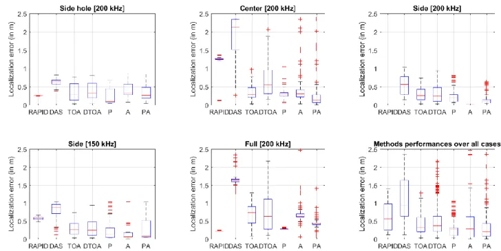
Figure 5: Summary of the localization results for the 100 localization trials, for the different investigated cases, and for the different damage localization indexes. Red lines indicate median values, blue boxes the upper and lower interquartile ranges.
A summary of the localization results for each case under study and for each damage localization index is provided in Figure 5. In this figure, each subplot corresponds to a given case, as described above. For each case, a statistical summary of the 100
localization runs is plotted in terms of localization error, i.e. in terms of distance between the maximum of the damage localization index and the actual damage position. In these plots, the red lines indicate median values, the blue boxes the upper and lower interquartile ranges, the whiskers extend to the most extreme data points the algorithm considers not to be outliers, and the outliers are plotted individually as red “+”.
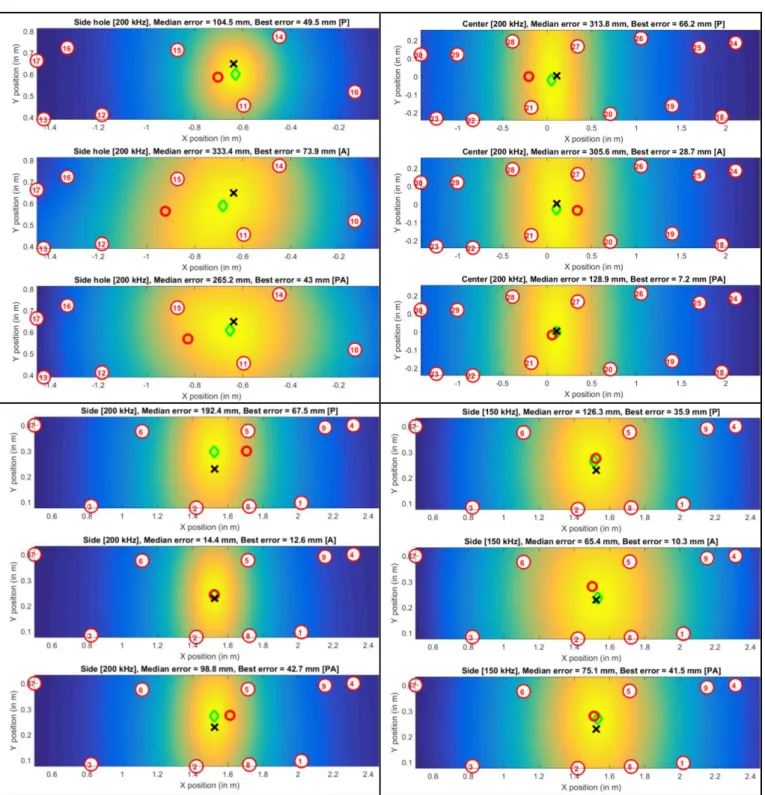
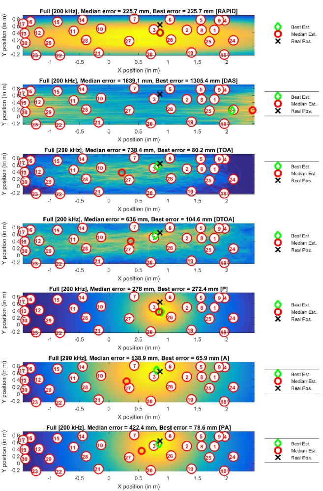
Fig. 6: Overview of the localization results for the different damage localization indexes and for the different substructures under study. For each method, the black “x” stands for the actual damage position, the red circle for the median estimated position and the green diamond for the best estimated position.
From Figure 5, it can be seen that for the cases “Center”, ‘Hole” and “Side”, an average damage localization precision around 10 𝑐𝑚 is obtained by using the proposed algorithm whatever the damage localization index being considered. Furthermore, when considering only “Center” and “Side” substructure, it can be seen that the damage localization indexes that make use of the amplitude information or of both the phase and amplitude information provide results that are slightly better than the damage localization index relying only on the phase information. This is not the case for the structure “Hole” for which results are better when considering the phase information than when adding amplitude information. This may be due to the presence of the hole which potentially has a large effect on amplitude. When looking at the effect of the frequency for the case “Side”, it can be observed that localization results obtained at 150 𝑘𝐻𝑧 are on average as precise as the ones obtained at 200 𝑘𝐻𝑧 but that there is more dispersion of the results with the lower frequencies. This can be linked to the fact that when the frequency increases, the wavelength diminishes. When considering the results obtained for the “Full” case, it can be seen that the average localization error is around 30 cm and that as observed in the “Hole” case, the addition of the amplitude information leads to less precise results. Again, this could be attributed to the complex geometry of the fan cowl, being equipped with many stiffeners. In summary, with this algorithm an average localization precision of 10 cm is achievable (see Figure 5) and that the addition of the amplitude information can be beneficial for cases where the geometry remains rather simple.
More detailed localization results are provided in Fig. 6 and Fig. 7. On these figures, the damage localization indexes P(𝑀), A(𝑀) or PA(𝑀) are plotted for each case under study. In addition to the resulting damage localization maps, the position of the actual damage as well as the position of the best estimation and of the median estimation provided by the algorithm are provided. Furthermore, the associated “Best errors” and “Median errors’ are reported in the title of each subplot. From these figures, it can be seen that the median estimated localization for each case under study lies relatively close to the actual damage position, which is in good agreement with results presented in Figure 5. It can also be seen that the damage localization maps provided by the various damage localization indexes graphically indicate the correct area and that for each case being studied the best localization results are really close to the actual damage position. This error can be as low as 7 mm as observed here for the “Center” case which is rather encouraging. When focusing on Fig. 7, it can be seen that the localization error is larger than for the other cases. This has to be balanced with the fact that the structure being studied is itself larger. Thus, the relative localization error (i.e. the localization error divided by the larger portion of the structure expressed in %) is ≃ 4 − 7% for all the cases being considered.
3.4 Comparison with standard methods from the literature
Figure 8: Comparison of the performances of the tensor-based localization algorithm with standard localization methods from the literature over the 100 localization trials and for the different investigated cases. RAPID: Reconstruction algorithm for probabilistic inspection of defects [48]. DAS: Delay-and-sum method [38]. TOA: Time of arrival or ellipse method [24]. DTOA: Difference time of arrival or hyperbola method [24]. Red lines indicate median values, blue boxes the upper and lower interquartile ranges.
To highlight the originality of the proposed tensor-based damage localization approach and to compare it with other approaches, it is now compared to other standard approaches from the literature. In the literature review presented in Section 1, several classes of damage localization methods emerged. Some classes used no a priori information regarding the structure (“time”,
“amplitude”, and “delay and sum classes” of methods) whereas the others rely on a physical model of wave propagation and thus on the knowledge of some structure material properties (“correlation” and “sparse” classes of methods). In order to compare only blind methods – i.e. methods that do not require prior information with respect to the mechanical properties of the structures under study - the retained approaches for performance comparison are the reconstruction algorithm for probabilistic inspection of defects (RAPID, see [48] for implementation details), the standard delay-and-sum method (DAS, see [38] for implementation details), the time of arrival or ellipse method (TOA, see [24] for implementation details) and the difference time of arrival or hyperbola method (DTOA, see [24] for implementation details). As in Figure 5, a summary of the localization results for each case under study and for each damage localization method mentioned above is provided in Figure 8. In this figure, each subplot corresponds to a given case, as described above, and the last subplot gathers localization errors for all the studied cases. For each case, a statistical summary of the 100 localization runs is plotted in terms of localization error, i.e. in terms of distance between the maximum of the damage localization index and the actual damage position. In these plots, the red lines indicate median values, the blue boxes the upper and lower interquartile ranges, the whiskers extend to the most extreme data points the algorithm considers not to be outliers, and the outliers are plotted individually as red “+”. From this figure it can be seen first that the delay-and-sum method provides localization errors that are significantly larger than the errors reported for the other methods. Thus, even if providing accurate results for academic cases [27, 28, 29, 30, 31, 32], this method do not seem to be robust to a geometrically complex structure, at least in its simpler implementation. When looking at the performances of the ellipse and hyperbola methods, whatever the considered use-case, their median error remains acceptable. However, by looking at the dispersion around this median error, localization results are widespread over a wide range of values which warrants the use of such methods for these complex structures even if again such methods provide satisfactory results in academic cases [18, 19, 20, 21, 22, 23, 24]. Finally, the analysis of the results provided by the reconstruction algorithm for probabilistic inspection of defects (RAPID, see [48]) show a very small dispersion of the results but with sometimes a median localization error that can reach rather high levels. In conclusion, in comparison with the selected localization methods the tensor-based localization algorithm provides results that are at the same time more precise (the median error is the lower one) and less variable (the interquartile range is the smaller) of all the tested methods at least for the cases under study. More detailed localization results are provided in Fig. 7. On this figure, the damage localization maps are plotted for each case under study and for each reference method at hand (DAS, ellipse- and hyperbola-based). In addition to the resulting damage localization maps, the position of the actual damage as well as the position of the best estimation and of the median estimation provided by the different algorithms are provided. Furthermore, the associated “Best errors” and “Median errors’ are again reported in the title of each subplot. This figure confirms the global tendency observed in Figure 8. It is thus demonstrated for the present geometrically complex case study that the proposed tensor-based approaches (P, A and PA) are on average the most precise and robust one: over all the tested cases, they exhibit the lowest median error and smaller localization error while keeping standard deviations comparable or smaller than other methods.
4. DISCUSSION
4.1 Ability to handle complex geometrical structures
Performances of the tensor-based damage localization algorithm have been highlighted in the previous section over various cases. Considered cases where geometrically complex and challenging for the proposed damage localization algorithm. For example, the “Hole” case where a hole exists in the structure or the “Full” case for which the structure is equipped with several stiffeners. Clearly, the results show that the tensor-based damage localization is able to handle such geometrically complex structures and to provide localization results with an acceptable precision for structural health monitoring. One explanation regarding the ability of the algorithm to handle complex geometry is that it relies on two sources of information, namely phase and amplitude, that are sensitive to geometrical complexities in different manners. Furthermore, with the proposed approach, the information coming from all path are merged together during the optimization process that leads to the canonical polyadic decomposition. This optimization process is trying to find the “most suitable” damage localization given the information sources at hand. Such an optimization algorithm thus naturally discards information sources that are not coherent with most of the information sources. Such incoherent information can come from the geometrical complexity of the structure (stiffener or holes here for example). Thus, the combination of these two sources of information (phase and amplitude) in addition to the canonical polyadic decomposition (which is an optimization algorithm) appears to be efficient for the proposed approach to manage geometrically complex structures. In order to support that claim, the algorithm is directly validated on an industrially relevant case with many piezoelectric elements and many structural complexities.
4.2 Qualitative comparison with standard damage localization approaches
The increased performances in terms of precision and robustness of the proposed method do not come from a better understanding of the physical wave propagation phenomenon as the model retained here remains relatively simple. The fact that the tensor-based damage localization algorithm performs better than the standard method comes from the fact that this algorithm does not rely on any empirical or arbitrary data fusion algorithm. Indeed, for all the concurrent methods, the analysis is performed locally (i.e. path-by-path). This means that for all these methods, one damage localization map is built up for each path and
afterwards all these damage localization maps are summed arbitrarily altogether (see for example Eq. 12 in [49], Eq. 22 in [27], Eq. 31 in [33] or Eq. 4 in [48]). Such a strategy absolutely does not consider the fact that information extracted from one path may be in adequation with the information extracted from the other paths or totally incoherent with it. Consequently, using such approaches coherent and incoherent information sources are mixed together with the incoherent sources polluting the coherent ones. For example, when looking at Fig.3, the longest interval of PZT pair considered here (e.g. between the elements 23 and 24) is about 4m while the amplitude of the excitation signal is only 10V. Intuitively, it is expected that the sensor signal would be too weak to use and this is actually the case. This path thus constitutes a typical incoherent source of information as it contains only noise. However, this path will be processed by standard algorithms as any other path and will thus contribute in blurring the overall damage localization map. The advantage of the proposed approach is thus that information coming from all paths are merged together during the optimization process that leads to the canonical polyadic decomposition. This optimization process is trying to find the “most suitable” damage localization given the information sources at hand. Such an optimization algorithm thus naturally discards information sources that are not coherent with most of the information sources and thus naturally provides better results. This is the main qualitative features that differentiate the proposed approach from standard damage localization approach and that makes it more precise and robust on the proposed real scale examples.
4.3 Underlying physical assumptions
The assumptions made when describing the underlying intuitive physical wave propagation model can also be discussed. It is assumed here that only the 𝑆0 mode propagates, that the propagation is isotropic, and that the attenuation is exponential. The
underlying idea here is not that the above-mentioned assumptions describe exactly the structure under study. What is just needed is a reasonable (but approximated) semi-blind framework from which relevant information regarding damage location can be extracted. And even with these approximated assumptions, the results can be found as acceptable.
Indeed, Lamb wave propagation in composite materials is multimodal and involves both the 𝑆0 and the 𝐴0 modes in the
lower frequency range. However, the 𝐴0 mode propagates much slower than the 𝑆0 mode in composite materials at the frequencies of interest. Furthermore the 𝑆0 mode is not dispersive in the selected frequency range whereas 𝐴0 is. Consequently,
as the present method only focuses on the first and thus fastest wave packet, only the 𝑆0 mode is considered and the 𝐴0 is
discarded in cases when it is excited by a piezoelectric element or when it results from a mode conversion phenomenon. This justifies why only the first wave packet of the 𝑆0 mode is modelled here. However, it is still possible to set up a more realistic
physical model on which tensor representation and decomposition can be investigated. For example, if it is possible to separate the contributions of both the 𝐴0 and 𝑆0 modes within the received signals (for example by means of dual piezoelectric elements
[47]), then more information would be available and packed within the tensor representation. Indeed, it is possible to use the same model for the 𝐴0 mode than for the 𝑆0 mode (obviously with different wave velocity and attenuation coefficients) and to
build for 𝐴0 a tensor representation from which damage localization information can be extracted and added to the information
extracted from 𝑆0.
It would also have been possible to compute the dispersion curves for Lamb wave propagating in the structures under study. One drawback of such an approach is that material properties associated with the structure under study are then needed. Here, the objective is to provide a method that needs no parameter tuning. This explains why it has been chosen not to rely on dispersion curves. Furthermore, the only information that could have been brought by dispersion curves would have been the approximate knowledge of Lamb wave propagation velocities, which can also be estimated from data available in the healthy state.
Furthermore, wave propagation in each composite material ply is known to be highly anisotropic. However, the plies are generally arranged in such a way that seen from total thickness propagation may be considered as almost isotropic within the framework of the proposed semi-blind approach [24, 47]. Regarding the exponential decay of the amplitude with distance, this assumption is true only in the far field, i.e. when lying enough wavelength away from the emission point which is the piezoelectric element. As here the wavelength for the 𝑆0 mode is around 2 cm and given the structures sizes, this assumption appears as
acceptable.
Additionally, the selected physical model has been restrained here only to the single damage case. However, it can be easily extended to the multi-damage case. Indeed, one additional damage will manifest itself by an additional echo within the recorded difference signals and thus by an additional term in Eq. 3. A theoretical analysis of these additional terms could be performed to assess how it impacts the phase and amplitude tensors and if several damage can be located simultaneously by means of the proposed algorithm.
4.4 Algorithm robustness
The last point to mention in this discussion is related to the fact that the proposed algorithm appears to be relatively robust and that it does not rely on specific pre-processing steps or any external parameters that need to be finely tuned. The only needed input parameters are the number of samples (1500 here for each case) and the frequency bounds over which the frequency analysis has to be performed (between 0.9𝑓0 and 1.1𝑓0 here). The influence of these parameters has not been found to be crucial
and keeping the same parameters values for all the cases as done above leads to acceptable localization results. As a consequence, the proposed algorithm is relatively robust. In terms of localisation performances, the best localization error, is around 7 𝑚𝑚 for a structure that is 4 𝑚 long (see the “Center” case), which from our point of view is a promising result In practice, the actual damage position is not known, and it is not possible to define a “best localization”., However, it's possible to rely on the mean
or median estimated localization. And as demonstrated by the above results, the median estimated localization over 100 localization runs is relatively close to the actual damage position and is thus a reliable information regarding damage location for SHM with a relative error ≃ 4 − 7% of the structure under study.
Another point to mention here is that there exist absolutely no constraints on piezoelectric localization to run this algorithm. The piezoelectric elements have been regularly placed along the structure, by ensuring that they were not too close to the stiffeners or to the structures border while being not too far away from each other to guarantee that enough signal is received. In conclusion, the algorithm does not rely on any special sensor configuration and can thus adapt to any sensor network configuration as long as it is physically reasonable.
5. CONCLUSION
Monitoring in real time and autonomously the health state of aeronautic structures is referred to as Structural Health Monitoring (SHM) and is a process decomposed in four steps: damage detection, localization, classification, and quantification. Structures under study are here geometrically complex aeronautics structures and the focus is put on the localization step of the SHM process. The fact that SHM data are naturally three-way tensors is here investigated for this purpose. It is demonstrated that under classical assumptions regarding wave propagation, the canonical polyadic decomposition of rank 2 of the tensors built from the phase and amplitude of the difference signals between a healthy and damaged states provide direct access to the distances between the piezoelectric elements and damage. This property is used here to propose an original tensor-based damage localization algorithm. This algorithm is successfully validated on experimental data coming from a scale one part of an airplane nacelle (1.5 m in height for a semi circumference of 4 m) equipped with 30 piezoelectric elements and many stiffeners. Obtained results demonstrate that the tensor-based localization algorithm is able to locate a damage within this structure with an average precision of 10 cm and with precision lower than 1 cm at best. Furthermore, it is important to notice that this algorithm onl y takes the raw signals as inputs and that no specific pre-processing step or external parameters need to be finely tuned.
Finally, it is important to remind the whole pre-processing process which is at the basis of the proposed algorithm. First the time signals are filtered around the central excitation frequency and then the first wave packet is isolated. Due to measurement noise, some of these steps may fail or provide unappropriated results. So, the first challenge faced here was to have an algorithm robust to noise. Then, the localization process relies on a simplified model of wave propagation within the structure (one mode propagating, no dispersion, isotropy) that may not fit the reality especially for complex geometrical structures. Thus, the second challenge to overcome was to build an algorithm robust to model errors. In summary, as compared to a standard A4 plates nicely hanged out in a laboratory, the challenges faced here were to build up algorithms robust to noise and to model errors. In this sense, the proposed method thus appears as a step forward closing the gap between research and industrial deployment for structural health monitoring [9].
REFERENCES
[1] D. Balageas, C.-P. Fritzen et A. Güemes, Structural health monitoring, vol. 493, Wiley Online Library, 2006. [2] C. R. Farrar et K. Worden, «An introduction to structural health monitoring,» Philosophical Transactions of the
Royal Society of London A: Mathematical, Physical and Engineering Sciences, vol. 365, pp. 303-315, 2007. [3] K. Worden, C. R. Farrar, G. Manson et G. Park, «The fundamental axioms of structural health monitoring,»
Proceedings of the Royal Society of London A: Mathematical, Physical and Engineering Sciences, vol. 463, pp. 1639-1664, 2007.
[4] C. R. Farrar et K. Worden, Structural health monitoring: a machine learning perspective, John Wiley & Sons, 2012.
[5] M. Mitra et S. Gopalakrishnan, «Guided wave based structural health monitoring: A review,» Smart Materials and Structures, vol. 25, p. 053001, 2016.
[6] A. Raghavan et C. E. S. Cesnik, «Review of guided-wave structural health monitoring,» Shock and Vibration Digest, vol. 39, pp. 91-116, 2007.
[7] Z. Su et L. Ye, Identification of damage using Lamb waves: from fundamentals to applications, vol. 48, Springer Science & Business Media, 2009.
[8] S. Zhongqing, Y. Lin et L. Ye, «Guided Lamb waves for identification of damage in composite structures: A review,» Journal of Sound and Vibration, vol. 295, p. 753–780, 2006.
[9] P. Cawley, «Structural health monitoring: Closing the gap between research and industrial deployment,» Structural Health Monitoring, p. 1475921717750047, 2018.
[11] N. D. Sidiropoulos, L. De Lathauwer, X. Fu, K. Huang, E. E. Papalexakis et C. Faloutsos, «Tensor decomposition for signal processing and machine learning,» IEEE Transactions on Signal Processing, vol. 65, pp. 3551-3582, 2017. [12] H. Fanaee-T et J. Gama, «Tensor-based anomaly detection: An interdisciplinary survey,» Knowledge-Based
Systems, vol. 98, pp. 130-147, 2016.
[13] P. Cheema, N. L. D. Khoa, M. Makki Alamdari, W. Liu, Y. Wang, F. Chen et P. Runcie, «On Structural Health Monitoring Using Tensor Analysis and Support Vector Machine with Artificial Negative Data,» chez Proceedings of the 25th ACM International on Conference on Information and Knowledge Management, 2016.
[14] M. A. Prada, J. Toivola, J. Kullaa et J. HollméN, «Three-way analysis of structural health monitoring data,» Neurocomputing, vol. 80, pp. 119-128, 2012.
[15] R. You, Y. Yao et J. Shi, «Tensor-based ultrasonic data analysis for defect detection in fiber reinforced polymer (FRP) composites,» Chemometrics and Intelligent Laboratory Systems, vol. 163, pp. 24-30, 2017.
[16] R. Zheng, K. Nakano, R. Ohashi, Y. Okabe, M. Shimazaki, H. Nakamura et Q. Wu, «PARAFAC Decomposition for Ultrasonic Wave Sensing of Fiber Bragg Grating Sensors: Procedure and Evaluation,» Sensors, vol. 15, pp. 16388-16411, 2015.
[17] Z. Su, L. Ye et Y. Lu, «Guided Lamb waves for identification of damage in composite structures: A review,» Journal of sound and vibration, vol. 295, pp. 753-780, 2006.
[18] M. Lemistre et D. Balageas, «Structural health monitoring system based on diffracted Lamb wave analysis by multiresolution processing,» Smart materials and structures, vol. 10, p. 504, 2001.
[19] P. S. Tua, S. T. Quek et Q. Wang, «Detection of cracks in plates using piezo-actuated Lamb waves,» Smart Materials and Structures, vol. 13, p. 643, 2004.
[20] J. Moll, R. T. Schulte, B. Hartmann, C. P. Fritzen et O. Nelles, «Multi-site damage localization in anisotropic plate-like structures using an active guided wave structural health monitoring system,» Smart Materials and Structures, vol. 19, p. 045022, 2010.
[21] C. Zhou, Z. Su et L. Cheng, «Probability-based diagnostic imaging using hybrid features extracted from ultrasonic Lamb wave signals,» Smart Materials and Structures, vol. 20, p. 125005, 2011.
[22] B. Li, Y. Liu, K. Gong et Z. Li, «Damage localization in composite laminates based on a quantitative expression of anisotropic wavefront,» Smart Materials and Structures, vol. 22, p. 065005, 2013.
[23] G. Yan, «A Bayesian approach for damage localization in plate-like structures using Lamb waves,» Smart Materials and Structures, vol. 22, p. 035012, 2013.
[24] C. Fendzi, N. Mechbal, M. Rebillat, M. Guskov et G. Coffignal, «A general Bayesian framework for ellipse-based and hyperbola-ellipse-based damage localization in anisotropic composite plates,» Journal of Intelligent Material Systems and Structures, vol. 27, pp. 350-374, 2016.
[25] L. Wang et F. G. Yuan, «Active damage localization technique based on energy propagation of Lamb waves,» Smart Structures and Systems, vol. 3, pp. 201-217, 2007.
[26] J. E. Michaels et T. E. Michaels, «Damage localization in inhomogeneous plates using a sparse array of ultrasonic transducers,» chez AIP Conference Proceedings, 2007.
[27] C. H. Wang, J. T. Rose et F.-K. Chang, «A synthetic time-reversal imaging method for structural health monitoring,» Smart materials and structures, vol. 13, p. 415, 2004.
[28] J. E. Michaels et T. E. Michaels, «Guided wave signal processing and image fusion for in situ damage localization in plates,» Wave motion, vol. 44, pp. 482-492, 2007.
[29] C.-T. Ng et M. Veidt, «A Lamb-wave-based technique for damage detection in composite laminates,» Smart materials and structures, vol. 18, p. 074006, 2009.
[30] J. S. Hall, P. McKeon, L. Satyanarayan, J. E. Michaels, N. F. Declercq et Y. H. Berthelot, «Minimum variance guided wave imaging in a quasi-isotropic composite plate,» Smart Materials and Structures, vol. 20, p. 025013, 2011. [31] Z. Sharif-Khodaei et M. H. Aliabadi, «Assessment of delay-and-sum algorithms for damage detection in
aluminium and composite plates,» Smart materials and structures, vol. 23, p. 075007, 2014.
[32] C. Haynes et M. Todd, «Enhanced damage localization for complex structures through statistical modeling and sensor fusion,» Mechanical Systems and Signal Processing, vol. 54, pp. 195-209, 2015.
[33] L. Yu et V. Giurgiutiu, «In situ 2-D piezoelectric wafer active sensors arrays for guided wave damage detection,» Ultrasonics, vol. 48, pp. 117-134, 2008.
[34] N. Quaegebeur, P. Masson, D. Langlois-Demers et P. Micheau, «Dispersion-based imaging for structural health monitoring using sparse and compact arrays,» Smart Materials and Structures, vol. 20, p. 025005, 2011.
[35] N. Quaegebeur, P. C. Ostiguy et P. Masson, «Correlation-based imaging technique for fatigue monitoring of riveted lap-joint structure,» Smart Materials and Structures, vol. 23, p. 055007, 2014.
[36] P.-C. Ostiguy, A. Le Duff, N. Quaegebeur, L.-P. Brault et P. Masson, «In situ characterization technique to increase robustness of imaging approaches in structural health monitoring using guided waves,» Structural Health Monitoring, vol. 13, pp. 525-536, 2014.
[37] A. Ebrahimkhanlou, B. Dubuc et S. Salamone, «Damage localization in metallic plate structures using edge-reflected lamb waves,» Smart Materials and Structures, vol. 25, p. 085035, 2016.
[38] P.-C. Ostiguy, N. Quaegebeur et P. Masson, «Comparison of model-based damage imaging techniques for transversely isotropic composites,» Structural Health Monitoring, vol. 16, pp. 428-443, 2017.
[39] R. Levine et J. E. Michaels, «Block-sparse reconstruction and imaging for lamb wave structural health monitoring,» IEEE transactions on ultrasonics, ferroelectrics, and frequency control, vol. 61, pp. 1006-1015, 2014. [40] A. Golato, F. Ahmad, S. Santhanam et M. G. Amin, «Multipath exploitation for enhanced defect imaging using
Lamb waves,» NDT \& E International, vol. 92, pp. 1-9, 2017.
[41] M. Gresil et V. Giurgiutiu, «Prediction of attenuated guided waves propagation in carbon fiber composites using Rayleigh damping model,» Journal of Intelligent Material Systems and Structures, vol. 26, pp. 2151-2169, 2015. [42] H. Mei et V. Giurgiutiu, «Guided wave excitation and propagation in damped composite plates,» Structural
Health Monitoring, vol. 0, p. 1475921718765955, 0.
[43] P. K. P. M. W. O. Tomasz Wandowski, Guided wave attenuation in composite materials, vol. 10170, 2017, pp. 10170 - 10170 - 9.
[44] K. Ono et A. Gallego, «Attenuation of Lamb Waves in CFRP Plates.,» Journal of Acoustic Emission, vol. 30, 2012.
[45] N. Vervliet, O. Debals, L. Sorber, M. Van Barel et L. De Lathauwer, «Tensorlab 3.0,» 2016.
[46] C. Fendzi, M. Rebillat, N. Mechbal, M. Guskov et G. Coffignal, «A data-driven temperature compensation approach for Structural Health Monitoring using Lamb waves,» Structural Health Monitoring, vol. 15, pp. 525-540, 2016.
[47] E. Lize, M. Rebillat, N. Mechbal et C. Bolzmacher, «Optimal dual-PZT sizing and network design for baseline-free SHM of complex anisotropic composite structures,» Smart Materials and Structures, 2018.