Error Estimation for Model Order Reduction of Finite Element Parametric Problems

(1)

is an open access repository that collects the work of Arts et Métiers Institute of

Technology researchers and makes it freely available over the web where possible.

This is an author-deposited version published in: https://sam.ensam.eu

Handle ID: .http://hdl.handle.net/10985/11034

To cite this version :

Stéphane CLENET, Thomas HENNERON - Error Estimation for Model Order Reduction of Finite Element Parametric Problems - IEEE Transaction on Magnetics - Vol. 52, p.1-10 - 2016

Any correspondence concerning this service should be sent to the repository Administrator : archiveouverte@ensam.eu

(2)

Error Estimation for Model Order Reduction of Finite Element

Parametric Problems

S. Clénet

1

and T. Henneron

2

1_{L2EP, Arts et Métiers ParisTech, 59046 Lille, France.} 2_{L2EP, Université Lille 1, 59655 Villeneuve d’Ascq, France.}

To solve a parametric model in computational electromagnetics, the Finite Element method is often used. To reduce the computational time and the memory requirement, the Finite Element method can be combined with Model Order Reduction Technic like the Proper Orthogonal Decomposition (POD) and the (Discrete) Empirical Interpolation ((D)EI) Methods. These three numerical methods introduce errors of discretisation, reduction and interpolation respectively. The solution of the parametric model will be efficient if the three errors are of the same order and so they need to be evaluated and compared. In this paper, we propose an a-posteriori error estimator based on the verification of the constitutive law which estimates the three different errors. An example of application in magnetostatics with 11 parameters is treated where it is shown how the error estimator can be used to control and to improve the accuracy of the solution of the reduced model.

Index Terms— Finite Element Method, Model Order Reduction, POD method, (D)EI method, error estimation, adaptive procedure

I. INTRODUCTION

inite Element (FE) models are now the standard to study electromagnetic devices like electrical machines, transformers because they are so accurate that they can be considered as a virtual prototype. However, for the design of electromagnetic device, these models cannot be used during the whole process of design but only at the end because of their computational time. In fact, at the beginning of the design process, the space of parameters has to be explored which requires a huge amount of model runs. To circumvent this issue, an analytical model based on physical considerations and much faster than a FE model is associated. The issue is then the relationship between the solutions given by the FE model and the analytical model which does not explicitly exists, that is to say that it is not straightforward to reconstruct a solution obtained by the analytical model in the FE space and reversely to take advantage of the FE solution to improve the accuracy of the analytical model. Model Order Reduction (MOR) methods have been proposed in order to reduce the computational time and the memory storage requirement [1-4]. Among these methods, Proper Orthogonal Decomposition methods (or derived method like the Reduced Basis method) which consist in searching an approximate solution in a subspace of the FE space spanned by FE model solutions, so called snapshots. This method has been applied successfully to solve non-linear problems in time domain in computational electromagnetics [5-8] and also to solve parametric models [9-12]. The POD solution can be easily projected in the space of the FE solution providing a natural link with the full FE model. Moreover, the accuracy of the POD model can be improved by introducing “naturally” any new FE model solution (snapshot). The key point is then the control of the accuracy of the POD model which depends highly on the choice of the snapshots. A posteriori error estimators have been proposed in the literature to evaluate the error introduced by the process of reduction. This error estimator is then applied along with a greedy algorithm or

other self-adaptive procedures [12-16].

If the equation system, derived from the parametric FE model, is affine in parameters that is to say it is written under the form of a sum of terms equal to the product of a constant matrix and a function of the parameters of the problem, the Reduced Basis can be derived which can really alleviate the memory requirement and the computational time. Deriving an affine expression from the FE model is not always possible, approximation methods like (Discrete) Empirical Interpolation ((D)EI) method can be applied in order to obtain an approximation under an affine form [17,18]. An error, so-called interpolation error in the following, arises which needs also to be evaluated.

Moreover, when applying a model order reduction technic in the literature, the FE model is often assumed to be perfect in the sense the discretization error due to the application of the FE method is negligible. It is assumed that the FE solution is equal to the exact solution of the partial differential equation system. In practice, this is not true and the discretization error always exists and should be also controlled.

To summarize, we have finally three errors, which are the discretization error intrinsic to the FE method, the reduction error introduced by the MOR method and finally the interpolation error due to the approximation by an affine system of equations of the original FE model. These errors have to be compared to each other. For example, if the error of discretization is about 10 percent it is useless to obtain a error of reduction of less than one percent because it won’t improve much the accuracy of the POD model providing that the increasing of POD model accuracy comes along with an increasing of its construction and computational time.

At least in computational electromagnetism, the simultaneous estimation of the three errors has not been treated in the literature. For example in [12], a method is proposed to construct adaptively a reduced model from a finite element model, without applying the offline/online method. The adaptive construction is based on an error estimator which enables to evaluate only the reduction error without

F

(3)

considering the error of discretisation due to the FE method. Since the (D)EI method was not used in [12] to speed up the solution of the problem, no approximation error was also considered.

In this paper, we propose a unique error estimator which can be applied to evaluate the three kinds of errors and which enables to control the accuracy of the full process of reduction. This error estimator is based on the verification of the constitutive relationship which has been already successfully used to estimate the discretization error [19,20]. This error estimator can be incorporated in an adaptive procedure in order to determine automatically the snapshots and the affine interpolation.

The paper is organized as follow. In order to introduce the notation, the two FE potential formations in magnetostatic are presented. The principle of the error estimator based on the verification of the constitutive relationship is recalled. Then, the parametric FE model is detailed particularly the technic to account for geometric parameters. The reduction methods like POD method and (D)EI method are presented as well as their combination. The error estimator enabling to evaluate the three sources of errors is then introduced. Finally, the proposed approach is applied to reduce a FE model of a magnetic holder with 11 parameters. It is shown how the proposed error estimator enables to evaluate the different kinds of error and how it can be applied to obtain an accurate reduced model.

II. MAGNETOSTATIC FEMODEL

A. Magnetostatic problem

We will consider an electromagnetic device which can be described by the magnetostatic equations on a domain D. In this section, we aim at introducing the notations. All the dimensions, the constitutive law of the materials and the sources are supposed to be set. The equations to be solved are:

curl H(x) = J(x) (1)

div B(x) = 0 (2)

with H(x) the magnetic field, B(x) the magnetic flux density and J(x) the current density, which its distribution is assumed to be known. In addition, conditions on H(x) and B(x) are added on the boundary G of the domain D:

n(x)×H(x)=0 on GH (3) n(x)⋅B(x)=0 on GB (4)

With GH∩GB=0, GH∪GB=G and n(x) the outward normal

vector. Finally, the fields H(x) and B(x) satisfy the constitutive law:

Η(x)=ν(x) [B(x)-Br(x)] (5)

With ν(x) the magnetic reluctivity and Br(x) the remanent

magnetic flux density. In practice, the domain D is often divided into K subdomains Dk on which the reluctivity (resp.

the remanent flux density) is constant and equal to νk (resp Brk). The reluctivity ν(x) and the remanent magnetic flux Br(x)

can be written under the form:

( )

∑

( )

∑

= =ν = = ν K 1 k k K 1 k k kI (x) B x B I (x) x r rk (6)

With Ik(x) a function equal to 1 if x belongs to Dk and 0

elsewhere. To solve a system of Partial Differential Equations (PDE) given by (1), (2) and (5), two FE potential formulations can be used.

B. Vector potential formulation

In the case of the vector potential formulation, the magnetic flux density is expressed under the form: curlA(x) = B(x) and

A(x)×n(x)=0 on GB. Combining (1) and (5), the PDE to solve

reads:

curl [ν(x) curlA(x)] = J(x)+ curl [ν(x) Br(x)] (7)

To find an approximation of the solution, the FE method is generally applied. An approximation of the vector potential

AEF(x) is sought in the edge element space such that [21]:

( )

∑

= = N 1 j j j ( ) a w x x A_EF (8)

with N the number of Degrees of Freedom (DoF’s), wi(x) the

edge shape functions and ai unknown real coefficients. By

applying the Galerkin method to a weak form of (7), N equations are obtained:

( )

[

( ) ( )

]

( )d i

[ ]

1,N )d ( ) ( ) ν( i r D i ∈ ∀ ⋅ + = ⋅

∫

D x x w x B x curl x J x x curlw x curlA x EF ν (9)

Replacing AEF(x) by its expression (8) in (9), we obtain N

linear equations which can be written under the form:

SA XA = FA (10)

with SA the stiffness matrix (N×N), FA the source vector (N×1) and XA the vector of the coefficients ai. The coefficients

sij of S and fi of F satisfy:

( )

[

]

∫

⋅ + = ⋅ = D i r i D j i ij )d ( ) ( ) ( f )d ( ) ( ) ν( s x x curlw x B x curl x J x x curlw x curlw x ν (11)

C. Scalar potential formulation

According to (1), the magnetic field H can be expressed as a function of the gradient of a scalar potential Ω: H=Hs-gradΩ

with Ω(x)=Cste on GH. The source field Hs is defined such that

curlHs(x)=J(x) with Hs(x)×n(x)=0 on GH. Combining (2) and

(5), the PDE in the case of the scalar potential formulation is: div [ν(x)-1grad Ω(x)] =div[ν(x)-1Hs(x)]-div[Br(x)] (12)

Similarly to the vector potential formulation presented before (see (8)), an approximation ΩEF is expressed in the finite

dimensional space (the nodal element space). Applying the Galerkin method to a weak form of (12) leads to solve a system of linear equations under the form (10), SΩ XΩ = FΩ

(4)

III. ERROR ESTIMATION

The application of the FE method leads to an error of discretization. If (Bex(x),Hex(x)) denotes the exact solution of

the problem (the solution satisfies (1)-(5)) in the continuous domain, the solution BEF(x)=curlAEF(x) of the FE vector

potential formulation (7) is not equal to Bex(x) in the general

case. This is the same for the solution HEF(x) of the scalar

potential formulation. The couple (BEF(x),HEF(x)) satisfies the

equations (1)-(4) but not the behavior law (5). The term e2=||HEF(x)-ν(x)[BEF(x)-Br(x)]||2ν (13) with: _ν =

∫

ν− ⋅ D )d ( ) ( ) ( ) (x xV x Vx x V 2 1

is always positive and is equal to zero when the equation (5) is satisfied that is to say that the couple(BEF(x),HEF(x)) is

equal to the exact solution. Moreover, it can be shown that: e2=||HEF(x)-Hex(x)||2ν +||BEF(x)-Bex(x)||21/ν

The diminution of the value of e2 means that the solution is closer to the exact solution. The term e2 gives an estimation of the error of discretization introduced by the FE method. Finally, solving the two potential formulations on the same mesh M leads to a couple (BEF(x),HEF(x)) which enables to

estimate the error due to the FE method by calculating (13). We can also define a relative error ε:

2 1 2 ν ν+ = ε / ) ( ) ( 4e2 x B x H_EF _EF (14)

This error estimator based on the verification of the constitutive relationship has been widely used to control the quality of the FE mesh. The aim of this paper is to extend the domain of application of this estimator to the reduction of parametric model. To introduce that, we will present in the following the parametric model and the model order reduction technics in the case of the vector potential formulation but the extension to the scalar potential formulation is straightforward.

IV. PARAMETRIC FEMODELS

A. Parametric Finite Element Model

Let consider now that some inputs of the model like dimensions, reluctivities νk of some materials or currents in

some stranded inductors are not fixed. This situation can arise during a design process where the inputs are the unknowns of the problem and should be fixed in order to satisfy given criteria of performances. The inputs can also be considered as unknown because of a lack of knowledge or because they are intrinsically variables and subject to dispersion. These inputs are then considered as parameters. We denote p=(p1,..,pP) the

parameter set of dimension P. If the parameterization holds on the magnitude of the source terms (J and Br) or on the material

characteristics νk (see (6)), the same mesh (related only to the

geometry) can be used for any parameter values. The values of

the coefficients sij and fi (see (11)) have to be calculated for

each new set of parameters p and the coefficients ai of XA as

well, which satisfy the system of linear equations dependent on p:

SA(p) XA(p) = FA (p) (15)

The vector potential is then a function of p and we have:

( )

∑

( )

= = N 1 j j j ( ) a ,p pw x x A_EF (16)

The processing of parameterized geometries is slightly different than the processing of the previous kinds of parameterization on the source or the behavior law and it requires additional treatments. An easy way consists in remeshing each geometry corresponding to a new parameter set p. However, this approach has some drawbacks. With a new remeshing for each new parameter set p, the stiffness matrix and the source vector must be recalculated, which is time consuming. Moreover, remeshing the domain D adds a numerical noise on the output data because the mesh (the connectivities between elements, the number of elements…) changes from a parameter set to another. Finally, the expression of the shape functions wi(x) (see (8)) changes as

well. Consequently, it is not obvious to obtain an explicit expression of the vector potential as (16) so the distribution of the fields H(x) and B(x). To avoid the former drawback, one possibility is to introduce additional functions (enrichment basis method) that can account for these discontinuities. This technique has been proposed for the stochastic finite element method in [22,23]. Another possibility consists in applying the transformation method proposed in [24,25] which will be used in the following. It can be shown that the parametrization on the geometry can be transferred on a parametrization on the material characteristics [26]. The unknowns ai of the problem

remain the same whatever the values of the parameter set p and also the connectivities between nodes and elements meaning that the matrix filling of S does not depend on p but only the coefficient values sij and fi. Finally, whatever the kind

of parametrization, the parametric model is given by the system of equations (15). For the design of electromagnetic devices or uncertainty quantification, this system of equations should be solved a numerous number of times which can be very time consuming even unfeasible if the number of unknowns is very high. In the following, we will present MOR method in order to alleviate the calculation time and the memory storage.

V. MODEL ORDER REDUCTION TECHNICS

A. Principles

In the following, we consider P parameters pk each belonging

to an interval [pkmin,pkmax]. The parameter set p=(p1,..,pP)

belongs to the domain

∏

[

]

= = ∆ P 1 k max k min k ,p p .

A Nx×1 vector X(p) of functions defined on ∆ is given. X(p)

can be, for example, the solution XA(p) of the parametric model (15). The vector X(p) can represent also the vector F(p)

(5)

or a vectorised form of the N×N matrix S(p). In the last case, the mth entry xm(p) of X(p) is given by:

xm(p)=sij(p) with m=(j-1)N+i (17)

The idea of MOR technics is to find an approximation of

X(p) under the form:

( )

∑

= ≈ R 1 q q q( ) x p X p X (18)

With Xq Nx×1 vectors with constant entries and xq(p)

functions of p. The reduction holds here in the fact the vector

X(p) does not require the calculation of Nx functions of p but

only R which is supposed to be much lower than N.

Two methods based on the previous principles will be presented in the following: the POD method and the (D)EI method which can be combined efficiently to reduce a FE model.

B. Proper Orthogonal Decomposition (POD) method The POD method, detailed in the following, is one of the most popular MOR methods. Consider Z parameter sets (p1,…,pZ) and the N×Z matrix A of the associated solutions

(XA(p1),…, XA (pZ)) of (15). This matrix A is often so-called

the matrix of snapshots and XA(pi) a snapshot. We define the

linear space K spanned by the vectors (XA(p1),…, XA(pZ)) and

the N×R matrix Ψ (R≤Z) of the vectors (Ψ1,..,ΨR), an

orthogonal basis of the space K. The matrix Ψ can be obtained by a Singular Value Decomposition (SVD) from the matrix A. In fact, the matrix is constructed easily from the EigenValue Decomposition (EVD) of the Z×Z matrix AtA

which is almost costless because Z is equal to several dozen in practice. The idea of the POD method is to seek for an approximation of the solution of (15) in the space K, which means that XA (p) is approximated by the following linear

combination:

( )

∑

( )

= = ≈ R 1 i ri a pΨi p X p XA Ar Ψ (19) The approximation has to satisfy the equation (15), which is not generally possible because the system of equations is overdetermined. The idea is then to cancel the residue SA(p)Ψ

XAr(p)-FA(p) in the space K which is equivalent to solve an

system of R linear equations: Ψt _SA_(p)Ψ_XA

r(p) = Ψt FA(p) (20)

The size of the system (20) is then equal to R, which is much lower than N, the size of the full system (15). The solution of the system of equations is much faster reducing significantly the computational time. However, the accuracy of the method is closely related to the choice of the snapshots (XA(p1),…, XA

(pZ)) used to determine the reduced basis. Moreover, we can

see that we have still to calculate the full matrix SA(p) and the vector FA(p) for each new parameter set p. In the following, we will present the (D)EI method to approximate the matrix

SA(p) and the vector FA(p) in order to reduce their construction time.

C. (Discrete)Empirical Interpolation ((D)EI ) method In the following, we will consider the vector F(p) to present the (D)EI method. However, as it was mentioned in section V-A, the (D)EI method can be applied also on the matrix S(p) by vectorising it as presented in (17). The idea is to approximate

F(p) under the form:

( )

∑

( )

= = = ≈ Q 1 i i DEI p p c pUi F p F U

c

(21)

With c(p)=(c1(p),..,cQ(p)) a vector which entries are linear

combinations of Q “well-chosen entries” of the vector F(p). Then, it is possible to calculate only Q entries of F(p), to compute ci(p) and then, by applying (21), to determine an

approximation FDEI(p) of F(p). This method works very well

if the entries of the vector F(p) are strongly correlated meaning that they vary in the same way with the parameter set

p. In order to determine these Q entries, the vector F(p) is

calculated for Z’ parameter sets (p1,…,pZ’). Then, the

approximation FDEI(p) is sought in the space K’ spanned by

(F(p1),…,F(pZ’)) which correspond to a snapshot matrix F.

Let denote U=(U1,…,UQ), an orthogonal basis of K’ which can

be determined by a Gram-Schmidt Process or a SVD of the snapshot matrix F. Then, by applying the algorithm presented

in Fig. 1, the most “significant” Q entries of F(p) are determined [18]. Let denote I={i1,..,iQ} their indices (1≤ij≤N)

and P the N×Q matrix such that the jth column is the ijth

column eij of the N×N identity matrix. All the entries of P are

equal to zero except the Q entries _i_j j

p (1≤j≤Q). The vector c(p) is then given by:

c(p) = (PtU)-1Pt F(p) (22) The Q×Q matrix (PtU)-1 can be precalculated and the Q entries of the vector PtF(p) are equal to the Q entries of F(p)

with indices belonging to the set I={i1,..,iQ}. Then, F(p) is

approximated by applying (21). With the (D)EI method, only Q entries of F(p) are calculated instead of N, which can save calculation time. However, the accuracy of the approximation should be controlled and depends also on the choice of the parameter sets (p1,…,pZ’). Moreover as shown in the next

section, the system of equations becomes affine in parameter which enables to speed up the computational time of the reduced model.

D. Combination of (D)EI method and POD method Using the (D)EI method and according to (21), an approximation SDEI(p) of the stiffness matrix S(p) can be

written:

( )

∑

( )

= =QS 1 i i DEI p s pVi S (23)

With Vi, Qs sparse matrices with the same data structure as S(p) and si(p) linear combinations of Qs entries of S(p). The

vector F(p) can be approximated also under the form (21) with QF vectors Ui and coefficients ci(p).

Introducing the approximation of S(p) in the reduced model (20), we obtain:

Sr(p) Xr(p)= Fr(p) (24)

(6)

( )

∑

( )

∑

( )

∑

= = = = = = = = F F S S Q 1 i i Q 1 i i r Q 1 i i Q 1 i i r c Ψ c s Ψ Ψ s ri i t ri i t U p U p p F V p V p p S ₍₂₅₎

The R×R matrices Vri and R×1 vectors Uri can be

precalculated. Once these terms are pre-calculated, the construction of the reduced model (24) for a given parameter set p requires only:

-the calculation of the QS entries of S(p) and QF entries of F(p),

-the determination of the vector s(p) and c(p) (see (22) with a pre-calculated matrix (PtU)-1)

-the computation of Sr(p) and Fr(p) using (25).

Consequently, the construction of the reduced model is hugely alleviated because only a small number Qs (resp. QF)

of tiny R×R matrices (resp. Rx1 vectors) are involved in the calculation.

GREEDY ALGORITHM input U=[U1,…,UQ]

output I={i1,…, iQ} and P=(ei1,…,eiQ)

Max() operator

If V=(v1,…,vm) then Max(V)=vj with |vj|≥|vi| i∈{1,…,m}

Initialisation U=[U1] i1=Max(U1) I={i1} P=[eϕ1] For j=2 to Q Solve (Pt S) c = Pt Uj residue=Ui-S c ij=Max(residue)

U=[U,Ui] and P=[P,eϕi] and I={I,ij)

End

Fig. 1: Greedy algorithm to determine the matrix P and the index set I [18]

The combination of the (D)EI method and the POD method is very attractive in terms of computational time. However, as mentionned above, these methods leads to an approximation of the solution and the accuracy of the methods are closely related to the snapshots.

In the following, we will derive an error estimator from the one presented in section III in order to control the accuracy of the reduced model and to determine adaptively the matrix of snapshots.

VI. ERROR ESTIMATION

We consider the solutions XAr(p) and XΩr(p) of two reduced

models derived from the two FE formulations but based on the same mesh M. The two reduced models are obtained after applying either the POD method or the (D)EI method or both. We denote ΨA and ΨΩ , the matrices of the two reduced basis

(see section V-B) and XA(p)=ΨAXAr(p) and XΩ(p)=ΨΩXΩr(p)

the projected solutions in the initial mesh M. If the (D)EI

method is applied alone (which has no practical interest), ΨA and ΨΩ are identity matrices. From the vectors XA(p) and

XΩ(p), two potentials AEF(x,p) and ΩEF(x,p) can be

determined respectively (see (16)). According to section III, an error er2(p) can be calculated from the fields BEF(x,p)=curlAEF(x,p) and HEF(x,p)=Hs(x,p)-gradΩEF(x,p)

using (13). This error includes the discrepancy not only due to the discretization of the mesh M of the full model but also due to the approximation by the POD and/or the (D)EI method. For a given parameter set p, the error e2(p) of the full model will be always lower than e2r(p) because the two potential

formulation solutions of the full model minimizes the error (13) for a given mesh M. The smaller and the closer the error e2r(p), the better the approximation using POD and (D)EI

methods.

We can see that the same error estimator can be used to evaluate the discretization error due to the FE method, the reduction error due to the POD method and the interpolation error due to the (D)EI method.

This error estimator can be very useful to evaluate the quality of the reduction. Moreover, as mentioned above, the accuracy of the reduction is strongly dependent on the snapshots. It is so legitimate to derive an iterative procedure based on this error to determine the snapshots.

VII. CONSTRUCTION OF THE PARAMETRIC REDUCED MODEL

In the following, we will describe how to take advantage of the proposed error estimator to construct automatically an accurate reduced model.

A. POD and iterative determination of the snapshots Let us consider the nth iteration of the adaptive procedure to construct the reduced basis ΨnA and ΨnΩ. The reduced basis

has been obtained by solving the FE model (15) with the two

formulations for the parameter sets (p1,…,pn). At the nth

iteration, P new parameter sets (p’1,..,p’P) are considered. The

parameter set p’i is determined by changing only the ith

component of pn. The reduced problem (24) is solved for the

P parameters p’i for both formulations. We denote XAr(p’i)

and XΩr(p’i) the P solutions. Then, for each parameter p’i, an

error e2r(p’i) can be calculated (see section VI). Then, if p’j is

the parameter leading to the highest error, the parameter sets (p1,…,pn) is completed by pn+1=p’j. The FE model is solved

for the two formulations, the snapshot sets are completed with XA(p’n+1) and XΩ(p’n+1) and the new basis Ψn+1A and Ψn+1Ω are

calculated by applying a SVD. Moreover, an error e2(p’n+1) is

determined which corresponds just to the discretization error due to the FE method. The ratio:

(

)

(

n 1

)

2 1 n 2 r 1 n e e α + + + = ' ' p p (26) is a good candidate to evaluate the quality of the reduction versus the quality of the discretisation by the FE method. In fact, since it is always greater than 1 (see VI), if αn+1 is close

to one, it means that the reduction error is negligible compared to the discretisation error.

(7)

The iterative procedure is repeated until the value of αn

remains close to 1. We denote Pn the set of parameters pn of

which correspond to the snapshots.

With other criteria proposed in the literature, the quality is evaluated assuming that the discretization error is negligible, which is not necessarily the case in practice, especially when the mesh is deformed to account for parameterized geometry.

B. (D)EI method

To determine an approximate of the matrix S(p) and the vector F(p) using the (D)EI method, an iterative method can be also used but at the opposite to the POD method, there is no FE system to solve just snapshots of the matrix S(p) and the vector F(p) needs to be calculated. An exploration of the domain is then affordable. Let denote a set IL of L parameters

p. For each parameter pi of IL, the matrices SA(p) and SΩ(p)

and the vectors FA(p) and FΩ(p) are calculated. Then, an approximation is calculated that we denote respectively

SADEI,L(p), SΩDEI,L(p), FADEI,L(p) and FΩDEI,L(p). The quality of

the approximation of the (D)EI method can be evaluated by comparing the error e(pi), already calculated for parameter set

Pn constructed by the iterative procedure used to determine the

snapshots (see VII.A), to the error erDEI(pi) calculated using

the POD-(D)EI model (see V.D). We should pointed out that the reduced model given by the POD method interpolates perfectly the FE model at the parameter set pi that is to say

e(pi)=er(pi). Consequently the difference between e(pi) and

erDEI(pi) corresponds to the interpolation error due to the (D)EI

method. However, if the parameter set pi of Pn is employed to

determine the snapshots of S(p) and F(p) (pi∈IL), then

erDEI(pi)=e(pi)=er(pi) (the (D)EI method is also interpolant).

Consequently, this procedure of evaluation will be efficient if the parameter set used for the (D)EI method and the POD method are different that is to say Pn∩IL=∅. To estimate the

error due to the (D)EI we introduce the following ratio:

( )

p p p ₂ 2 DEI r DEI e e α = (27)

To determine the (D)EI approximation of the matrices SA(p) and SΩ(p) and the vectors FA(p) and FΩ(p), we consider first a sequence of nested set IL of parameters. From given parameter

set IL, a POD-(D)EI reduced model is constructed from the

(D)EI approximations SADEI,L(p), SΩDEI,L(p), FADEI,L(p) and FΩDEI,L(p). Then, the ratio αDEI(p) (see (27)) is calculated for

each parameter p of Pn. If the values of αDEI(p) remains

sufficiently close to 1, the (D)EI approximation can be considered as good quality if not the next parameter set IL’ is

considered. The process is repeated until convergence. VIII. APPLICATION

A. Presentation of the problem

We consider a magnetic holder modelled by the two 2D potential formulations using the FE method. The geometry of the device is presented in Fig.2 and is parameterized with 11 dimensions.

We should mention that the example of the magnetic holder has been also used in [12] to evaluate an adaptive POD method to solve a stochastic problem. However, the variation

intervals of the parameters (dimensions and materials characteristics) are not the same as well as the number of parameters. For instance, the variation intervals of the dimensions considered here are 9 times greater than in [12] to emphasize the error of discretisation.

The ferromagnetic materials are supposed to have a linear behavior and the magnetic permeability is equal to 300µ0 with

µ0 the vacuum permeability. The force experienced by the

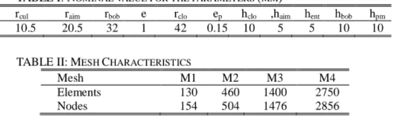
mobile plate, when the coil is not energized (due only to the permanent magnet), has been calculated using the Maxwell Stress Tensor. We have fixed nominal values for the parameters pinom (see Table I) and consider an interval of

variation of [0.1pinom,1.9pinom] for each parameter. To account

for the modification of the geometry, the transformation method is used but with always the same mesh. To study the influence of the mesh, we consider 4 meshes Mi with rectangular elements which characteristics are given in Table II. The full model, the error estimation, the POD and (D)EI methods have been programmed under Matlab environment. The feature of the force has been estimated using the finest mesh (see VIII.B). Due to the high range of variation of the parameters, the ratio between the maximum and the minimum of the force is approximately equal to 650. The mean value of the force has been estimated equal to 90 N with a standard deviation of 81 N showing that the dispersion of the force is large. The wide range of parameter values leads to a variation of the discretization error due to a high deformation of the mesh which needs to be controlled.

Symetry axis e_p r_clo rbob r_cul raim e hpm hbob hent h_aim h_clo

Mobile plate (Iron)

Yoke (Iron) Permanent magnet Core (Iron) Coil

Fig.2: Half of the geometry of the magnetic holder and the definition of the parameters (rcul,raim,rbob,e,rclo,ep,hclo,haim,hent,hbob,hpm)

TABLE I: NOMINAL VALUE FOR THE PARAMETERS (MM)

rcul raim rbob e rclo ep hclo ,haim hent hbob hpm

10.5 20.5 32 1 42 0.15 10 5 5 10 10 TABLE II: MESH CHARACTERISTICS

Mesh M1 M2 M3 M4

Elements 130 460 1400 2750

Nodes 154 504 1476 2856

Using the Latin Hypercube method [27], we have generated a sample S of S=1000 parameter sets. If we denote y(p) an output of the model (full or reduced), the mean, the standard deviation and the maximum value of y(p) are estimated using

(8)

always the same sample S by the following expressions: S S S ∈ ∀ ≥ > < − = >= <

∑

∈ ∈ p p p p p p ) y( max(y) y ) ( y S 1 std(y) ) y( S 1 y 2 2 (28)

The output y(p) can be any output of the model like the relative error ε or the force F.

B. Accuracy of the full problem

We have reported in Table III the estimation of the mean, the standard deviation and the maximum of the relative error ε(p) (see (14)). As expected, the mean <ε> of the error tends to zero when the number of elements increases. The standard deviation std(ε) is not equal to zero meaning that the discrepancy due to the discretization varies with the deformation of the mesh due to the parameter variation but we can see that this dispersion decreases when the mesh becomes finer. We have also calculated the relative difference:

) ( F ) ( F ) ( F -) ( F * 2 ) δF( Ω A Ω A p p p p p + = (29)

with FA(p) and FΩ(p) the vertical forces obtained by the two formulations, the statistics are reported in the table IV. As stated below for the error, the mean and the standard deviation of δF tend to zero when the number of elements increases. We can also see a strong correlation between the evolution of the statistics of the relative error ε and of the relative force δF

which ratio is kept almost constant when the number of element increases.

TABLE III: STATISTICS OF THE ERROR

Mesh M1 M2 M3 M4

<ε> (%) 16,3 7.71 4.00 2.61 std(ε) (%) 8.56 4.49 2.50 1.67 max(ε)(%) 64.0 38,6 23.3 16.7 TABLE IV: STATISTICS OF THE FORCE DIFFERENCE δF

Mesh M1 M2 M3 M4

<δF> (%) 12.9 6.29 3.15 1.95 std(δF) (%) 10.6 5.69 3.26 2.25 max(δF)(%) 75.3 46.0 27.6 19.1

C. Accuracy of the POD model

We have applied the procedure proposed in VII.A to determine the snapshots. For each mesh Mi, we have represented the evolution of the criterion αn (see (26)) versus

the iterations of the iterative process in Fig.3. After a fast decreasing, as expected, αn remains close but always greater

than 1. However, for the meshes M1 and M2, αn is always

lower than 1.09 for n greater than 30. It means that the discretisation error is always much greater than the reduction error so no improvement of the reduced model are expected by increasing n. However with the meshes M3 and M4, we can see in Fig.3 that αn fluctuates with maximum values close to

2. In that case the process of enrichment of the snapshots sets

is really profitable in terms of accuracy improvements for the reduced model.

To illustrate the previous point, we have stopped the iterative procedure after n=10, 30, 50, 70 iterations. Like that, for each mesh Mi, we have constructed reduced models with an increasing number of snapshots. We present in Fig.4 the evolution of the ratio between the mean of the error <er> of

the reduced model due the discretisation method as well as reduction method and the error <e> only due to the discretisation. Above n=30, no real improvement of the accuracy of the reduced model derived from M1 and M2 can be noticed for n greater than 30 which is not the case with M3

and M4.

We have also evaluated the quality of the reduced model by calculating the mean <εr> and the maximum max(εr) of the

error εr as well as the maximum of the variation of the force

difference δFr using (27). The results are reported in Fig.5 and

Fig.6 for εr and in Fig.7 for δFr. As expected, the error εr (resp.

the force difference δFr) of the reduced model converges

towards the error ε(resp. the force difference δF) of the FE model. Moreover, if we consider the maximum values of εr

and δFr we can see that there is no real improvement of the

accuracy above n=30 snapshots correlating the fact that it is useless to increase the number of snapshots to improve the accuracy which is bounded by the discretization error of the FE method.

Additionally to that, the additive value of the reduced model appears clearly in Fig.3 because with a small number of degrees of freedom (equal here to the number of snapshots) we can obtain a better accuracy than a FE model. For example, a reduced model derived from M4 with 50 snapshots (<ε>=6.0%) has a better accuracy than the FE model M2 with

504 nodes (<ε>=7.7%) with about ten times less DoF’s. D. Accuracy of the (D)EI method

We have applied the (D)EI method in order to approximate the matrix S(p) and F(p) (see (15)). We have generated two samples of parameter sets of length L equal to 78 and 364 leading to two samples of matrices SA(p) and SΩ(p) and vectors FA(p) and FΩ(p). Applying the (D)EI method on these two samples, we have obtained two approximations of the matrices SADEI,L(p) and SΩDEI,L(p) and the vectors FADEI,L(p)

and FΩDEI,L(p).

To evaluate the quality of the approximation, we have applied the strategy proposed in VII.B by calculating αnDEI(pn)

(see(27)) for each p belonging to Pn (see VII.A). We remind

that e(p) has been already calculated during the construction of the POD approximation and erDEI(p) is calculated using the

reduced model combining the (D)EI method and the POD method (see (24)) which is very fast. In Fig.8, we give values obtained for 70 snapshots for the four meshes when L=78. For most of the snapshots, the ratio is very high proving that the (D)EI approximation is not sufficiently accurate. Moreover, we can see that the finer mesh is the more sensitive.

However, with a longer sample of matrices (L=364), the value of log(αnDEI) is always equal to zero meaning that the

matrix S(p) and the vector F(p) are perfectly interpolated for all the pn. The approximation can be considered as valid in

(9)

approximation is exact, in fact, we have SADEI,364(p), SΩDEI,364(p), FADEI,364(p) and FΩDEI,364(p) which are equal to SA

(p), SΩ(p), FA (p) and FΩ(p) respectively. 1 10 100 0 20 40 60 cr it e ri o nα n Iteration number M4 M3 M2 M1

Fig.3: Evolution of the criterion αn in function of the iteration number

0 5 10 15 20 25 0 20 40 60 R a ti o b e tw e e m m e a n (e r) /m e a n (e ) Snapshot number M4 M3 M2 M1

Fig.4: Evolution of the ratio between the mean of the error of the reduced model <er> and the mean of the error of the FE model <e> in function of the number of snapshots 0 0,1 0,2 0,3 0,4 0,5 0,6 0 20 40 60 80 100 M e a n o f th e r e la ti v e e rr o r ε r Snapshot number M4 M3 M2 M1 FE Model FE Model FE Model FE Model

Fig.5: Evolution of the mean of the relative error εr in function of the

number of snapshots (The last value on the right correspond to the error of the FE model) 0 0,5 1 1,5 2 2,5 0 20 40 60 80 100 M a x im u m o f th e r e la ti v e e rr o r ε r Snapshot number M4 M3 M2 M1 FE Model FE Model

Fig.6: Evolution of the maximum of the relative error εr in function of the

number of snapshots (The last value on the right correspond to the error of the FE model) 0 0,2 0,4 0,6 0,8 1 1,2 1,4 1,6 1,8 0 20 40 60 80 100 M a x im u m o f th e r e la ti v e f o rc e d if fe re n ce δ F r Snapshot number M4 M3 M2 M1 FE Model FE Model

Fig.7: Evolution of the maximum of δFr in function of the number of snapshots (The last value on the right correspond to the relative force difference of the FE model)

0 0,5 1 1,5 2 2,5 3 3,5 4 4,5 5 0 20 40 60 R a ti o b e tw e e m lo g ( α D E I) = lo g (e rD E I/ e D E I) Snapshot number M4 M3 M2 M1 FE Model FE Model FE Model FE Model FE Model FE Model

Fig.8: Values of log(αnDEI(p))=log(erDEI(p)/e(p)) (see (27)) for the 70

(10)

TABLE V: STATISTICS OF THE RELATIVE ERROR ε (%) AND THE RELATIVE FORCE DIFFERENCE δF(%) DoF’s _<ε_> _std(ε ) max(ε) <δF > std(δF) max(δF) Full M4 2700 2.6 1.6 16.2 1.9 2.2 19.0 Reduced 70 4.4 2.0 18.0 2.2 2.0 19.6 Full M3 1400 4.0 2.4 23.3 3.1 3.2 27.0

TABLE VI: AVERAGE RELATIVE COMPUTATIONAL TIMES OF THE CONSTRUCTION AND THE SOLUTION OF THE SYSTEM OF EQUATIONS FOR THE DIFFERENT MODELS (THE REFERENCE IS THE REDUCED MODEL IN THE A FORMULATON)

DoF’s A Ω

Full M4 2700 53.4 70.1 Reduced 70 1.0 1.1 Full M3 1400 16.5 25.1

E. (D)EI POD Model

We consider now the reduced POD-(D)EI model derived from:

-the full model based on the mesh M4,

-Z=70 snapshots obtained with the iterative procedure presented in VII.A based on the proposed error estimator which requires the full model solution 70 times for the two formulations.

-Z’=364 calculations of the stiffness matrix S(p) and source vector F(p) for the two formulations. The application enables to extract automatically, by applying the algorithm given in Fig.1, an expression of the matrix S(p) and the vector F(p) under the form (23) with QAs=QΩs=60 and QAF=1 and QΩF=2.

The quality of the approximation has been checked by the proposed error estimator (see VIII.B).

The statistics of the reduced model have been compared to the statistics of the FE models M4 and M3 by reporting in Table V the relative error ε and the relative force difference

δF. We can see that the reduction process deteriorates the accuracy of the reduced model versus its originate FE model M4 which is inevitable. However, the reduced model derived from the mesh M4 has similar statistics as the FE model M3 but with 20 times less unknowns.

In terms of memory usage, since we have used rectangular elements, the number of entries of the matrix S is equal to 9 times the number of unknowns N. If we account for the source vector F, we have to store 10N terms with the full model. These 10N terms have to be recalculated for each new set of parameters. In the case of reduced model, we have to store the QF matrices of size of S and QR vectors of size of F which

represent approximately 600N terms to store which much higher than the full model however with the (D)EI method only few terms needs to be recalculated in order to reconstruct the reduced model.

We have reported in Table VI the relative estimated computational time to construct and to solve the scalar and the vector potential formulations for the different models taking the computational time of the reduced model in vector potential formulation as reference. We can see that the computational time of the two formulations is almost the same as expected in 2D. The reduced model is more than 16 faster than the FE model M3 with almost the same accuracy.

Finally, the reduced model obtained by the proposed procedure of the construction of the reduced model enables to

increase the computation speed with a control of the different sources of discrepancy. Moreover, the accuracy of the reduced model can be always controlled by using the proposed estimator. The calculation of the error of the reduced model can be also very fast by taking advantage of the (D)EI method decomposition of the stiffness matrices.

IX. CONCLUSION

In this paper, we have introduced an error estimator which enables to evaluate at the same time the discrepancies introduced by the FE, the POD and the (D)EI methods. Using this estimator, it is possible to balance the errors introduced by the three methods. Based on this error estimator, we have proposed a procedure to construct automatically a reduced model based on the POD and (D)EI methods. It has been applied on an example in 2D magnetostatics to illustrate the proposed procedure. The results show that a reduced model with almost the same accuracy as a FE model can be constructed but with 20 times less of unknowns and 16 times faster.

ACKNOWLEDGEMENT

This work has been supported by the foundation Arts et Métiers.

REFERENCES

[1] J. Lumley, A.M. Yaglom and V.I. Tatarski “The structure of inhomogeneous turbulence”, Atmospheric Turbulence and Wave

Propagation.., pp. 221–227, 1967.

[2] L. Sirovich, “Turbulence and the dynamics of coherent structures”, Q. Appl. Math., vol. XLV(3), pp. 561–590, 1987.

[3] F. Chinesta, P. Ladeveze, E. Cueto, “A short review on model order reduction based on proper generalized decomposition”, Archives of

Computational Methods in Engineering, vol.18, pp. 395-404, 2011.

[4] P. Feldmann, R. W. Freund, “Efficient linear analysis by Pade approximation via Lanczos process”, IEEE Trans. Computer-aided

design of integrated circuits and systems, vol. 14( 5), pp. 639-649, 1995.

[5] Y. Zhai, Analysis of Power Magnetic Components With Nonlinear Static Hysteresis: Proper Orthogonal Decomposition and Model Reduction, IEEE Trans. Mag., vol. 43(5), pp. 1888-1897, 2007. [6] M.N Albunni, V. Rischmuller, T. Fritzsche, B. Lohmann, “Model-Order

Reduction of Moving Nonlinear Electromagnetic Devices”, IEEE Trans.

Mag., vol. 44(7), pp. 1822-1829, 2008.

[7] T. Henneron, S. Clénet, “Model Order Reduction of Non-Linear Magnetostatic Problems Based on POD and DEI Methods”, IEEE Trans.

Mag., vol. 50(2), 2014.

[8] T. Henneron, S. Clénet, “Model order reduction of quasi-static problems based on POD and PGD approaches”, Eur. Phys. J. Appl. Phys., vol. 64(2), 2013.

[9] M.A. Drissaoui, S. Lanteri,; P. Leveque, F. Musy, L. Nicolas, R. Perrussel, D. Voyer, “A Stochastic Collocation Method Combined With a Reduced Basis Method to Compute Uncertainties in Numerical Dosimetry, IEEE Trans. mag., vol. 48(2), pp. 563-566, 2012.

[10] A. Alla, M. Hinze, O. Lass, S. Ulbrich, “Model order reduction approaches for the optimal design of permanent magnets in electro-magnetic machines”, Hamburger Beiträge zur Angewandten Mathematik 2014-23 (2014).

[11] Y. Sato, H. Igarashi, ”Fast Shape Optimization of Antennas Using Model Order Reduction”, CEFC 2014, Annecy, France

[12] S. Clénet, T. Henneron, N. Ida, “Reduction of a Finite Element Parametric Model using Adaptive POD Methods – Application to uncertainty quantification”, IEEE Trans. Mag., vol. 52(3), 2015 [13] M.W. Hess, P. Benner, “Fast Evaluation of Time–Harmonic Maxwell's

Equations Using the Reduced Basis Method”, IEEE Trans. Micro. Th.

(11)

[14] Y. Chen, J.S. Hesthaven, Y. Maday and J. Rodrıguez, “Certified reduced basis methods and output bounds for the harmonic Maxwell’s equations,” SIAM J. Sci. Comput., vol. 32, no. 2, pp. 970–996, 2010. [15] A. Sommer, O. Farle, R. Dyczij-Edlinger, "A New Method for Accurate

and Efficient Residual Computation in Adaptive Model-Order Reduction," CEFC 2014, Annecy, France

[16] S. Burgard, O. Farle, R. Dyczij-Edlinger, "An h Adaptive Sub-domain Approach to Parametric Reduced Order Modeling" CEFC 2014, Annecy, France

[17] M Barrault, Y Maday, NC Nguyen, AT Patera, “An ‘empirical interpolation’method: application to efficient reduced-basis discretization of partial differential equations”, Comptes Rendus Mathematique 339 (9), 667-672, 2004

[18] S. Chaturantabut and D. C. Sorensen, “Nonlinear Model Reduction via Discrete Empirical Interpolation”, SIAM J. Sci. Comput., vol. 32(5), pp.2737–2764, 2010

[19] W. Prager, J.L. Synge, “Approximation in elasticity based on the concept of functions space”, Quart. Appl. Math., 5, pp 261-269, 1947 [20] F. Marmin, S. Clénet, F. Piriou, P. Bussy, “Error Estimation of finite

element solution in non linear magnetostatic 2D problems”, IEEE Trans. Mag., 34(5), pp 3268-3271, 1998

[21] A. Bossavit, “A rationale for edge-elements in 3-D fields computations”,

IEEE Trans. Mag., vol. 24(1), pp. 74–79, 1988.

[22] Nouy, A.; Clément, A.; eXtended Stochastic Finite Element Method for the numerical simulation of heterogeneous materials with random material interfaces, Int. Jour. For Num, Meth. In Eng., Vol. 83(10), pp 1312-1344, 2010

[23] Nouy, A.; Clement, A.; Schoefs, F.; et al. ; An extended stochastic finite element method for solving stochastic partial differential equations on random domains, Comp. Meth. in Applied Mech. and Eng., Vol. 197(51-52), pp 4663-4682, 2008

[24] H. Mac, S. Clénet, J.C. Mipo, Comparison of two approaches to compute magnetic field in problems with random domains, IET Science,

Measurement & Technology, doi: 10.1049/iet-smt.2011.0123, 2012

[25] H. Mac, S. Clénet, J.C. Mipo, “Transformation method for static field problem with Random Domains, IEEE Trans. Mag.,, Vol. 47(5), pp 1446-1449, 2011

[26] H. Mac, S. Clénet, J.C. Mipo, O. Moreau, “Solution of Static Field Problems with Random Domains” , IEEE Trans. Mag., Vol. 46(8), pp 3385-3388, 2010

[27] M. D. McKay, R. J. Beckman and W. J. Conover, “A Comparison of Three Methods for Selecting Values of Input Variables in the Analysis of Output from a Computer Code”, Technometrics, Vol. 21, No. 2, pp. 239-245, 1979