ELASTIC RECONFIGURATION OF BENDING AND TWISTING RODS IN AIR FLOW
MASOUD HASSANI
D´EPARTEMENT DE G´ENIE M´ECANIQUE ´
ECOLE POLYTECHNIQUE DE MONTR´EAL
TH`ESE PR´ESENT´EE EN VUE DE L’OBTENTION DU DIPL ˆOME DE PHILOSOPHIÆ DOCTOR
(G´ENIE M´ECANIQUE) D´ECEMBRE 2016
´
ECOLE POLYTECHNIQUE DE MONTR´EAL
Cette th`ese intitul´ee :
ELASTIC RECONFIGURATION OF BENDING AND TWISTING RODS IN AIR FLOW
pr´esent´ee par : HASSANI Masoud
en vue de l’obtention du diplˆome de : Philosophiæ Doctor a ´et´e dˆument accept´ee par le jury d’examen constitu´e de :
Mme ROSS Annie, Ph. D., pr´esidente
M. GOSSELIN Fr´ed´erick, Doctorat, membre et directeur de recherche M. MUREITHI Njuki William, Ph. D., membre et codirecteur de recherche M. ´ETIENNE St´ephane, Doctorat, membre
DEDICATION
To my loved ones, To my parents who always support me, To my wife, I could not have done it without her.
ACKNOWLEDGMENT
I am truly thankful of my supervisor Fr´ed´erick Gosselin and my co-supervisor Njuki Mureithi, for their incredible support, patience and immense knowledge. During these years, I learned a lot from them and I will appreciate it forever. I deeply believe that they had and they still have a big impact on my life. I could improve many aspects of my thinking and judgment, whether scientific or non-scientific, by learning from them.
I am grateful to bachelor interns, Michael Plante, Diego Altamirano, Pablo Maceira-Elvira, Anthony Salze and Simon Molgat Laurin, whose work helped me during my research. I am also thankful to Benedict Besner, Nour Aimene, Isabelle Nowlan and Martin Cardonne for their technical support. I thank all the professors and students of the Laboratory for Multiscale Mechanics for providing such a scientific, dynamic and friendly atmosphere.
I owe my lovely family for every single accomplishment in my life especially my parents Dr. Mohammad Hassani and Akram Ozaee who have dedicated their lives for their children. They are the most important reason behind my success because of their unconditional support and love. They mean the world to me.
I have had an amazing support from my love, Elham Kheradmand Nezhad. During my doctoral studies, we had and we continue to have a great and adventurous life together. This always gives me a great motivation and energy to work harder. I am deeply grateful for her support and kindness.
R´ESUM´E
Les plantes sont g´en´eralement flexibles et se d´eforment significativement lorsqu’elles sont soumises `a un ´ecoulement a´erodynamique. Ce changement de forme, qui g´en´eralement r´e-duit la traˆın´ee, est appel´ee reconfiguration. Plusieurs ´etudes dans la litt´erature ont apport´e une compr´ehension fondamentale de la reconfiguration des plantes en la mod´elisant comme une poutre en flexion. Bien que cette approche permette de capturer l’essence de la fl`eche bidimensionnelle des plantes, leur fl`eche tridimensionnelle est ignor´ee. En effet, en raison de leur structure fibreuse, les plantes se tordent significativement sous un ´ecoulement, montrant une reconfiguration tridimensionnelle. De plus, de nombreuses plantes ont une morphologie chirale, ce qui induit une fl`eche tr`es complexe. Le pr´esent travail de recherche vise `a ´etudier l’effet de la torsion et de la chiralit´e dans la reconfiguration des plantes en combinant exp´e-rimentation et mod´elisation pour comprendre comment une tige ´elastique se plie et se tord avec grande amplitude sous le vent. Pour l’´etude exp´erimentale, des tiges composites sont fabriqu´ees en mousse de polyur´ethane et renforc´ees `a l’aide de fibres de nylon qui apportent un couplage de torsion-flexion `a la structure finale. Pour reproduire une structure chirale, les fibres suivent un patron h´elico¨ıdal le long dans la tige. Afin d’enrichir l’´etude exp´erimentale, des rubans chiraux en plastique ABS sont aussi con¸cues. Tous les sp´ecimens sont test´es dans une soufflerie sous diff´erentes conditions d’´ecoulement. Pour l’´etude num´erique, la reconfi-guration tridimensionnelle des tiges et des rubans sera simul´ee utilisant la th´eorie de tiges de Kirchhoff coupl´ee avec une formulation semi-empirique pour introduire les forces a´erody-namiques. Les r´esultats de ces ´etudes montrent que ces structures, fortement anisotropes, se tordent pour ensuite fl´echir selon la direction de moindre rigidit´e en flexion. De plus, la reconfiguration tridimensionnelle d’une tige peut ˆetre caract´eris´ee par une flexion bidimen-sionnelle en choisissant le bon ensemble de param`etres adimenbidimen-sionnelles. Il est aussi constat´e que les rubans chiraux font face `a un compromis, en fonction la configuration g´eom´etrique, entre la r´esistance au flambage plus ´elev´e mais aussi le moment de flexion plus ´elev´e `a la base. Finalement, la chiralit´e rend la fl`eche de ces structures moins d´ependante de la direction de chargement.
ABSTRACT
Plants are generally flexible and deform significantly when subjected to flow. This defor-mation which generally leads to a drag reduction is termed reconfiguration. Fundamental understanding of this phenomenon has been sought by modeling them as bending beams. Although bending beams capture the essence of the two-dimensional deformation of plants, their three-dimensional deformation is ignored. Because of their fibrous structure, plants twist significantly under fluid loading showing a three-dimensional reconfiguration. More-over, many plants are found with a chiral morphology which undergo a complex deformation under loading. The present research aims to model the reconfiguration of plants with an elastic rod undergoing a large deformation, to study the effect of torsion and chirality in reconfiguration. In the experimental investigation, composite rods are made of polyurethane foam and reinforced using nylon fibers which have a bending-torsion coupling. To simulate a chiral structure, the reinforcing fibers are twisted along the length of the rod. Moreover, chiral ribbons are made using ABS plastic. All the specimens are tested in a wind tunnel for a variety of flow and structural properties. The three-dimensional reconfiguration of rods and ribbons is also modeled numerically using the Kirchhoff theory of rods coupled with a semi-empirical drag formulation and the blade element theory. It is shown that a rod with structural anisotropy twists in such a way to bend in its less rigid direction. Moreover, the three dimensional reconfiguration of a rod can be characterized as a two dimensional bend-ing by choosbend-ing the right set of dimensionless parameters. It is found that chiral ribbons face a trade-off between higher self-buckling strength but also higher root bending moment. Moreover, chirality renders the deformation of rods and ribbons less dependent to the loading direction.
TABLE OF CONTENTS
DEDICATION . . . iii
ACKNOWLEDGMENT . . . iv
R´ESUM´E . . . v
ABSTRACT . . . vi
TABLE OF CONTENTS . . . vii
LIST OF TABLES . . . ix
LIST OF FIGURES . . . x
LIST OF APPENDICES . . . xv
CHAPTER 1 INTRODUCTION . . . 1
1.1 Motivation . . . 1
CHAPTER 2 LITERATURE REVIEW . . . 6
2.1 Reconfiguration . . . 6
2.2 Drag Scaling of Natural Structures . . . 7
2.3 Fundamental Investigations on Reconfiguration . . . 9
2.3.1 Dimensionless Parameters in Reconfiguration . . . 9
2.3.2 Two-Dimensional Reconfiguration . . . 11
2.3.3 Three-Dimensional Reconfiguration . . . 13
2.3.4 Similarity in Reconfiguration . . . 14
2.4 Chirality in Natural Structures . . . 16
2.5 Theoretical Framework for Modeling Plants . . . 19
2.6 Biomimetics : Aeroelastic Tailoring . . . 23
2.7 Problem Identification . . . 24
CHAPTER 3 ARTICLE 1 : LARGE COUPLED BENDING AND TORSIONAL DE-FORMATION OF AN ELASTIC ROD SUBJECTED TO FLUID FLOW . . . 26
3.1 Introduction . . . 26
3.2.1 Experimental Procedure and Materials . . . 29
3.2.2 Theoretical Model . . . 33
3.3 Results and Discussion . . . 38
3.3.1 Dimensionless Representation . . . 43
3.3.2 Equivalent Bending Rigidity . . . 46
3.4 Conclusion . . . 51
CHAPTER 4 ARTICLE 2 : BENDING AND TORSIONAL RECONFIGURATION OF CHIRAL RODS UNDER WIND AND GRAVITY . . . 53
4.1 Introduction . . . 53
4.2 Methodology . . . 54
4.2.1 Experimental Procedure and Materials . . . 54
4.2.2 Theoretical Model . . . 56
4.3 Results and Discussion . . . 61
4.3.1 Mathematical Model Verification . . . 61
4.3.2 Buckling . . . 62
4.3.3 Drag and Lift Coefficients . . . 62
4.3.4 Drag of Flexible Specimens . . . 63
4.3.5 Curvature and Bending Moment . . . 65
4.4 Concluding Remarks . . . 69
CHAPTER 5 DETAILS OF EXPERIMENTS . . . 72
5.1 Specimen Fabrication . . . 72
5.2 Bending and Torsional Rigidity . . . 73
5.3 Drag of Rigid Specimens . . . 75
5.4 Details of Wind Tunnel Tests . . . 75
5.5 Static Bending Test . . . 79
5.6 Details of Measurements on Cattail Leaves . . . 79
CHAPTER 6 GENERAL DISCUSSION . . . 81
CHAPTER 7 CONCLUSION . . . 83
7.1 Contribution . . . 83
7.2 Limitations and Future Work . . . 85
REFERENCES . . . 87
LIST OF TABLES
Table 2.1 The average of twist-to-bend ratio for some natural structures . . . 15 Table 2.2 The Vogel exponent for some flexible structures, aquatic and terrestrial
organisms . . . 16 Table 2.3 A comparison between advantages and disadvantages of three different
representations of the material frame . . . 21 Table 3.1 The average of twist-to-bend ratio for some natural and engineering
structures . . . 28 Table 3.2 Physical properties of tested specimen . . . 31 Table 3.3 The Vogel exponent for a range of angle of incidence calculated from
the experimental data points and the mathematical simulation of R3 . 45 Table 4.1 Physical properties of tested specimens . . . 56 Table 4.2 Physical properties of study cases . . . 68
LIST OF FIGURES
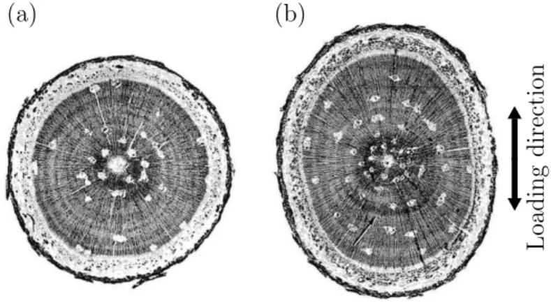
Figure 1.1 The effect of wind on plants. (a) Lodging of crops caused by severe storm (Thomison, 2011). (b) Permanent change in the shape of a tree due to the wind and gravity as known as “flag tree” (Geoff, 2009) . . . 3 Figure 1.2 Demonstration of the effect of mechanical perturbation on the trunk
of loblolly pine. Transverse section of trunk (a) under controlled condi-tions and (b) under mechanical stress (Telewski and Jaffe, 1981) . . . . 4 Figure 2.1 Main mechanisms of drag reduction and reconfiguration. a) An
unde-formed tulip tree leaf and b) the leaf reconfiguring in wind by reduction of the frontal area and the drag coefficient. b) Measurements on the crown of black cottonwood which show the reduction of the frontal area and the drag coefficient due to reconfiguration (Vollsinger et al., 2005). The image of the leaf is adapted from Vogel (1989). . . 8 Figure 2.2 Comparison between the drag scaling of a flexible plant (giant reed)
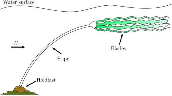
with its equivalent rigid body. Data is obtained from Speck (2003). . . 8 Figure 2.3 A schematic of giant kelp showing its stipe, clumped blades and the
holdfast. The figure is reproduced from Johnson and Koehl (1994). . . 9 Figure 2.4 Different modes of reconfiguration of the London plane tree leaf in
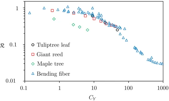
different wind speeds to reduce the drag force and to make it more stable. The unit of velocity is ms−1. Images are obtained from Shao et al. (2012). . . 10 Figure 2.5 The variation of the reconfiguration number with the Cauchy number
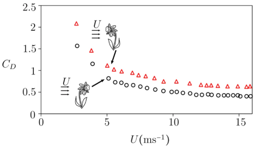
for different natural species (de Langre, 2008) compared with a fiber bending in flow (Alben et al., 2002). . . 12 Figure 2.6 Comparison between the drag coefficient of a Daffodil flower facing
downwind and upwind. Data has been extracted from Etnier and Vogel (2000). . . 14 Figure 2.7 Similarity of simple mechanical structures with natural ones by
com-paring a) a palm tree with b) a poroelastic ball, and c) a tulip tree leaf with d) an elastic circular sheet which rolls up. The image of the palm tree is taken by Verdier (2003). The image of the poroelastic ball is extracted from Gosselin and de Langre (2011) and the others are reproduced from Schouveiler and Boudaoud (2006); Vogel (1989). . . . 16
Figure 2.8 Similar trend of experimental results of different specimens subjected to flow and characterized by the reconfiguration number and the sca-led Cauchy number for cut disks △ and a bending rectangular plate ◯ (Gosselin et al., 2010), poroelastic ball × (Gosselin and de Langre, 2011), circular flexible plate which rolls up in flow ◇ (Schouveiler and Boudaoud, 2006) and bending fibers ◻ (Alben et al., 2004). The line represents the mathematical model for the two-dimensional reconfigu-ration of a plate in flow (Gosselin et al., 2010). Images are extracted from the mentioned references. . . 17 Figure 2.9 a) a carbon nanotube rope with a chiral morphology (Zhao et al., 2014)
and b) a chiral cattail leaf . . . 18 Figure 2.10 A rod connected to a fixed coordinate system with moving material
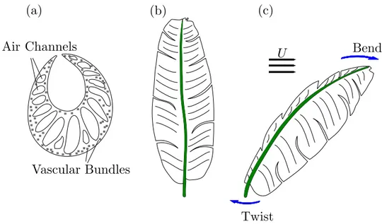
frames connected to its centerline. . . 20 Figure 3.1 Schematics of a banana leaf (a) U-shape cross section of its petiole
with a large twist-to-bend ratio ; (b) upright banana leaf ; and (c) leaf twisting to bend downwind. Inspired by Ennos et al. (2000). . . 29 Figure 3.2 Schematic of the test setup installed on top of the wind tunnel. The
setup consists of a servo (1), gearbox (2), force balance (3), aluminum frame (4), wooden panel (5) and a rod specimen (6). . . 30 Figure 3.3 Photograph of a flexible rod’s section made of polyurethane foam and
reinforced with nylon fibers which have an angle of incidence ψ with the flow. The angle of incidence at the clamped end is defined by ψ0. . 32
Figure 3.4 Schematic of a rod connected to a fixed coordinate system with moving material frames attached to its centerline. . . 34 Figure 3.5 Photographs of deformed shapes of the specimen R3. Thin lines
re-present the deformation of an equivalent rod predicted by the mathe-matical model. The velocity unit is ms−1. . . 40 Figure 3.6 Mathematical evaluation of the in-plane and out-of-plane deformation
of specimen R3 for three angles of incidence by showing a) the variation of the tip’s X-component, b) the tip’s Y -component and c) the tip’s Z-component with flow velocity. Some experimental data points are provided for reference as markers. Error bars represent the standard deviation of the time fluctuations of the tip position. . . 42
Figure 3.7 Time-averaged drag of the specimen R3 for a range of ψ0 from 0○ to
90○. Drag loading on an equivalent rigid rod is provided as a line for reference. Error bars represent the standard deviation of the time fluc-tuations for series ψ0 = 45○. Time fluctuations are similar for other
series. . . 43 Figure 3.8 Twisting moment at the root of the specimen R3 varying by the flow
velocity and angle of incidence. The mathematical evaluation of the root’s twisting moment is provided as lines for reference. . . 44 Figure 3.9 Experimental drag scaling of the specimen R3 represented by the
Cau-chy number and the reconfiguration number. The equivalent mathema-tical model for ψ0 = 0○, 45○ and 90○ is provided as lines. . . 45
Figure 3.10 The reconfiguration number of the three specimens (table 3.2) for a range of ψ between 0○ and 90○ plotted versus a) the Cauchy number and b) the equivalent Cauchy number to find a generic representation of the drag scaling. The Mathematical models for ψ0 = 0○ and ψ0 = 90○
are presented as lines. . . 48 Figure 3.11 Mathematical demonstration of torsion of R3 along its length by
plot-ting the variation of ¯τ with ¯s, CY∗ and ψ0. . . 50
Figure 3.12 Experimental evaluation of the torsion length of specimen R3 varying with the equivalent Cauchy number. The mathematical model is pro-vided as lines for comparison. . . 51 Figure 4.1 a) Schematics of chiral rods with an intrinsic twist angle varying from
0○to 360○as well as a real rod specimen. b) Schematics of chiral ribbons with an intrinsic twist angle varying from 0○ to 360○ a well as a real twisted ribbon. c) Section of a chiral rod and d) section of a chiral ribbon both with an incidence angle of ψ. e) Schematic of a chiral ribbon deformed in the flow with a moving material frame attached to its centerline. . . 56 Figure 4.2 a) Static bending test for chiral circular rods. The rods are fixed
hori-zontally from one end and their maximum vertical deflection is plotted vs. the angle of incidence at the fixed end. Markers represent the ex-perimental results. b) The effect of chirality and the bending rigidity ratio of rods on their critical buckling length. . . 63
Figure 4.3 Rose plot of drag as a function of the intrinsic twist angle, τ0 and the
incidence angle, ψ for a) chiral circular rods with U = 13 ms−1 and b) chiral ribbons with U = 15 ms−1. c) Maximum and minimum relative drag of chiral circular rods at U = 13 ms−1 and d) chiral ribbons at U = 15 ms−1 among a range of incidence angles. Markers represent the experimental data and lines show the mathematical prediction. The maximum and minimum drag of equivalent rigid rods and ribbons are also provided for reference. . . 66 Figure 4.4 Theoretical evaluation of the deformed shape of weightless ribbons
un-der a terminal moment with a)τ0 = 0○ and b)τ0 = 360○. Deformed
shape of upright ribbons under the wind loading with c)τ0 = 0○ and
d)τ0 = 360○. Contour of the total curvature κt for e) weightless chiral
ribbons under a terminal moment and f) upright ribbons in the flow. The terminal moment is ¯MY = 1.2, the Cauchy number is CY = 30 and
ψ0 is null for all cases. Small arrows show the curvature nodes on the
deformed ribbons. . . 67 Figure 4.5 Maximum dimensionless bending moment at root of five study cases at
CY = 30. Plots are predicted using the mathematical model. The
sha-ded area represent the range of the most probable intrinsic twist angle of the cattail specimens collected for this study. The small histogram plot shows the distribution of the collected specimens in terms of the intrinsic twist angle. . . 70 Figure 5.1 Photograph of the mold used to fabricate circular rods. . . 72 Figure 5.2 Schematic of the test setup used to measure the torsional rigidity of
a rod. In this test setup, the rod (1) is attached to the center of a rectangular aluminum plate (2) which can rotate around a pin (3) freely. The pin limits the movement of the aluminum plate to rotation around its center. . . 74 Figure 5.3 Wind tunnel measurements of the lift and drag coefficients of a metallic
ribbon equivalent to flexible ABS ribbons averaged over Re= 10000 and Re= 20000. Markers represent experimental values and lines are fitted trigonometric functions (Eq. (4.36) and Eq. (4.37)). . . 76
Figure 5.4 Variation of a) the lift and b) the drag coefficients for a rigid chiral ribbon with τ0= 90○ as a function of the incidence angle ψ0. The length
and width of the ribbon are 400 mm and 25.4 mm respectively. Lines re-present the mathematical model for two different thicknesses. Symbols represent the experimental results for two different Reynolds numbers. 77 Figure 5.5 a) Photograph of the mast used for testing circular rods. It consists of a
circular adapter for connection to the force transducer (1a), an acrylic rod (2a), a sleeve (3a) and a threaded hole to hold the M4 screw of circular rods (4a). b) Photograph of the mast used for testing ABS ribbons. It consists of a circular adapter for connection to the force transducer (1b), an acrylic rod (2b), a slot (3b) and a threaded hole to keep ribbons in place (4b). Small ellipses at the end of masts represent the reference point schematically. . . 78 Figure 5.6 Test setup for the static bending test showing a cantilever rod (2)
deforming under its own weight. The rod is attached to a disk (1) which can be rotated around its center to impose different incidence angles. The definition of the incidence angle is shown at the lower left of the figure. . . 79 Figure 5.7 Photograph of cattail leaves at the the Voyageur Provincial Park in
LIST OF APPENDICES
CHAPTER 1 INTRODUCTION
Mechanical engineering structures are typically rigid and do not deform significantly under loading. In contrast, plants are flexible and deform with large amplitude when subjected to fluid flow and gravity. The deformation of plants under fluid loading can be very large leading to structural failure. This phenomenon is generally known as “wind damage” which has adverse effects on human life. Moreover, mechanical stresses exerted by fluid loading can permanently alter the structure of plants and change their geometry and growth rate. These phenomena have motivated numerous studied on the deformation of plants in nature. Many types of plants have been tested to study their interaction with fluid flow. Furthermore, fundamental understanding of the deformation of plants in flow has been undertaken by modeling them as simple structures such as bending beams and plates. This has led to better understanding the underlying mechanisms of deformation and the drag reduction of plants in nature.
While simple bending structures cover the essence of the deformation of plants, their twisting mechanism is ignored. Moreover, many plants have geometrical complexities which cannot be studied using a simple bending beam. In this research, we simulate the arbitrary large deformation of plants using an elastic rod model. A rod is a slender beam capable of having a torsional deformation in addition to the bending deformation. Our goal is to understand the deformation mechanisms of plants in the presence of torsion. We evaluate the effect of torsion in the drag scaling of plants as flexible structures. To do this, a mathematical model for an arbitrary deformation of rods is developed and wind tunnel tests are performed. In the next section, the motivation behind this study is discussed. This is followed by an exploration of the existing knowledge in the field. The main questions of the present research are then precisely defined.
1.1 Motivation
The destructive effects of wind and water flow on plants including windthrow, uprooting and lodging (see Fig. 1.1a) are a big concern around the world since they have many adverse effects on human life. Wind damage to trees causes severe environmental changes in forests and affects the regeneration of trees (Ulanova, 2000). In addition, human injuries, road blockage, power outage and the reduction of construction materials are examples of problems linked with windthrow. Lodging can cause an 80 percent reduction in the crop production in addition to making harvesting more difficult and decreasing the quality of the products (Berry et al.,
2004).
In recent decades, many approaches have been developed to predict the response of individual plants or plants in a canopy to flow. In order to evaluate the drag force and the uprooting strength, it is necessary to consider several parameters such as the plant’s height, diameter and stiffness as well as soil strength. There exist software packages such as HWIND (Peltola et al., 1999) and ForestGALES (Gardiner et al., 2000) which can calculate the critical wind speed or snow loading needed to damage or uproot some types of trees like pine and spruce. These packages take the geometry of trees in a canopy, spacing between them, wind speed and material properties to calculate the risk of wind damage and the critical wind speed. They use a simple mathematical model considering an average wind speed and drag coeffi-cient, to evaluate the root moment without considering the deformation of trees. Researchers have also developed mathematical models to predict the risk of lodging of cereals using the aforementioned parameters (Baker et al., 1998; Berry et al., 2003, 2006). In addition, theories and mathematical models have been established to study the strategy of plants to withstand large deformations with an optimized structural mass (Pasini and Mirjalili, 2006; Brul´e et al., 2016) and increase their buckling stability (Speck et al., 1990; Spatz et al., 1990; Burgess and Pasini, 2004).
The prediction and control of wind damage has made it possible to decrease the occurrence of tree failure and crop lodging in recent decades by applying proper field management and genetic or chemical manipulation. For instance, between the 1960s and 1970s, many efforts were made to alter crops to generate smaller varieties known as dwarf or semi-dwarf which were more resistant to lodging. As a result, cereal yields have been increased by 0.5 to 1 ton per hectare each decade in many countries in Asia, Europe and North America. These methods are now used around the world. For example, in France, the United Kingdom and Germany which are among the top grains producers in the world, these manipulations are applied to more than 70 percent of the wheat fields (Berry et al., 2004).
Wind damage is intrinsically a fluid-structure interaction problem. The main fluid force acting on plants is the drag force. In the aforementioned failure risk evaluation models, a constant drag coefficient is considered to calculate the wind loading on plants. In general, these models use an empirical value for the drag coefficient which is obtained experimentally. They mainly focus on limited types of trees and crops and cannot be generalized to all types of plants. In general, plants have long slender structures e.g. trunks, petioles and stems. In engineering, beams are long and slender structures therefore we can model plants as elastic beams defor-ming in flow. This approach is advantageous over testing each species of plants separately because it is simple and reproducible. Using a beam model, we can fundamentally investigate
(a) (b)
Figure 1.1 The effect of wind on plants. (a) Lodging of crops caused by severe storm (Tho-mison, 2011). (b) Permanent change in the shape of a tree due to the wind and gravity as known as “flag tree” (Geoff, 2009)
the deformation of plants under fluid loading.
Wind can cause permanent changes in the plant shape.“Flag tree” is a graphic example as shown in Fig. 1.1b. Wind also affects plant growth through what is known as “Thigmomor-phogenesis” (Niklas, 1998). Environmental conditions such as fluid loading, sunlight direction or external mechanical stresses such as gravity, lead to the production of chemicals in plants which alter their growth rate and stiffness. For example, sugar maple trees from open and windy sites have smaller and more flexible leaves than those from wind protected sites (Nik-las, 1996). The change in the growth rate under the mechanical perturbation is illustrated in Fig. 1.2 which shows that radial growth rate increases in the direction of the applied per-turbation. This means that plants adapt themselves to external loading and their growth rate increases where the load is applied (Mattheck and Bethge, 1998; Mattheck et al., 2003; Mattheck, 2006). As another example, Telewski and Jaffe (1986a,b) report an increase in radial growth rate and a decrease in the flexibility of loblolly pine and fraser fir induced by mechanical perturbation. This is also observed in aquatic plants. For instance, the rigidity and consequently the canopy height of eelgrass is strongly affected by the magnitude of water flow (Abdelrhman, 2007). Moreover, experiments on giant kelp show that species which live in fast moving water flows have narrower blades with lower drag, preventing structural failure (Koehl and Alberte, 1988; Johnson and Koehl, 1994).
The interaction between plants and fluid flow is inspiring in engineering. Plants are able to passively extend their stability envelope and decrease the mechanical loading on their
structure by being flexible. This can be used to address several problems in mechanical and aerospace engineering where the interaction between fluid and structure is important. For instance, to improve the mission adaptability and stability of micro aerial vehicles (MAVs), extremely flexible rotor blades are considered which undergo a large amplitude of deformation (Sicard and Sirohi, 2012, 2014, 2016). A wind turbine can be designed to cone passively in high winds to cope with the excessive wind loading. This means that the turbine blades can bend downwind around a hinge to create a cone-shaped swept area. This concept was originally developed to deal with the bending moment caused by the weight of heavy steel blades. However, modern blades are made of light composites and the concept of coning can be used to increase their operational wind speed range. Wind turbines are commonly designed for wind speeds up to 15 ms−1 (Jamieson, 2011). By implementing the passive coning mechanism, fluid loading on the blades can be reduced in high winds to avoid structural failure (Curran and Platts, 2006).
Passive adaptive wind turbine blades based on the concept of aeroelastic tailoring are also an example of adaptation to the flow. These blades are used to bypass extreme loading (Lago et al., 2013). Aeroelastic tailoring can also be used to build adaptive rear wings for Formula 1 cars. This type of rear wing is able to create high downward forces at low speeds and low drag force at high speeds (Thuwis et al., 2009). Moreover, it can be applied to flexible wings to create high lift-to-drag ratio and increased stability (Stanford et al., 2008; Ifju et al., 2002) and flexible marine propellers for improved performance (Liu and Young, 2009).
The aforementioned applications can be modeled as flexible structures interacting with the flow. Understanding the underlying mechanisms of deformation of these structures by means of mathematical modeling can therefore reduce the production cost and increase the reliability
(a) (b) L oa d in g d ir ec tio n
Figure 1.2 Demonstration of the effect of mechanical perturbation on the trunk of loblolly pine. Transverse section of trunk (a) under controlled conditions and (b) under mechanical stress (Telewski and Jaffe, 1981)
of design (Lago et al., 2013). The mathematical modeling can also be applied to engineering applications dealing with slender structures bending and twisting under a loading other than a fluid force. An example of this case is a soft actuator made of a shape memory alloy which twists and bends by applying an electric current (Shim et al., 2015). Many of these engineering components can be modeled as flexible beams and rods deforming under external forces and torques. Therefore, in this research we aim to develop a generic mathematical framework capable of modeling the complex deformation of plants and slender structures under external loading.
CHAPTER 2 LITERATURE REVIEW
In this section we review the existing knowledge on the experimental and theoretical modeling of plants and slender structures interacting with the flow.
2.1 Reconfiguration
In contrast to mechanical structures, plants are flexible and deform significantly under fluid loading. This deformation which usually leads to a drag reduction is termed “reconfiguration” in the literature (Vogel, 1984, 1989). The drag force D of a rigid bluff body is proportional to U2 where U is the flow velocity. However, plants are subjected to a drag which is not
proportional to the square of the flow velocity. As suggested by Vogel (1984), the reconfigu-ration of different natural species may be compared by studying their divergence from the drag scaling of rigid bluff bodies. To do this, he introduces the Vogel exponent ϑ as the slope of the logarithmic plot of D/U2 or “speed specific drag” versus the flow velocity. The drag
force on flexible structures is proportional to U2+ϑ :
D∝ U2+ϑ . (2.1)
The Vogel exponent ϑ quantifies the effect of reconfiguration in the drag velocity relation. For rigid bluff bodies, ϑ is null since they do not reconfigure. Conversely, for flexible struc-tures, ϑ is generally negative. The more negative ϑ is the more the drag reduces due to the reconfiguration.
There are two main mechanisms of reconfiguration although the deformation of natural flexible structures in the flow is complex. In general, the drag force is proportional to the drag coefficient and the frontal area therefore decreasing these two parameters, reduces the drag force. For instance, Fig. 2.1a shows an undeformed tulip tree leaf and Fig. 2.1b shows the leaf reconfiguring in wind by rolling around itself. This reduces the wind loading by decreasing the frontal area and by streamlining which is equivalent to the drag coefficient reduction. Flexible plants use these two mechanisms to reduce the pressure drag, but the effect of each method on the reduced drag is different depending on the plant. For example, Fig. 2.1c shows measurements of the drag coefficient and the frontal area for the unpruned crown of black cottonwood. It illustrates how the drag coefficient and the frontal area decrease with increa-sing wind speed or increaincrea-sing magnitude of deformation. In this plot, the drag coefficient is calculated using the still-air frontal area, therefore it only represents the effect of streamlining
(Vollsinger et al., 2005).
2.2 Drag Scaling of Natural Structures
Researchers in the fields of biology, botany and forestry, have worked on the deformation and the drag scaling of plants, terrestrial and aquatic vegetation. They have studied passive methods which plants employ to cope with the wind and water loading. Observing flexible structures in nature, they came up with the following question : what is the effect of fluid flow on plants ? To answer the question, many types of plants, crops, algae, leaves and trees were tested individually or in communities in wind tunnels, water canals or their natural habitats to obtain the drag scaling. The results show that the drag scaling of natural flexible structures is different from the drag scaling of rigid bodies (Vogel, 1984). For instance, Fig. 2.2 shows the drag scaling of a giant reed, a flexible slender and upright plant, measured by Speck (2003). Comparison is made with the drag of an equivalent rigid bluff body which follows the curve of U2. In the figure, the drag force on the flexible giant reed follows the drag force of
the rigid body at low wind speeds but starts to diverge from this scaling on increasing the flow velocity.
Many types of aquatic plants and algae have flexible structures and reconfigure in water flow. Giant kelp or mermaid’s bladder as an example, is a kind of kelp which grows in the cold waters of the American Pacific coast. It has a long stipe which is attached to a float and blades. Also, a holdfast keeps this plant attached to the substrate as shown in Fig. 2.3. Observations show that the giant kelp bends in water flow and also clumps its blades. This reduces its frontal area and makes it more streamlined which decreases the drag force on its structure (Koehl and Alberte, 1988; Johnson and Koehl, 1994). Because of the gas filled float in the plant, a buoyancy force acts in addition to inertial and hydrodynamic forces (Koehl, 1977).
In addition to aquatic plants, researchers have studied many types of terrestrial species such as crops, trees and leaves in wind tunnels or in open sites to obtain their drag scaling and observe their reconfiguration. In this context, studies have been done on tree crowns (Rudni-cki et al., 2004; Vollsinger et al., 2005), crops (Sterling et al., 2003) and leaves (Vogel, 1989) in wind tunnels or their natural setting to understand the effect of the streamlining and the frontal area reduction on their drag scaling. Researchers have also investigated the dynamical behavior of plants experimentally for terrestrial (Rodriguez et al., 2012) and aquatic plants (Abdelrhman, 2007) or theoretically for trees (Saunderson et al., 1999; Spatz et al., 2007) and grasses (Br¨uchert et al., 2003; Speck and Spatz, 2004), studying for instance the damped oscillations of plants. Reconfiguration is found to be a method to make plants stable and to
(a)
(b)
(c)
Projected Area Drag CoefficientA
(m
2)−
C
D 0 0 5 10 15 20 0.2 0.4 0.6 0.8U
(ms
−1)
Figure 2.1 Main mechanisms of drag reduction and reconfiguration. a) An undeformed tulip tree leaf and b) the leaf reconfiguring in wind by reduction of the frontal area and the drag coefficient. b) Measurements on the crown of black cottonwood which show the reduction of the frontal area and the drag coefficient due to reconfiguration (Vollsinger et al., 2005). The image of the leaf is adapted from Vogel (1989).
reduce the chance of structural failure due to flutter. For example, edges of the London pla-netree leaf curl to form a structure similar to a delta wing which can reduce the wind-induced vibrations and stabilize the leaf. With increasing wind speed, the leaf rolls up and becomes more stable in different modes of reconfiguration. Figure 2.4 shows the reconfiguration of a London planetree leaf in the wind tunnel for different wind speeds. In this experiment, the Reynolds number is in the range of 104 to 105 (Shao et al., 2012).
0
0
4
6
8
10
1
2
2
3
Giant reed
Rigid body
U
(ms
−1)
D
(N)
Figure 2.2 Comparison between the drag scaling of a flexible plant (giant reed) with its equivalent rigid body. Data is obtained from Speck (2003).
Water surface
Blades
Holdfast
Stipe
U
Figure 2.3 A schematic of giant kelp showing its stipe, clumped blades and the holdfast. The figure is reproduced from Johnson and Koehl (1994).
2.3 Fundamental Investigations on Reconfiguration
In the preceding sections, studies on the reconfiguration of plants whether aquatic or ter-restrial were reviewed. These studies mainly deal with trees, algae, leaves and flowers. In general, plants have greater material and structural complexity in comparison with enginee-ring structures. They have complex geometries, they are not identical and they are made of anisotropic materials. Their material properties are also not constant and change with dif-ferent parameters such as moisture content and weather humidity (Glass and Zelinka, 1999). It is therefore difficult to gain a fundamental understanding of the underlying mechanisms of their reconfiguration. To gain this understanding, it is necessary to idealize plants with a simpler structure ignoring geometrical and material complexities and provide a general model which can be applied to different species of plants while giving reproducible results. So far we have seen that plants usually have flexible and slender structures and reconfigure when subjected to flow. One approach to model this phenomenon is to study simple mechanical structures with similar behavior to plants such as flexible beams and plates.
2.3.1 Dimensionless Parameters in Reconfiguration
Due to the diversity of specimens and flow conditions, it is essential to use dimensionless parameters to define the state of the system. The Cauchy number CY is a dimensionless
repre-U
U = 0.7 U = 2 U = 4.8 U = 7
Figure 2.4 Different modes of reconfiguration of the London plane tree leaf in different wind speeds to reduce the drag force and to make it more stable. The unit of velocity is ms−1. Images are obtained from Shao et al. (2012).
sents the ratio of the fluid force to the bending rigidity of the flexible body (Chakrabarti, 2002; de Langre, 2008; Gosselin et al., 2010; Gosselin and de Langre, 2011). The Cauchy number is also called “dimensionless velocity” (Alben et al., 2002, 2004) or “elastohydrody-namical number” (Schouveiler and Boudaoud, 2006). For bending plates and beams fixed at one end, the Cauchy number is defined as :
CY =
ρU2dL3
2EI , (2.2)
where d and L are respectively, the width and the length of the beam or plate. In addition, ρ is the flow density and EI is the bending rigidity.
The reconfiguration number (Gosselin et al., 2010) and similarly the “effective length” (Luhar and Nepf, 2011) demonstrate the effect of flexibility on the drag force which is exerted on a flexible body. The reconfiguration number is defined as the ratio of the drag force on the flexible body to the drag force of an equivalent rigid body with a similar geometry :
R = 1 D
2ρU2CD,rigidA
. (2.3)
The reconfiguration number is a measure of the drag reduction of a flexible structure because of its flexibility. It is suggested by Gosselin et al. (2010) that the reconfiguration number is a function of a constant drag coefficient and the Cauchy number. They define the “scaled Cauchy number” as CYCD; this makes the reconfiguration number a function of the scaled
Cauchy number only.
three different plants and a bending fiber in fluid flow. In all cases the reconfiguration number decreases with increasing Cauchy number. For small Cauchy numbers, the reconfiguration number is near one which means that the deformation of the structure is small. This regime is equivalent to a Vogel exponent of zero. By increasing the Cauchy number, the flexible structure starts to deform therefore its drag scaling diverges from the drag scaling of rigid bodies. This reduces the reconfiguration number. In the large deformation regime where the Cauchy number is large, the drag scaling slope reaches a constant Vogel exponent.
2.3.2 Two-Dimensional Reconfiguration
A flexible beam undergoing bending due to flow is a simple academic representation of re-configuration. For instance, to study two-dimensional reconfiguration of beams, Alben et al. (2002, 2004) tested glass fibers in a very thin layer of soap film to create a two-dimensional flow and be able to visualize the flow. In this experiment, a vertical soap film flow was used with film flow thickness of 1 to 3 µm and flow velocity ranging from 0.5 to 3 ms−1. Thin glass fibers were then used as flexible beams to study two-dimensional reconfiguration. To theo-retically model the bending fiber in the soap film flow, the authors coupled Euler-Bernoulli beam theory with an exact potential flow solution using Helmholtz’s free streamline theory. The free streamline theory is used in this case to account for the wake behind the fiber. In the model, a constant pressure, different from the free stream pressure, is considered for the wake. However they had to introduce an empirical factor to account for the back pressure in the wake. Figure 2.5 shows the experimental drag measurements for a flexible glass fiber in dimensionless form. The Vogel exponent is found to be close to zero for small CY meaning
that the glass fiber acts as a rigid body in this regime. The Vogel exponent reaches −2/3 in the large deformation regime (Alben et al., 2002). As Gosselin et al. (2010) explain in detail, using dimensional analysis, the Vogel exponent can be predicted for large deformation where the initial length scale vanishes. This regime is called the asymptotic condition. In theory, this happens when the flexible structure is fully deformed and aligned with the flow so only a small fraction of the structure near its support produces pressure drag force. The regime of large deformation or asymptotic conditions cannot be reached completely in experiments because of flutter instabilities encountered for high Cauchy numbers. In this regime the initial length scale of the structure loses its role. For bending plates and beams we thus deal with a problem which can be defined by the bending rigidity per unit width, flow velocity, density and the drag force per unit width. According to the Buckingham π theorem (Buckingham,
0.1
0.1
0.01
1
1
10
100
1000
R
C
YTuliptree leaf
Giant reed
Maple tree
Bending fiber
Figure 2.5 The variation of the reconfiguration number with the Cauchy number for different natural species (de Langre, 2008) compared with a fiber bending in flow (Alben et al., 2002).
1914), the following single dimensionless number is sufficient to define the problem : D
d2/3(EI)1/3ρ2/3U4/3 ,
thus by comparing the power of the flow velocity in this dimensionless number with the definition of the Vogel exponent we obtain D∝ U4/3 or equivalently ϑ= −2/3.
Bending plates and cut disks have been modeled theoretically by coupling a semi-empirical drag formulation and the Euler-Bernoulli beam theory (Gosselin et al., 2010). The theoretical model was then solved with the shooting method and Runge-Kutta integration along the beam’s length. It was found that the reconfiguration of an elastic plate deforming in wind is similar to the bending fiber in soap film flow studied by Alben et al. (2002). Experiments on bending plates were also done in a wind tunnel with different geometries and material properties as well as cut disks, all made of transparent covers.
To study flexible aquatic plants, the Euler-Bernoulli beam model and semi-empirical drag formulation were coupled, this time considering the effect of buoyancy (Luhar and Nepf, 2011, 2016). They showed that buoyancy works against the drag force, therefore it delays the reconfiguration compared with a bending beam in wind with no buoyancy effect (Gosselin et al., 2010). It was also found that for a beam bending in the water flow, the Vogel exponent is equal to −2/3 for large deformations ; the same result was previously obtained for bending plates in the wind flow (Gosselin et al., 2010), bending fibers in soap film flow (Alben et al.,
2002) and tapered beams (Lopez et al., 2013).
2.3.3 Three-Dimensional Reconfiguration
Although bending beams and fibers are suitable for modeling the two-dimensional bending of plants, they cannot be used for all forms of reconfiguration. Plants can also twist under fluid loading. The “twist-to-bend ratio” (Vogel, 1992; Faisal et al., 2016) is defined as a dimensionless number denoted by η which is the ratio of the bending rigidity EI to the torsional rigidity GJ :
η= EI
GJ , (2.4)
where E is the Young’s modulus, I is the second moment of area or area moment of inertia, G is the shear modulus and J is the torsional constant. High values of η represent a structure which has a larger bending rigidity in comparison with the torsional rigidity so it can twist more easily than it can bend. The Young’s modulus and the shear modulus are material properties while the second moment of area and the torsional constant are geometrical. For homogeneous and isotropic materials, the Young’s modulus and the shear modulus are linearly related ; E = 2G(1 + ν) where ν is the Poisson’s ratio. However, this linear relationship is not typically applied for plants because their structure is usually inhomogeneous.
Leaves attached to petioles are good examples of twisting structures in nature. For example, the banana leaf has a coupling between the bending and torsional deformation due to a petiole with a hollow U-shape cross section. In this case, the torsional rigidity is less than the bending rigidity giving rise to a twist-to-bend ratio of approximately 70 (Ennos et al., 2000). This causes the leaf to twist easily under the wind loading and consequently to bend in the direction with the lower bending rigidity.
Another interesting example of coupling between twisting and bending in nature is the daffodil flower. The daffodil’s stem holds the flower horizontally and shows a combination of twisting and bending in reconfiguration. It was observed (Etnier and Vogel, 2000) that the daffodil stem has a large twist-to-bend ratio (see table 2.1) so the stem tends to twist to face downwind reducing its drag coefficient as illustrated in Fig. 2.6. The combination of twisting and bending deformation allows the daffodil flower to reduce the wind loading on its structure.
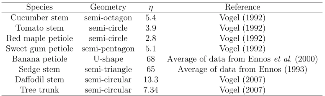
Large values of the twist-to-bend ratio have been observed in many structures in nature. Table 2.1 shows a comparison between the twist-to-bend ratios of some natural structures. In general, structures with a circular or semi-circular sections show a smaller twist-to-bend ratio compared with other section types because of the ratio of I/J (Pasini and Mirjalili, 2006). For comparison, a homogeneous and isotropic circular section has a twist-to-bend
0
0
5
10
15
0.5
1.5
1
2
2.5
U
(ms
−1)
U
U
C
DFigure 2.6 Comparison between the drag coefficient of a Daffodil flower facing downwind and upwind. Data has been extracted from Etnier and Vogel (2000).
ratio equal to 1+ν or 1.5 for materials that maintain their volume in deformation. Also for a metallic circular rod, the twist-to-bend ratio is about 1.3 assuming a Poisson’s ratio of 0.3.
2.3.4 Similarity in Reconfiguration
Figure 2.7a and Fig. 2.7b show the similarity between a palm tree and a poroelastic ball. In both cases, fluid passes through the bodies in addition to flowing around them. Theoretical modeling and experiments on a poroelastic ball consisting of multiple flexible filaments (Gos-selin and de Langre, 2011) shows that in this case, the Vogel exponent varies depending on the density of filaments on the surface. The Vogel exponent is −2/3 for low surface density. This shows that in low surface density where filaments are few, each individual filament is not affected by the surrounding ones and thus acts like a simple bending fiber which leads to ϑ= −2/3. The Vogel exponent reaches −1 for high surface density which has been found for coniferous trees (Vogel, 1984; Rudnicki et al., 2004). This is because of an additional drag reduction mechanism for poroelastic structures which is the reduction of fluid’s effective velocity as it passes through the structure.
Figure 2.7c and Fig. 2.7d show the resemblance between a tulip tree leaf and a circular flexible sheet cut along one radius which rolls up in fluid flow. The reconfiguration of a circular flexible sheet which rolls up in fluid flow was studied by Schouveiler and Boudaoud (2006). In the theoretical modeling, the bending angle of a circular plastic sheet which rolls up in fluid flow was found by minimizing its total potential energy due to the elastic bending and fluid pressure. The fluid pressure on the circular sheet was obtained from an exact solution of the potential flow since viscous effects are negligible for the range of the Reynolds number in
Table 2.1 The average of twist-to-bend ratio for some natural structures
Species Geometry η Reference
Cucumber stem semi-octagon 5.4 Vogel (1992)
Tomato stem semi-circle 3.9 Vogel (1992)
Red maple petiole semi-circle 2.8 Vogel (1992) Sweet gum petiole semi-pentagon 5.1 Vogel (1992)
Banana petiole U-shape 68 Average of data from Ennos et al. (2000) Sedge stem semi-triangle 65 Average of data from Ennos (1993) Daffodil stem semi-circular 13.3 Vogel (2007)
Tree trunk semi-circular 7.34 Vogel (2007)
their experiments. Circular plastic sheets with different size and rigidities were also tested in a water channel. The Vogel exponent was found to be −4/3 in the theoretical model and −1 experimentally.
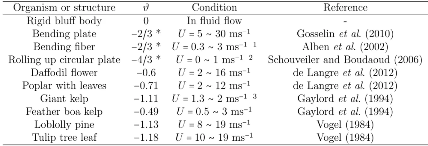
Table 2.2 shows a comparison between the Vogel exponent of a variety of aquatic plants (Gaylord et al., 1994), terrestrial ones (Vogel, 1984; de Langre et al., 2012) and simple struc-tures. This table shows the difference between the reconfiguration of species quantified by the Vogel exponent. Vogel exponents which are marked with an asterisk * are the theoretical values for the asymptotic regime of large deformations where the initial length scale is no longer applicable. Due to instabilities and high level of fluctuations at large deformations, the theoretical Vogel exponent can sometimes not be reached in experiments. All aforementioned flexible structures, from a bending fiber to a poroelastic ball, have different geometries, ma-terials and flow conditions. The goal of the fundamental investigation of flexible structures with similar reconfiguring behavior to plants, is characterizing all these systems similarly. The review of the reconfiguration of some mechanical structures in addition to some species of plants, showed that they have similar reconfiguration characteristics when subjected to flow. For instance, plants with mainly two-dimensional reconfiguration, have a Vogel exponent of around -0.67 which is similar to that of bending beams and plates. As mentioned before, des-pite the differences between plants and simple engineering structures, similar trends are found when their reconfiguration is characterized by the reconfiguration number and the Cauchy number. This similarity is presented in Fig. 2.8 for different flexible structures subjected to fluid flow. In this logarithmic plot, the experimental reconfiguration number for several idea-lized structures as well as the mathematical model for a bending beam is plotted as a function of the Cauchy number. For all cases,R is approximately one for small Cauchy numbers. This
1. In soap film flow 2. In water flow 3. With flat blades
(a) (b) (c) (d)
Figure 2.7 Similarity of simple mechanical structures with natural ones by comparing a) a palm tree with b) a poroelastic ball, and c) a tulip tree leaf with d) an elastic circular sheet which rolls up. The image of the palm tree is taken by Verdier (2003). The image of the poroelastic ball is extracted from Gosselin and de Langre (2011) and the others are reproduced from Schouveiler and Boudaoud (2006); Vogel (1989).
Table 2.2 The Vogel exponent for some flexible structures, aquatic and terrestrial organisms
Organism or structure ϑ Condition Reference
Rigid bluff body 0 In fluid flow
-Bending plate −2/3 * U = 5 ∼ 30 ms−1 Gosselin et al. (2010) Bending fiber −2/3 * U = 0.3 ∼ 3 ms−1 1 Alben et al. (2002)
Rolling up circular plate −4/3 * U = 0 ∼ 1 ms−1 2 Schouveiler and Boudaoud (2006) Daffodil flower −0.6 U = 2 ∼ 16 ms−1 de Langre et al. (2012) Poplar with leaves −0.71 U = 2 ∼ 12 ms−1 de Langre et al. (2012) Giant kelp −1.11 U = 1.3 ∼ 2 ms−1 3 Gaylord et al. (1994) Feather boa kelp −0.49 U = 0.5 ∼ 3 ms−1 Gaylord et al. (1994)
Loblolly pine −1.13 U = 8 ∼ 19 ms−1 Vogel (1984) Tulip tree leaf −1.18 U = 10 ∼ 19 ms−1 Vogel (1984)
means that the amplitude of deformation is very small therefore a flexible structure acts as a rigid structure. Between CY ≈ 1 and 10, depending on the case, the reconfiguration number
starts to diverge from unity and decrease with increasing Cauchy number. This shows that the reconfiguration of these structures is fundamentally similar.
2.4 Chirality in Natural Structures
Many aquatic and terrestrial plants possess a slender structure with a chiral morphology. In mechanical engineering, a chiral structure is a structure which is twisted around its centerline in its natural state. Chirality is also found in organic structures such as DNA (Arbona et al., 2012; Zhao et al., 2015), synthesized ones such as polymers (Ye et al., 2010) and nanoma-terials (Chen et al., 2005; Ji et al., 2012; Zhao et al., 2014). For example, Fig. 2.9a shows a
0.1
0.1
0.01
1
1
10
100
1000
R
C
YC
DU
U
U
U
U
Figure 2.8 Similar trend of experimental results of different specimens subjected to flow and characterized by the reconfiguration number and the scaled Cauchy number for cut disks △ and a bending rectangular plate ◯ (Gosselin et al., 2010), poroelastic ball × (Gosselin and de Langre, 2011), circular flexible plate which rolls up in flow◇(Schouveiler and Boudaoud, 2006) and bending fibers◻ (Alben et al., 2004). The line represents the mathematical model for the two-dimensional reconfiguration of a plate in flow (Gosselin et al., 2010). Images are extracted from the mentioned references.
carbon nanotube rope and Fig. 2.9b shows a cattail leaf both with a chiral morphology. In nature, it seems that upright plants with chirality are less vulnerable to wind loading and buckling (Schulgasser and Witztum, 2004; Zhao et al., 2015; Rowlatt and Morshead, 1992). For instance, Schulgasser and Witztum (2004) show that large twist angles in flat upright leaves can lead to approximately 25 percent increase in the critical buckling length under self-weight loading. Thus, it is concluded that chirality helps upright plants to grow higher than untwisted ones without undergoing structural failure under their own weight. This may be evidence of adaptation of this type of plants to their environment through a long evolution process. The evolutionary aspect of chirality in biological structures has been discussed in many studies. For instance, it is of great interest to know whether the chiral morphology of DNA was a requirement or an outcome of evolution (Lunine et al., 1999) since the chiral morphology of DNA leads to a minimum free energy (Ji et al., 2012).
(a)
(b)
2µm
Figure 2.9 a) a carbon nanotube rope with a chiral morphology (Zhao et al., 2014) and b) a chiral cattail leaf .
Chiral structures have been studied fundamentally using different mathematical models. For example, the Timoshenko beam model has been used to study the dynamics of twisted beams (Chen et al., 2013) and the static stability of chiral upright plants (Zhao et al., 2015). In the latter, the authors use a linear Timoshenko beam theory with a twisted section to model aquatic macrophytes assuming that the beam is linearly elastic with homogeneous and iso-tropic properties. In their buckling analysis, they assume a distributed compressive load along the length of the beam to mimic its weight plus a compressive point force at the free end to simulate a head organ. For the aerodynamic loading, they assume a distributed force which is simply proportional to the projected area of an undeformed beam. Importantly, they assume small deformations. Within their linear framework, they conclude that chirality improves the stability and resistance of upright emergent leaves against high winds and buckling.
To consider large three-dimensional deformations, Kirchhoff theory of rods has been used in several studies related to chirality such as in the behavior of tendrils of climbing plants (Goriely and Tabor, 1998), dynamics of helical strips (Goriely and Shipman, 2000), nanos-prings (da Fonseca and Galv˜ao, 2004), formation of chiral nanomaterials (Wang et al., 2012) and chiral carbon nanotube ropes (Zhao et al., 2014). For example, (da Fonseca and Galv˜ao, 2004) use a classic Kirchhoff rod with intrinsic twist and curvature to study the structural properties of nanosprings. They evaluate the Hooke’s constant of the nanosprings directly from their twist and curvature. Wang et al. (2012) also use a modified Kirchhoff model to take into account the effect of surface stresses. They state that the morphology of quasi-one-dimensional nanotubes is affected by the the surface stress. Despite the vast use of the Kirchhoff rod model, it is not applicable for the problems which involve elongation. To take elongation into account, Wang et al. (2014) develop a Cosserat rod model to study the growth of towel gourd tendrils.
2.5 Theoretical Framework for Modeling Plants
As noted earlier, plants can be modeled as slender flexible structures which bend in fluid flow. However, plants twist and bend simultaneously under fluid loading and their deformation can be very large. Therefore, an appropriate model is necessary to simulate large deformations of slender structures subjected to flow. Euler-Bernoulli beam is a mathematical model which has been used widely to model the deformation of plants (Alben et al., 2002; Gosselin et al., 2010; Luhar and Nepf, 2011). There is also the Timoshenko beam model to include the shear deformation which is ignored in the Euler-Bernoulli beam. However, for structures that are slender enough, the Euler-Bernoulli beam is generally accurate.
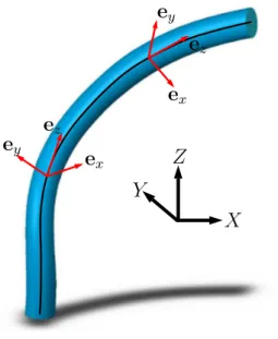
Although the Euler-Bernoulli beam model is simple and convenient, it does not take into account three-dimensional deformation. Therefore, in the present study, we consider the Kir-chhoff model of elastic rods. An elastic rod is a three-dimensional slender structure where its length (L) is much larger than the other two dimensions which make its cross section. Kirchhoff’s theory of rods is a classic theory considering finite displacements while neglecting the shear deformation and assuming small strains (Dill, 1992). In the theory, the rod is re-presented by an “inextensible” curve in three-dimensional space. As detailed by Audoly and Pomeau (2010), to track the twist of the centerline, a “material frame” is defined as a moving coordinate system (ex, ey, ez) attached to the centerline (Fig. 2.10). Based on the Kirchhoff
rod model, it is assumed that ez is tangent to the centerline and remains perpendicular to
the cross section through the rod’s deformation. Without loss of generality, we consider that ey is along the more rigid direction of the cross section. Due to the small strain assumption,
the defined material frame remains orthonormal. This is also called the Euler-Bernoulli hypo-thesis or the unshearable rod assumption. The set comprising the centerline and the material frame is sometimes called the “Cosserat curve” (Audoly and Pomeau, 2010).
For a rod under distributed and point forces, the total applied force is written : F(s) = (∫ L
s p(s
′)ds′) + p(L) , (2.5)
where s is the arclength, p is the distributed loading and p(L) is a point force at s = L. In addition, F(s) is the vector of external forces which is also equivalent to the vector of internal forces at the cross section located at s. Using the principle of virtual work we have :
dM(s)
ds + ez(s) × F(s) + q(s) = 0 , (2.6)
torques in the three directions of the material frame. The Kirchhoff model of rods is usually written as a set comprising Eq. (2.6) and the spatial derivative of Eq. (2.5). These two equations are evaluated for each of the three directions of the material frame which leads to a system of six differential equations. The curvatures around ex and ey are termed κx and
κy, and the twist around ez is termed τ . The material frame is connected to the centerline
of the rod and follows its twist and deformation (Audoly and Pomeau, 2010).
There are several approaches to represent the rotation of the material frame with respect to a fixed Eulerian frame. “Euler angles” are the most common three-parameter representation and are named pitch θ, roll φ and yaw ψ. These angles are related to curvatures and twist using three differential equations (Love, 1944) :
κx= dθ dssin φ− dψ ds sin θ cos φ , (2.7) κy = dθ dscos φ+ dψ ds sin θ sin φ , (2.8) τ = dφ ds + dψ ds cos θ . (2.9)
The state of the rod can be fully defined by coupling these three equations with the Kirch-hoff model of rods. Although the Euler angles are directly identifiable in 3D problems and minimize the number of governing equations of a rod, they have some limitations. Equations
Y
X
Z
e
ye
ye
xe
xe
ze
zFigure 2.10 A rod connected to a fixed coordinate system with moving material frames connected to its centerline.
which relate the Euler angles to curvatures have sine and cosine terms which make them non-linear and difficult to solve. Solving these equations also implies mathematical singulari-ties at specific angles where the determinant of the Jacobian matrix approaches zero. These singularities are discussed in detail by Ang and Tourassis (1987).
Another method to represent the moving material frame is using “quaternions” (Hamilton, 1853). Quaternions form a four-parameter representation of the rotation of the material frame without singularities unlike the Euler angles. According to Euler’s theorem of rotation, the orientation of the material frame can be represented by a single rotation angle Φ about a vector b= (bx, by, bz) (Lazarus et al., 2013). The combination of these four parameters make
a quaternion as : ˜ Q= [bXsin Φ 2, bY sin Φ 2, bZsin Φ 2, cos Φ 2] . (2.10)
The “direction cosines” are another representation of the material frame’s rotation (Love, 1944). They do not have singularities and their equations are linear unlike the Euler angles. They are also conceptually simple while the quaternions are more abstract. Direction cosines are the cosines of the angles between a vector and the three directions forming the fixed coordinate system. Since the material frame and the fixed frame have three directions each, nine direction cosines are needed to define the material frame. Six of the direction cosines are independent and the others can be calculated from these six independent ones. Table 2.3 shows a comparison of the advantages and disadvantages of the three different representa-tions of the material frame presented above. Since singularities should be avoided, the Euler angles are rejected. Direction cosines are chosen over quaternions despite requiring more dif-ferential equations because they are conceptually simple. Direction cosines will be detailed in Chapter 3.
A special case of the deformation of a rod is pure bending under a distributed load. Since the deformation is two-dimensional, the flexible structure acts as a beam. The twist of the material frame is not needed and the beam can be defined by its centerline using Eq. (2.5) and (2.6). In this case, p(s) is the distributed load acting in the bending direction and the bending moment is M(s) = −EIdθ/ds where θ is the bending angle. In addition, the tensile
Table 2.3 A comparison between advantages and disadvantages of three different representa-tions of the material frame
Euler angles Quaternions Direction cosines
Singularity free ✓ ✓
Conceptually simple ✓ ✓
force in the beam is neglected. Simplifying the Kirchhoff equations, one differential equation known as the Euler-Bernoulli beam model can define the state of the bending beam :
EId
3θ
ds3 = p (s) . (2.11)
The present study deals with the deformation of rods therefore the geometry and the ae-rodynamic loading are not constant and change with the state of rod. CFD methods are a possibility to find the aerodynamic loading on deformed rods but these method demand a great computation time. An approximate alternative is to calculate the fluid loading on a flexible structure using the exact solution for inviscid and incompressible flow or the poten-tial flow using the free streamline theory. Since the exact potenpoten-tial flow solution leads to zero drag force, which is known as d’Alembert’s paradox, it is necessary to use Helmholtz’s free streamline theory to predict the separation behind a structure in fluid flow. Using this approach, it is possible to obtain the pressure drag exerted on structures in fluid flow (Sobey, 2000). In the method, the free streamline divides the flow around the body to two regions one of which is the wake behind the body and the other is the inviscid and irrotational flow outside the wake (Alben et al., 2002).
The Finite Element Method and the Finite Difference Method are also candidates to solve problems which include the fluid-structure interaction. These methods have been used in several studies such as a swinging filament in uniform flow (Huang et al., 2007), a flapping filament in a soap film (Zhu and Peskin, 2002), a largely deformed net in water flow (Moe et al., 2010) and a hanging aerial fuel hose (Zhu and Meguid, 2007).
Taylor (1952) suggested a semi-empirical formulation to obtain the drag force on an oblique cylinder in three-dimensional flow. This method can also be used to estimate the drag force on a deformed rod. It was suggested that for the range of Reynolds number Re from 20 to 105, the pressure drag coefficient is approximately constant. For this range, the coefficient of
friction drag normal to the centerline is 4Re−0.5 (Taylor, 1952). Taylor stated that only the normal component of the flow velocity to the cylinder’s centerline contributes to the pressure drag force. This method is preferred in the present work due to its simplicity and will be explained in Chapter 3. The normal drag force on an oblique cylinder is thus calculated as :
pn=
1 2ρU
2A(C
D,psin2θ+ 4Re−0.5sin1.5θ) , (2.12)
where CD,p is the pressure drag coefficient and θ is the local angle between the cylinder’s
centerline and the flow direction. In this equation, the first term is the contribution of fluid pressure and the second term the contribution of the friction drag. The longitudinal force
along the centerline of the deformed rod is due to the friction force along the length of the rod :
pz =
1 2ρU
2A(5.4Re−0.5cos θ.sin0.5θ) . (2.13)
The inviscid dynamic fluid force on a deformed rod can be calculated using slender-body theory (Lighthill, 1960; Schouveiler et al., 2005). According to this theory, the dynamic fluid force is proportional to the curvature of the rod :
Fd= −ρAU2
dθ dscos
2θ . (2.14)
where ρA is the added mass of fluid per unit of length. This force is produced because of the changing of the relative velocity of a body in fluid flow. In the present study, the large deformation of rods will be evaluated by coupling the Kirchhoff rod model with the afore-mentioned semi-empirical drag formulation. In the model, the normal and the longitudinal friction drag in addition to the dynamic fluid force will be ignored because in the present study, they are negligible compared with the normal drag force.
2.6 Biomimetics : Aeroelastic Tailoring
The passive reconfiguration of plants in nature inspires the design and fabrication of flexible wings and wind turbine blades with “morphing capabilities”. This concept is usable in air-planes (Shirk et al., 1986), drones (Ifju et al., 2002; Weisshaar et al., 1998), wind turbine blades (De Goeij et al., 1999) and sport cars (Thuwis et al., 2009). In the context of mor-phing structures, aeroelastic tailoring was developed for aerospace applications to design flexible structures to take advantage of deformation under flow loading. In general, aeroelas-tic tailoring is defined as “the embodiment of directional stiffness (rigidity) into an aircraft structural design to control aeroelastic deformation, static or dynamic, in such a fashion as to affect the aerodynamic and structural performance of that aircraft in a beneficial way” (Shirk et al., 1986). Directional rigidity or asymmetric stiffness (De Goeij et al., 1999) refers to the existence of different bending rigidities in different directions. Using aeroelastic tailoring, the aerodynamic center of the wing’s section can be located behind the shear center (elastic axis or torsional axis) to produce a negative pitching moment which has a stabilizing effect when considering static divergence (Lago et al., 2013). The shear center is a point on the cross section of the body where the applied force does not create torsional deformation.
Aeroelastic tailoring is not limited to the aerospace industry. In fact, directional stiffness can have many applications where flexible structures made of composite materials are used to improve the aerodynamic performance of structures (De Goeij et al., 1999). For example,