Addressing leakage in the EU ETS : Border adjustment or output-based allocation ?

(1)

Addressing leakage in the EU ETS:

Border adjustment or output‐based allocation?

Stéphanie Monjon

1

and Philippe Quirion

23 Abstract

The EU ETS has been criticised for threatening the competitiveness of European industry and generating carbon leakage, i.e. increasing foreign greenhouse gas emissions. Two main options have been put forward to tackle these concerns: border adjustments and output‐based allocation, i.e. allocation of free allowances in proportion to current production. We compare various configurations of these two options, as well as a scenario with full auctioning and no border adjustment. Against this background, we develop a model of the main sectors covered by the EU ETS: electricity, steel, cement and aluminium. We conclude that the most efficient way to tackle leakage is auctioning with border adjustment, which generally induces a negative leakage (a spillover). This holds even if the border adjustment does not include indirect emissions, if it is based on EU (rather than foreign) specific emissions, or (for some values of the parameters) if it covers only imports. Another relatively efficient policy is to combine auctioning in the electricity sector and output‐based allocation in exposed industries, especially if free allowances are given both for direct and indirect emissions, i.e. those generated by the generation of the electricity consumed. Although output‐ based allocation is generally less effective than border adjustment to tackle leakage, it is more effective to mitigate production losses in the sectors affected by the ETS. Keywords: Emission trading, border adjustment, output‐based allocation, competitiveness, carbon leakage

JEL

Q38

1 Corresponding author. Centre International de Recherche sur l’Environnement et le Développement (CIRED), CNRS, Jardin Tropical, 45 bis avenue de la Belle Gabrielle, F 94736 Nogent‐sur‐Marne, France. Tel : 0033 (0)1 43 94 73 99. Email: monjon@centre‐cired.fr.

2

Centre International de Recherche sur l’Environnement et le Développement (CIRED), CNRS , Jardin Tropical, 45 bis avenue de la Belle Gabrielle, F 94736 Nogent‐sur‐Marne, France. Tel: 0033 (0)1 43 94 73 95. Email: quirion@centre‐cired.fr.

3

The authors wish to thank, without implicating, Damien Demailly for his past work on the CASE model, Jean‐Pierre Ponssard for useful comments, Jean‐Louis Moray (Eurofer) for helping with the steel nomenclature, and the Cement Sustainability Initiative for providing some data from the "Getting the Numbers Rights" database. The authors also thank Patrick Criqui and Sivana Mima for the data on marginal abatement cost curves from POLES.

This work is part of the Climate Strategies project "Tackling Leakage in a World of Unequal Carbon Prices" led by Susanne Droege and has benefited from the comments of the participants. Stéphanie Monjon also thanks the Réseau de Recherche sur le Développement Soutenable (R2DS, Région Ile‐de‐France) for its funding.

(2)

1. Introduction

After the results of the last UNFCCC conference in Copenhagen and since the US is unlikely to implement a cap‐and‐trade system in the next years, industry groups in the EU will certainly continue to argue the threat imposed by the European Union Emissions Trading Scheme (EU ETS) against their international competitiveness. The fears of competitiveness losses and of carbon leakage are the main arguments put forward by industry lobby groups against stringent climate policies, and in favour of free allocation of allowances.4 Competitiveness and leakage are also the motivations of border adjustments proposals.

Directive 2009/29/EC, which revises the EU ETS, will be applied from the third period of the ETS, i.e. from 2013 onwards. Changes include a much higher share of auctioning, especially in the electricity sector, and some provisions for limiting carbon leakage. The main one is the continued free allowance allocation to the “sectors or subsectors which are exposed to a significant risk of carbon leakage” (Article 10a‐12). However, the Directive also states that “[b]y 30 June 2010, the Commission shall […] submit to the European Parliament and to the Council […] any appropriate proposals, which may include […] inclusion in the Community scheme of importers of products which are produced by the sectors or subsectors [exposed to a significant risk of carbon leakage] ”. In other words, the Directive mentions, albeit cautiously, a border adjustment (BA) for GHG–intensive imports..

In the US, the Waxman‐Markey bill, which was adopted by the House of Representatives in 2009, includes more concrete provisions. If no international agreement on climate change has been reached by January 1, 2018, the president of the United States is required to set up an “international reserve allowance program.” From 2020 onwards, imports in a covered sector would be prohibited unless the importer has obtained an “appropriate” amount of emission allowances from the international reserve allowance program.5

Hence, the political debate on the competitiveness impact of the ETS, the related carbon leakage and on the most appropriate policies for reducing this impact (if any) is not over. The debate is also still open from an academic point of view: there is disagreement among researchers both on the quantitative importance of leakage and on the effectiveness of the policy instruments proposed to limit leakage and competitiveness impacts (Droege et al., 2009).

Referring to this debate, the objective of this paper is to compare the performances of both alternatives – free allocation and border adjustment – to limit carbon leakage, as well as to mitigate production loss, following the increased ambition of the EU ETS during the third period. We develop a computational framework allowing to represent the European industry at a disaggregated level (cement, aluminium, steel and electricity) and to analyse the design of the different "anti‐leakage" options. Then, we provide a quantitative assessment of the impact of these "anti‐leakage" policies on the activity of the different industries included in the model, compared to a scenario without a climate policy, and to a scenario featuring auctioned allowances without any specific "anti‐leakage" feature.

The results show that the determination of the “best option” depends on the target, i.e. limitation of carbon leakage or mitigation of European production loss, and differs depending on the sector

4

In this context, carbon leakage is defined as the increase in GHG emissions in non‐European countries caused by the implementation of the EU ETS. See Droege et al. (2009) for a deeper discussion about the definition of carbon leakage. 5 Similarly, the cap‐and‐trade bills introduced in the U.S. Senate also include provisions for border adjustments, although with less details. This is the case of S. 1733, the Clean Energy Jobs and American Power Act introduced by Senators Kerry and Boxer on October 23, 2009 (Larsen et al., 2009) and of S. 2877, the Carbon Limits and Energy for America’s Renewal Act introduced by Senators Cantwell and Collins on December 11, 2009. The latter proposes an adjustment for both imports, through a “border carbon adjustment”, and exports, through a “targeted relief fund for exporters” (Larsen and Bradbury, 2010).

(3)

considered as well. This last point emphasises the importance of conducting this kind of analysis using a highly disaggregated model.

This paper is organised as follows: section 2 briefly discusses the previous assessments of carbon leakage and of anti‐leakage options; section 3 presents the different scenarios simulated, while section 4 details the model; finally, section 5 discusses the results; and section 6 will provide conclusions.

2. Carbon leakage and anti‐leakage options: results of previous studies

2.1. Carbon leakage: assessments and main channels

Since the UNFCCC was signed, carbon leakage has become an issue that is regularly discussed and evaluated (for an early reference, cf. Felder and Rutherford, 1993; for recent surveys, cf. Gerlagh and Kuik, 2007, and Droege et al., 2009). Given the global nature of the GHG emissions, carbon leakage can reduce the environmental efficiency of a climate policy if only one group of countries commits to abate their emissions while the others do not, as in the Kyoto protocol. The main indicator of leakage is the ratio between the increase in GHG emissions in non‐Annex I countries and the decrease in GHG emissions in Annex I countries. This ratio is called the leakage rate or leakage‐to‐reduction ratio.6 The variations are calculated for a scenario with the climate policy and a scenario without. The estimated leakage‐to‐reduction ratios in applied models vary considerably, from 2% to 130% (Droege et al., 2009).

Two main channels of carbon leakage have been identified in the literature (Reinaud, 2008a). A first leakage channel, sometimes called “energy‐price‐driven leakage”, goes through the energy markets. That is, climate policies decrease the international prices of oil, gas and coal; hence they increase their use in countries without a climate policy. Another channel, often called “the GHG‐intensive industry” channel, or “competitiveness‐driven” route, is related to competitiveness. For instance, the EU ETS increases the production cost of European producers in GHG intensive sectors, some of which are exposed to international competition. If European producers pass through the cost to consumers, then they may lose some market shares vis‐à‐vis foreign producers. If they do not pass through the cost due to international competition, then the European plants with the highest production cost may become unprofitable and cease operation. In both cases, European industry will lose some market shares in both European and foreign markets, with two main consequences: job losses and an increase in GHG emissions in non‐European countries, i.e. carbon leakage.

Two main parameters explain the wide range of leakage‐to‐reduction ratio estimates. The first is linked to energy‐price‐driven leakage: the ratio decreases with the supply elasticity of fossil fuels (Gerlagh and Kuik, 2007). Specifically, with lower supply elasticity, a given decrease in European fossil fuel demand generates a higher response of fossil fuels price, hence a higher increase in foreign emissions. The second parameter is linked to competitiveness‐driven leakage: the ratio increases with the substitutability between domestic and imported products: see the sensitivity analysis in Bernard and Vielle (2009, Appendix B3).

Two main options to reduce carbon leakage have been assessed with economic models: border adjustments and output‐based allocation. As we shall see, with only two exceptions, these options

6

Michael Grubb (personal communication) recently rightly pointed out that the expression “leakage rate” is sometimes wrongly interpreted as the share of EU emissions (or production) that would “leak” to countries without a climate policy, which is completely wrong. Hence we prefer to use the expression “leakage‐to‐reduction ratio”.

(4)

have not been assessed in the same framework, preventing a systematic comparison of their effectiveness7.

2.2 Border adjustments

A BA is a trade measure designed to level the playing field between domestic producers facing costly climate policy and foreign producers with no or little constraint on their GHG emissions. Border adjustments have been assessed both through partial equilibrium models of a particular industry and through general equilibrium models.

Mathiesen and Maestad (2004) simulate a carbon tax in Annex I, with and without border adjustments, in a global partial equilibrium model of the steel industry. They show that border adjustments tackle leakage very efficiently: a border adjustment based on average specific emissions (i.e. emissions per tonne) in Non‐Annex I countries actually reduces steel production and emissions in Non‐Annex I countries. Consequently the leakage‐to‐reduction ratio becomes negative, falling from 40% without the border tax to ‐31%. Note, however, that setting an export border adjustment at the level of Non‐Annex I specific emissions, which are higher than Annex I specific emissions, constitutes an export subsidy for the average Annex I producer, which seems hardly compatible with the WTO (cf. e.g. Ismer and Neuhoff 2007).

Demailly and Quirion (2008a) also simulate a carbon tax in Annex I, with and without border adjustments, but this time in a global partial equilibrium model of the cement industry. Here again, BAs efficiently tackle leakage: the leakage‐to‐reduction ratio falls from 25% without BA to ‐2% or 4%, depending on the level of the border adjustment assumed. In the first case, production exported from Annex I is completely exempted from the climate policy and imports of cement from the rest of the world are taxed in accordance with the CO2 intensity of cement production in the exporting country. In the second case, exports benefit from a rebate corresponding only to the least CO2 intensive technology available at a large scale (a gas‐fired plant with the highest energy efficiency available), and imports are taxed at the same level.

Peterson and Schleich (2007) specifically examine the economic and environmental effects of a border adjustment imposed on countries outside Annex I, or which did not ratify the Kyoto Protocol. The adjustment is applied to both imports and exports, and to both direct and indirect emissions. The authors discuss their capacity to mitigate the loss in export competitiveness, to neutralise the increased import competition as well as to limit carbon leakage in the whole Annex I. The performances related to the commercial flows differ depending on sectors and countries. For instance, “the [border adjustment] is effective in neutralising the increased import competition for most energy‐intensive sectors in the EU 15”, while “it has little effect on import competitiveness in the rest of European Union (REU)”. This is because the energy‐intensive products of the REU are more carbon intensive and around 90% of all their imports of energy‐intensive products come from other Annex I countries on which no BA is imposed. On the other hand, border adjustment has only a low impact on leakage. This may be explained by the fact that border adjustments cannot prevent leakage from the international energy markets channel. Indeed, in most CGE models, and presumably in this one also, the larger part of leakage occurs through the "energy markets channel" (Burniaux et al., 2008).

Kuik and Hofkes (2009) study the effectiveness of border adjustment for tackling the leakage due to the EU ETS. Their model comprises the following sectors: mineral products, steel, electricity and others. The BA is applied only to imported products and direct emissions. Two variants are examined: the adjustment is based either on the direct CO2 emissions per unit of similar product in the EU, or on the average direct CO2 emissions per unit of production in the foreign (exporting) country. The BAs

7 Admittedly, Meunier and Ponssard (2009) also simulate both options, but applied them in a very different manner: they assess a scenario with auctioned allowances in the EU, output‐based allocation in China and a border adjustment on exports from China towards the EU.

(5)

succeed in limiting the decrease in domestic output in steel and mineral products but (by design) does not mitigate the loss in export competitiveness. The authors find an aggregate leakage‐to‐ reduction ratio of 11% without a border adjustment, which decreases to 10% if the border adjustment is based on the direct CO2 emissions per unit of similar product in the EU and to 8% if it is based on the average direct CO2 emissions per unit of production in the foreign (exporting) country. The limited impact of the border adjustment is due to two factors. Firstly, as explained above, border adjustments obviously cannot tackle “energy‐price‐driven” leakage. Secondly, the scope of the border adjustment studied is limited since it covers neither exports nor indirect emissions.

Alexeeva‐Talebi et al. (2008a) compare, in a CGE model, the implementation of a BA and of what they call an “integrated emission trading” (IET) scheme as a complement to the EU ETS. In their BA scenario, the carbon content of the imported goods is based on average specific emissions in the EU. In contrast, in the IET, foreign producers have to purchase emission allowances for their imports on the basis on their own specific emissions. The authors show that BA mitigates domestic production losses more effectively, while IET achieves a greater reduction in foreign emissions since it encourages abatement abroad.

Alexeeva‐Talebi et al. (2008b) analyse the implications of BAs and of access to the clean development mechanism (CDM) within the EU ETS, compared to a scenario with a unilateral implementation of the EU ETS in 2020, no BA and no access to the CDM. Employing a CGE model, they show that BAs efficiently mitigate the production decline caused by a unilateral European climate policy on energy‐ intensive and export‐oriented industries, especially if applied both to imports and exports, and if based on foreign rather than on EU average emission factors. This decline reaches 1.69% in the EU27 without a BTA, vs. 1.23% with a BA on imports only, 0.58 with a BTA on exports only and 0.11% with a BTA on both, if EU emission factors are used. With foreign emission factors, EU output in the sectors covered by the BA actually increases since EU average emission factors are lower than foreign ones.

Manders and Veenendaal (2008) also examine whether a BA mitigates the impacts of climate policy, making use of the general equilibrium model WorldScan. They find a rather low leakage‐to‐reduction ratio with a unilateral climate policy: 3.3%. This ratio becomes negative with an import BA (‐1.4%), with an export BA (‐1.3%) and even more with a BA on both imports and exports (‐2.8%), even though the EU average emission factors are used to calculate the BA. The negative leakage‐to‐ reduction ratios often induced by BAs in simulations with partial as well as general equilibrium models may be surprising; we will explain these results in section 5, while presenting our own findings.

2.3 Output‐based allocation

Output‐based allocation applied to climate policies has been assessed in two partial equilibrium models and in a few general equilibrium ones.

Demailly and Quirion (2006) use a modified version of the world partial equilibrium model of the cement industry which was used by the same authors (Demailly and Quirion, 2008a) to assess a BA. They compare full auctioning to OBA for a unilateral implementation of the EU ETS and show that OBA would efficiently tackle leakage: at

€

20/tCO2

,

the

leakage‐to‐reduction ratio would fall from

50%8 to 9%.

The same authors (Demailly and Quirion, 2008b) develop a simple partial equilibrium model of the steel sector and find a leakage‐to‐reduction ratio in the range of 0.5% to 25%, depending on the

8

Their model does not include the possible substitution between clinker and CO2‐free substitutes, which, as we shall see in

section 5, greatly reduces abatement in the sector. This explains the high level of leakage which they find under full auctioning.

(6)

parameters and on the policy options. With an output‐based updating of allowance allocation every five years, the leakage‐to‐reduction ratio is roughly halved compared to auctioning.

Fischer and Fox (2009b), following other works involving the same authors (e.g. Bernard et al., 2007), simulate with a general equilibrium a tax at $14/t CO2 in the US applied to the six major energy‐ intensive sectors: electricity, petroleum and coal products, iron and steel, chemicals, non‐metallic minerals, and paper, pulp, and print. They compare a scenario with “production rebates”, equivalent to output‐based allocation, to a tax without rebates (equivalent to auctioning). Interestingly, the rebates have little effect on the leakage‐to‐reduction ratio, either overall or for the covered sectors as a whole. The reason is that while foreign emissions increase less with the rebates, domestic sectors also decrease less. However, what the authors call “domestic leakage” of emissions to uncovered sectors is substantially reduced.

2.4 Comparisons of border adjustments and output‐based allocation

Demailly and Quirion (2008b) use a former version of our model to compare BA and OBA. Compared to their study, ours is based on an improved model and assess several versions of these anti‐leakage options, so we will not present their results here. The other paper which compares these options in the same framework is Fischer and Fox (2009a) but for the US and Canadian context. The authors consider a tax at $20/tCO2. They disentangle the carbon leakage between an average leakage which reflects the relative changes in emissions induced by the overall carbon price and what they call the marginal leakage, that is the change in the foreign sector emissions induced by production changes in that sector (i.e. the “competitiveness‐driven” leakage mentioned above). In scope, the leakage attributable to shifts in production turns out to be a small part of the aggregate leakage: for instance, in the steel sector, the average leakage amounts to 60%, while the marginal leakage is 14%. The authors find that for most US sectors a full BA is most effective at reducing global emissions. In contrast, when the BA is set at the domestic emissions rate or lower, a domestic rebate can be more effective at limiting emissions leakage and encouraging domestic production.

2.5 Limits of previous studies

CGE models encompass a rich set of economic mechanisms but most of them are limited by the sectoral resolution of the GTAP database on which they are typically based. Indeed, several competitiveness analyses (e.g. Lund, 2007 for the EU; Hourcade et al., 2007 for the UK, Graichen et al., 2008 for Germany, de Bruyn et al., 2008 for the Netherlands, and Ho et al., 2008, for the US) have shown that within GTAP sectors like “non‐metallic minerals” or “non‐ferrous metals”, subsectors differ widely as regards their exposure to international trade and their GHG‐intensity. Assessing carbon leakage thus requires focusing on more detailed sectors.

Sector‐specific partial equilibrium models, though not covering the whole range of mechanisms and aspects through which carbon leakage could occur, fill a gap left by top‐down macroeconomic models, because they are more detailed in their data sets and they include sector‐specific technological patterns or economic geography. However since they model only one sector they cannot compare the impact on different sectors or the impacts of inter‐sectoral trade in carbon allowances.

Against this background the contribution of this paper is threefold. Firstly, we develop a computational framework which enables examination of all the relevant options in a unified setup: we compare the performances of the two alternatives – output‐based allocation and border adjustment – to limit carbon leakage, as well as to mitigate production loss, due to the unilateral EU emission regulation in the EU ETS during the third period (2013‐2020). Secondly, the model features a higher level of disaggregation than most general equilibrium models. Four sectors are represented: cement (with a detailed treatment of clinker production and trade), aluminium, steel and electricity.

(7)

Lastly, the framework allows precise analysis of the design of the different "anti‐leakage" options and thus identifying the “key” characteristics of each option in each sector.

3. The scenarios

Our goal is to evaluate the efficiency of different instruments to mitigate the production loss and to limit carbon leakage due to the EU ETS. We consider two possible options: output‐based allocation (OB) and border adjustment (BA). Each option can be applied in different ways, which, as we shall see, impacts its capacity to limit carbon leakage or to alleviate industrial production loss in Europe.

3.1. Output‐based allocation (OB)

Directive 2009/29/EC, which revises the EU ETS for 2013 onwards, includes some provisions to limit carbon leakage. The main provision is the continued free allowance allocation to the “sectors or subsectors which are exposed to a significant risk of carbon leakage” (Article 10a‐12). Yet as explained in Matthes and Monjon (2008) and Ellerman (2008), since allocation in the EU ETS is linked to production capacity, not to actual output, it can reduce the incentive to relocate production capacity (investment leakage) but not the incentive to use existing plants abroad rather than EU plants (operational leakage). A suggested approach for tackling this problem is output‐based allocation, in which, for example, a steel producer would receive a given amount of allowances per tonne of steel actually produced. Practically, this requires an update of the allocation when production is known. Output‐based allocation presents both pros and cons, which are discussed in Boemare and Quirion (2002) and Quirion (2009). In particular, an OB allocation, called “home rebate” by Fischer and Fox (2009a), keeps the playing field at home and abroad but at the expense of opportunities to reduce emissions by reducing consumption. Since actual production is partly linked to production capacity, the allocation method in the EU ETS can be seen as an intermediate one between pure lump‐sum allocation and output‐based allocation.

In the present paper, we model output‐based allocation since it would more efficiently tackle leakage than the capacity‐based allocation of the EU ETS. Several configurations of such OB allocation are then considered.

3.2. Border adjustment (BA)

A growing body of literature (cf. section 2.2 above) has come to the conclusion that BAs may effectively prevent climate policies from negatively impacting European industry's competitiveness9. In the EU, recital 25 of the Directive 2009/29/EC adds:

“An effective carbon equalisation system could be introduced with a view to putting installations from the Community which are at significant risk of carbon leakage and those from third countries on a comparable footing. Such a system could apply requirements to importers that would be no less favourable than those applicable to installations within the Community, for example by requiring the surrender of allowances.”

Interest is heating up in the US as well10: in the Waxman‐Markey bill adopted by the House of Representatives a cap‐and‐trade scheme with a BA is planned for 2016 onwards (James, 2009; van Asselt and Brewer, 2010).11

9 There is considerable literature which debates the legality of BA for climate policies under WTO rules, which we do not refer to in further detail in this paper. See for instance UNEP and WTO (2009) or Kommerskollegium (2009).

(8)

When a BA is considered, we assume that allowances are auctioned. Indeed, a BA is much more difficult to justify under free allocation than under auctioning: with a BA the European industry does not suffer from a competitive disadvantage (or much less so), there is thus little rationale for free allocation, which creates economic distortions (Matthes and Neuhoff, 2008).

Different elements require being defined, in order to implement a BA as a complement to the EU ETS: form of the BA (tax‐based or allowances‐based), coverage of the BA (imports or imports and exports; direct emissions or direct and indirect emissions) and adjustment base (EU or foreign average specific emissions, in particular).12 In the paper, the modelling of the BA is equivalent to a tax on imports and a subsidy on exports, equal to the allowance price. For the other elements, we compare several configurations.

3.3 Scenarios

We analyse nine climate policy scenarios and compare them to a no‐policy ("business‐as‐usual") scenario. The scenarios aim to compare contrasted policy options currently discussed among researchers and/or stakeholders. 3.3.1. Common features across climate policy scenarios We present results for the mid‐term of the third period of the EU ETS, i.e., 2016. All scenarios assume a cap at 85% of 2005 emissions, which is the average cap for the period 2013‐2020, and the cap for the year 2016 (European Commission, 2008). Another point shared by the scenarios is that we assume that no other country implements a climate policy. Whilst perhaps unduly pessimistic, this assumption enables assessment of the consequences of the EU ETS in a worst case scenario.13 One last feature common to all of the scenarios is that we do not account for the Kyoto mechanisms, i.e. CDM and JI, because the amount of CDM and JI projects available to EU firms after 2012 is very uncertain. Nor do we account for the banking of allowances unused during the second period. The quantities of these permits could be substantial (European Commission, 2010). Consequently the reader should keep in mind that by doing so, we overestimate the CO2 price and hence the impact of the EU ETS on industrial competitiveness (cf. Alexeeva‐Talebi et al., 2008b). However, our focus is on comparing policy options rather than on estimating absolute values, and there is no reason to think that these limitations will change the ranking of policy scenarios. 3.3.2. Differences across climate policy scenarios The nine policy scenarios are as follows: 1. Auction: 100% auctioning of allowances in every sector, without border adjustment. 2. 100% auctioning, with border adjustment. We distinguish five variants:

10

The American Clean Energy and Security Act of 2009 (ACES) is an energy bill in the 111th United States Congress (H.R.2454) that would establish a cap‐and‐trade system for greenhouse gases. The bill was approved by the House of Representatives on June 26, 2009 by a vote of 219‐212, and is still in consideration in the Senate. 11 A BA is also sometimes presented as a way for the EU to induce other countries to participate in an international climate protection agreement (Stiglitz, 2006). However some experts come to the opposite conclusion since a BA may be seen as a trade sanction by developing countries and threaten the goodwill in international climate negotiations (see the discussion in Droege et al., 2009). 12 See Monjon and Quirion (2010) for a deeper analysis of the different elements of a BA. 13 However, we suppose that electricity consumption and specific emissions in the rest of the world evolve exogenously. For that we extrapolate the recent trends.

(9)

i. BA full: border adjustment on both exports and imports. In every sector, the export adjustment is proportional to the EU average specific emissions for direct emissions and to the EU average specific electricity consumption for indirect emissions (i.e. emissions due to the production of electricity used in this sector) while the import adjustment is proportional to the Rest of the World (RoW) average specific emissions (direct emissions) and to the RoW average specific electricity consumption (indirect emissions). The next four scenarios represent various weaker forms of border adjustments, which are less efficient at preventing leakage but may be chosen nevertheless, in order to improve the likelihood of WTO acceptance or because they might be more easily accepted by other countries, thereby reducing the risk of the international negotiations on climate change being jeopardised (Monjon and Quirion, 2010).

ii. BA import: same as BA full but without the export adjustment. iii. BA direct: same as BA full but only for direct emissions, not indirect.

iv. BA EU average: same as BA full but the import adjustment is proportional to the EU average emissions.

v. BA import direct: same as BA full but without the export adjustment and only for direct emissions, not indirect.

3. Output‐based scenarios: allowances are distributed for free in proportion of current production. We distinguish three variants:

i. OB full: output‐based allocation in all sectors. In every sector, the amount of allowances allocated per unit produced is calculated by applying a reduction ratio to the 2005 specific emissions. The reduction ratio is equal across sectors and calculated so that the emission cap is 85% of 2005 emissions, as in every climate policy scenario. Note that since we apply the same reduction ratio to several sectors that differ by their abatement cost, the sectors with the cheapest abatement opportunities will typically sell some allowances to the sectors with the most costly abatement.

ii. OB exposed direct: auctioning in electricity, output‐based allocation in exposed industries (cement, aluminium and steel) for direct emissions. The amount auctioned is 85% of the electricity sector emissions of 2005. In every other sector, the amount of allowances allocated per unit produced is calculated by applying a reduction ratio to the 2005 specific emissions. Again, the reduction ratio is equal across sectors and calculated so that the emission cap is 85% of 2005 emissions, as in every climate policy scenario.

iii. OB exposed direct & indirect: auctioning in electricity, output‐based allocation in exposed industries for direct and indirect emissions. The amount auctioned is 85% of the electricity sector emissions of 2005 minus indirect emissions by cement, steel and aluminium. In every other sector, the amount of allowances allocated per unit produced is calculated by applying a reduction ratio to the 2005 specific emissions. Again, the reduction ratio is equal across sectors and calculated so that the emission cap is 85% of 2005 emissions, as in every climate policy scenario.

(10)

4. The model

CASE II is a static and partial equilibrium model, which represents four sectors: cement, aluminium, steel and electricity.14 Although general equilibrium effects have significant implications for the climate policy, they play a role in energy market leakage, above all but are less important for comparing anti‐leakage policies (Fischer and Fox, 2009a).

The sectors have in common the potential large cost impact of carbon pricing but contrasted direct and indirect emissions as well as exposure to international competition (Hourcade et al., 2007). Besides, these sectors represent around 75% of the emissions covered by the system (Kettner et al., 2007).

The model aims at evaluating the impact of different designs of the EU ETS for the third period on the production levels, the price levels and the trade flows of each industry. Then, it is possible to calculate the leakage‐to‐reduction ratio for each sector and for the whole ETS.

4.1. Consumption

The model comprises two regions: the European Union 27 (EU) and the rest of the world (RoW). In each region r={EU, RoW}, the representative consumer is assumed to have a two‐tier utility function. The upper tier is a (logged) Cobb–Douglas function of the utility derived from consuming the goods produced by each industry, giving rise to fixed expenditures shares (αri) out of income (Yr): { , , , } { , , , } .ln( ) (1 ).ln( ) i i i r r r r r i C A S E i C A S E U α u α Z = = =

∑

+ −

∑

(1)

where αri is the expenditure share of the region r in industry i, uri is the sub‐utility from the consumption of the varieties produced in the industry i and Zr represents the consumption level of the numéraire good. Indexes C, A, S and E represent cement, aluminium, steel and electricity respectively.

Expenditures in region r in goods produced by industry i are then i rYr

α

We assume that the expenditure parameters stay constant between 2006 (year used to calibrate the model) and 2016 (year used for the simulations of the business as usual and the different climate policies). GDP Yr is exogenous and growing.15

In turning to the lower‐tier of the utility function, we examine expenditures allocation in the industries C, A and S, each consisting of a domestic variety and a foreign variety.16 The sub‐utility

u

_ri is a constant elasticity substitution (CES) aggregate of the two varieties. The representative consumer has different preferences over varieties depending on their places of production, allowing in particular for home bias. This preference parameter in region r for the domestic variety is denoted

i rr

pref

while the preference parameter for the imported variety is denoted

pref

_rri_' where r and r’={EU,RoW} and r’≠r. The sub‐utility function is then:

(

)

( )

₍

₎

( )

(

)

( 1) 1 1 ' ' i i i i i i i i i i i r rr rr rr rr

u

pref

Q

pref

Q

σ σ σ− σ σ − σ −

=

⋅

+

⋅

(2)

14

CASE II is an evolution of the CASE model (Demailly and Quirion, 2008b). Among the differences between the two versions, CASE II models an imperfect competition in the cement, aluminium and steel sectors and the aluminium sector is included in the EU ETS. 15 See Appendix 1 for the assumptions on exogenous data. 16 We assume that all domestic varieties are perfect substitutes for each other, as are all foreign varieties, but that domestic and foreign varieties are incomplete substitutes.

(11)

Where i={C,A,S},

Q

_rri (resp.

Q

_rri _') is the consumption level in region r of the good produced by industry i in region r (resp. r’) and σi represents the elasticity of substitution (the Armington elasticity) between domestic and foreign varieties in industry i.

Maximising this sub‐utility function subject to expenditures and the delivered prices from the two possible product origins, we obtain the demand curves:

(

) ( )

(

) ( )

(

) ( )

1 1 1 1 1 ' ' i i i i i i i i rr rr i i rr r r i i i i rr rr rr rr pref p Q Y pref p pref p σ σ σ σ σ σ

α

− − − − − − ⋅ = ⋅ ⋅ + ⋅ (3)

(

) ( )

(

) ( )

(

) ( )

1 ' ' ' 1 1 1 1 ' ' i i i i i i i i rr rr i i rr r r i i i i rr rr rr rr pref p Q Y pref p pref p σ σ σ σ σ σ

α

− − − − − − ⋅ = ⋅ ⋅ + ⋅ (4)

where

p

_rri and

p

i_rr_' are the delivered prices respectively of the domestic and of the foreign variety of the industry i faced by the consumers of the region r.

For electricity, we do not account for international trade since it is negligible at the EU level. The electricity demand in region r is then the sum of the demand from the cement, aluminium and steel firms localised in region r and of a fixed expenditure share out of income E

r Yr α ⋅ from the representative consumer.

4.2 Supply

The CES specification of the representative consumer’s utility has mostly been used in monopolistic competition models following Dixit and Stiglitz (1977) and Krugman (1980) where firms do not take into account the effect of their behaviour on other firms. Strategic interactions are therefore neglected, which is not very relevant for the industries analysed in this paper since they feature a small number of large firms. Consequently we explore the case where firms compete in quantities, as in a standard Cournot oligopoly. Thus, our modelling framework encompasses both the standard Cournot oligopoly (the substitution elasticity between the imported and the domestic variety tends toward infinity) and the pure competition Armington framework (if the number of firms tends towards infinity).

In the cement, aluminium and steel sectors, each firm sells in both regions. In each region, there are nir domestic firms in competition. Firms are in competition regionally and, less intensively, internationally. Trade between the regions entails a constant per‐unit transportation cost. Then the profit function of a firm localised in region r is:

(

)

(

' '

)

' i i i i i i i i i r prr mcr qrr pr r mcr tcr r qr r FCr

π

= − ⋅ + − − ⋅ − (5)

where r and r’={EU,RoW} and r’≠r, i={C,A,S},

p

_rri and

p

i_{r r}_' are the delivered prices of the good produced by a firm of industry i localised in region r and sold, respectively, in region r and in region r’,

mc

_ri (resp.

FC

_ri) the marginal (resp. fixed) production cost of firms localised in region r,

q

_rri (resp.

'

i r r

q

) the quantity sold in the domestic market (resp. in the foreign market) and

tc

_{r r}i_' the (unit) transportation cost from region r to region r’.

This framework allows firms to set different prices in each market. This contrasts with the Dixit‐ Helpman‐Krugman model in which firms perceive the same elasticity of demand in each market and therefore set export prices (net of transport costs) equal to their domestic prices (Head and Ries, 2001).

(12)

Each firm sets its production for domestic and foreign markets to maximise its profit, under quantity competition with the firms of the same region and of the other region. To determine the number of firms in each region, we assume that free‐entry sets profits equal to nil in both regions. At the equilibrium, all firms from the same region being symmetric, we have

Q

_rri

=

n q

_ri

.

_rri (resp.

'

.

'

i i i

r r r r r

Q

=

n q

).

Excluding expenditures related to the climate policy, production costs (variable and fixed) are assumed constant but differ across regions.

When a climate policy is carried out in the EU, EU firms incur three types of additional cost:

‐ Abatement cost: The abatement cost is based on the marginal abatement cost curves (MACC) of the POLES model in 2020 for the EU27. In POLES, the MACC are available for the CO2 energy emissions from, among others, non‐mineral materials, steel and electricity sectors. The MACC have been used to define a curve which gives for each CO2 price the decrease in specific emissions. The abatement cost enters the variable cost as in Fischer and Fox (2009a). POLES does not allow MACC for the aluminium sector; hence we use data from the Energy Modeling Forum EMF‐21 project on multi‐gas mitigation (Weyant et al., 2006). ‐ Purchase of allowances: The production cost depends on the need for purchasing allowances. ‐ Increase in electricity price: The marginal production cost of cement, aluminium and steel firms is increased by the rise in electricity price. We assume a cost pass‐through of 100% in the power sector, whatever the scenario. The electricity price rises by the sum of the abatement cost and of the purchase of allowances.17

4.3. Assumptions about the sectors

4.3.1. Targeted products The risk of carbon leakage seems to be the highest for semi‐finished products (Hourcade et al., 2007). Consequently, the model focuses on this stage of the production chain.

For the steel sector, we represent semi‐finished products (e.g. slabs), because they feature higher CO2/turnover and CO2/value added ratios than finished products; hence carbon leakage is more likely to happen at this stage of the production process. We aggregate long and flat products and both production routes (basic oxygen furnace and electric arc furnace).

The aluminium sector only covers primary aluminium, international trade occurring mainly at this stage of transformation. We do not consider secondary aluminium, i.e. recycled aluminium, which is around ten times less energy and GHG‐intensive and whose production is mainly influenced by scrap availability. Aluminium has been treated in a specific way in the model because Iceland and Norway have implemented an ETS which is linked to the EU ETS since 2008 and these two countries account for almost half the aluminium exports to the EU 27 (Reinaud, 2008b).18 Consequently the model includes Iceland’s and Norway’s aluminium sector in the EU ETS.

In the model, all sectors consume electricity. We do not take into account the fact that some industrials produce their own electricity or the role of long‐term power supply contracts (Reinaud,

17

Chernyavs'ka and Gullì (2002) show that the increase in electricity price can be either lower or higher than the marginal CO2 cost. Lise et al. (2010) examine the impact of the EU ETS on the electricity prices in EU and find pass‐through rates

between 70 and 90% depending on the CO2 price, the market structure and the demand elasticity assumed. 18

According to the UN COMTRADE database, in 2006, cement and steel exports from Iceland and Norway to the EU 27 represent respectively around 0.4% and 1% of EU imports, while cement and steel exports from EU 27 to Iceland and Norway account around 6% and 3% of EU exports respectively.

(13)

2008b). Moreover, we do not consider electricity savings due to the rise in power price but we extrapolate the recent trends in the electricity consumption per ton of product.

In the cement sector, we consider that in the EU, cement may be imported as a finished product, or in the form of clinker which must be milled and blended into cement at the point of arrival. We assume out clinker exports from the EU to the RoW since they are already negligible absent climate policy. For the EU, we take into account the substitution between clinker (the CO2‐intensive intermediate product) and CO2‐free substitutes (e.g. fly ashes or blast furnace slag) as well as the substitution between domestic and imported clinker. The proportion of clinker used to produce cement in the EU,

Sh

CK, and the market share of imported clinker in the EU,

Sh

_{EU RoW}CK_, , are modelled through nested logit functions19:

(

)

(

) (

)

1 1 1 CK EU CK CK SUB EU EU TC Sh TC TC η η η − − − = +

(

)

(

)

(

)

2 , , 2 2 , + , CK EU RoW CK EU RoW CK CK EU EU EU RoW TC Sh TC TC η η η − − − =

Where

TC

_EUCK

=

Sh

_{EU RoW}CK_,

.

TC

_{EU RoW}CK_,

+ −

(

1 Sh

_{EU RoW}CK_,

)

.

TC

_{EU EU}CK_, CK

EU

TC

and

TC

EUSUBrepresent, respectively, the total cost of using clinker and of using CO2‐free substitutes (flying ashes, blast furnace slag…) in EU cement production,

TC

_{EU EU}CK_, and

TC

_{EU RoW}CK_, represent, respectively, the cost of using domestic and imported clinker to produce cement in the EU and

η

1 and

η

2 are positive parameters representing the responsiveness of

Sh

CK and

Sh

_{EU RoW}CK_, to the changes in the relative costs.

The logit functional form conserves the mass, which is a great advantage over a CES function since we want to represent physical quantities of cement. In the logit function representing the choice between clinker (either imported or domestic) and substitutes, the parameters are calibrated to represent the share of substitutes in cement in 2006 (23%) and an ad hoc assumption that a doubling of the clinker cost, other things equal, would entail a doubling of the share of substitutes in cement. In the logit function representing the choice between domestic or imported clinker, the parameters are calibrated to represent the share of imported clinker in 2006 (6%) and to fit the following result from GEO‐CEMSIM, a detailed geographic model of the world cement industry featuring transportation costs and capacity constraints: with a CO2 price of €20, the share of imported clinker doubles (Demailly and Quirion, 2006).

4.3.2. Model structure

All sectors are linked through the CO2 market.20 The CO2 price clears the market: thanks to specific emissions abatement and production fall, the sum of the emissions from these sectors equals the total amount of allowances allocated for free or auctioned.

19 Such functions are used in hybrid energy‐economy models such as CIMS (Murphy et al., 2007) and IMCALIM‐R (Crassous et al., 2006). 20

(14)

We do not model emissions in the rest of the EU ETS or emissions outside the ETS. These emissions could differ across our scenarios, due to some indirect effects (e.g. substitution between electricity and gas in building heating) but this effect is most likely to be negligible.

4.4. Calibration and simulations

The model has been calibrated on 2006 data (prices and quantities). The values of the preference coefficient and the unit transport costs are determined by the calibration and are supposed to be constant.

Concerning the values of the Armington elasticity, large differences exist across sectors and countries.21 Moreover, estimates for Europe are rare (Welsch, 2008)22. Our strategy has been to test the robustness of our results by using two sets of assumptions for Armington elasticity, the first one reflecting rather low values which can been found in the literature and the second one rather high values:

‐ Low values: 1.5 for cement, 2 for aluminium and 2 for steel; ‐ High values: 3 for cement, 3.5 for aluminium and 5 for steel.

The larger the Armington elasticity, the more easily imported commodities may substitute for domestic commodities.

21 See Graichen et al.(2008) for a recent survey on Armington elasticity at sector level and Donnelly et al. (2004) for a recent and complete analysis made by the U.S. international trade commission for the US. 22

According to Welsch (2008), central values employed recently in studies of carbon taxation or emissions trading with respect to Europe go from 2 to 4.

Rest of the World

TRADE Electricity Cement Steel Aluminium EU 27 CO2 Market Clinker

(15)

The BAU scenario is simulated for 2016 without climate policy. This scenario is based on a growing GDP and changing technical coefficients (specific emissions, specific electricity consumption). Other exogenous variables stay constant (in particular production costs).

We then simulate different policy scenarios for the future which are then compared to a business‐as‐ usual scenario. The output variables are: the prices in the domestic and the foreign markets, the production levels for the domestic and the foreign markets, the number of firms, the CO2 price and the specific emissions.

5. Results

Results are reported for the year 2016, i.e. around the mid‐term of the third phase of the EU ETS. Since results differ significantly only for carbon leakage, for the other variables we show only the results of Variant L, which is based on low values of Armington elasticities. Results from Variant H, based on high values, are available from the authors upon request.

5.1. A contrasted impact on carbon leakage and on the CO

2

price

Figure 2 presents the main results aggregated over the sectors covered by the model.

Figure 2 ‐ CO

2

price and public revenues

The CO2 price is the lowest under Auction (24 €/t) and the highest under OB full (48 €/t). The explanation is the following. Free allowances under OB full constitute a subsidy to the production of CO2‐intensive goods, so production levels are higher than under the Auction and BA scenarios. Consequently, to get the same aggregate emissions under OB full as under the other scenarios, lower CO2 emissions per unit produced are required, which implies a higher CO2 price (Fischer, 2001). The CO2 price is at an intermediate level (34‐36 €/t) under OB exposed direct and OB exposed direct &

indirect, which is intuitive since these two scenarios are a combination of auctioning and output‐ based allocation. The CO2 price is slightly higher under the BA scenarios than under Auction, because 0 5 10 15 20 25 30 35 40 45 50

Auction BA full BA import only BA direct only BA EU average BA import direct OB full OB exp. dir. OB exp. dir.&indir. €/ t CO2 ; billion € PCO2 public revenues

(16)

the border adjustment limits (completely or partially) the substitution of foreign production to domestic production, which is a way of reducing CO2 emissions in the EU. Hence a higher CO2 price is needed to get lower specific emissions.

The public revenues are, of course, nil for the OB full scenario, and around € 35 billion for all the others. The BA scenarios, especially BA full, brings about more revenues than Auction, partly because there are slightly more imports than exports (expressed in embedded CO2), partly because the CO2 price is slightly higher under the BA scenarios, as explained above. Interestingly, the two scenarios combining auctioning and output‐based allocation provide almost as much revenue as Auction, although a significant part of the allowances is allocated for free (27% for OB exposed direct and 31% for OB exposed direct & indirect). This is because the remaining allowances are sold at a higher price.

Figure 3 ‐ Aggregate leakage‐to‐reduction ratio

As is apparent from Figure 3, the leakage‐to‐reduction ratio, i.e., the increase in RoW emissions divided by the decrease in EU emissions, is very sensitive to the Armington elasticities. For instance, under full auctioning, this ratio reaches 11.4% under Variant H vs. only 4.5% under Variant L. However the results are qualitatively robust in the sense that the ranking of the scenarios, in terms of the leakage‐to‐reduction ratio they generate, is generally the same in both variants.

As expected, the leakage‐to‐reduction ratio is the highest under Auction. The OB scenarios bring this figure down to 1‐4%, the OB exposed direct scenario being the least efficient in this regard because electricity‐intensive sectors (mainly aluminium and steel) suffer from the rise in power price. OB exposed direct & indirect is a little more efficient at preventing leakage than OB full because it entails a lower CO2 price, hence less abatement per ton produced and less increase in production cost.23

23

None of the anti‐leakage policies modelled here offset the cost increases due to changes in production methods to reduce emissions. ‐5 ‐3 ‐1 1 3 5 7 9 11

Auction BA full BA import only BA direct only BA EU average BA import direct

OB full OB exp. dir. OB exp. dir.&indir. Le ak ag e ‐to ‐r educ ti o n ra ti o Variant L Variant H

(17)

Nevertheless, whatever the variant, OB full and OB exposed direct & indirect lead to very low aggregate leakage‐to‐reduction ratios (around 1‐2%).

Under all BA scenarios except BA import direct, the leakage‐to‐reduction ratio is negative, meaning that emissions in the RoW actually decrease. Consequently, even when the adjustment is set only on imports (BA import only), only on direct emissions (BA direct only), or when the adjustment on imports is set at the EU average rather than at the RoW average (BA EU average), border adjustment is more efficient than output‐based allocation to prevent leakage. The main explanation for this is that these climate policies decrease the consumption of steel, aluminium and cement in the EU, and therefore exports from the RoW to the EU as well as production and CO2 emissions in the RoW. A complementary explanation is that since, in most sectors, EU installations emit less CO2 per tonne produced than RoW installations, they face a lower increase in production cost than their foreign competitors. Thus they win some market shares on European markets, which reduces imports and hence emissions in the RoW further. Of course, this last effect does not apply when the import adjustment is proportional to the EU average specific emissions rather than to the RoW average. For the narrowest BA, BA import direct, the sign of the leakage‐to‐reduction ratio depends on the variant: negative but almost nil for Variant L and positive for Variant H. In the last case, BA import direct entails a higher leakage ratio than some of the OB scenarios.

The scenarios OB exposed direct and BA import direct are particularly interesting to compare given the current debates in the EU and the US: in the EU ETS, allowances will be auctioned for electricity generation from 2013 onwards (with a transitional period in new member states) but not for industries deemed exposed to carbon leakage. Moreover, in the EU and the US, the most discussed options for a BA focus on imports and direct emissions. The leakage‐to‐reduction ratio is slightly higher under BA import direct than under OB exposed direct: +2 points in Variant L and +1 point in Variant H. Hence, even if we focus on the policy scenarios which currently receive the closest attention, the above‐mentioned conclusion of the superiority of border adjustments over output‐ based allocation for tackling leakage remains. The main reason is that the implementation of a BA significantly decreases the consumption of carbon‐intensive products in the EU, while an OB allocation does not.

It is interesting to compare our results with Fischer and Fox (2009a) who conclude that a full border adjustment is most effective at reducing global emissions but, when border adjustment is limited for reasons of WTO compatibility, a domestic rebate can be more effective at limiting emissions leakage. Here, we see that the conclusion depends on the value of Armington elasticity and on the design of the rebate (inclusion or not of the indirect emissions). In the following, we will see that the conclusion can differ depending on the sector as well.

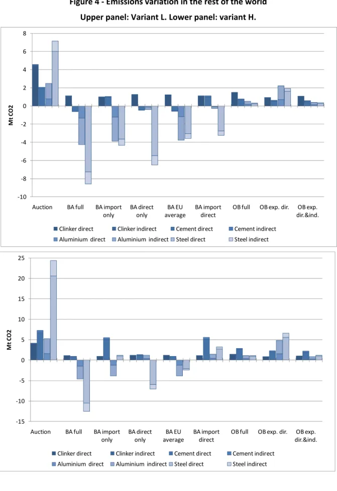
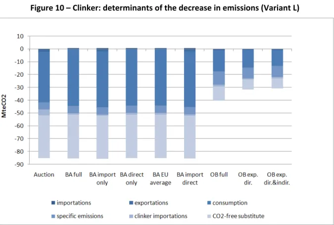
Figure 4 splits up the absolute level of leakage (i.e., the variations in RoW emissions between BAU and climate policy – the numerator of the leakage‐to‐reduction ratio) into sectors. Each bar represents a sector and is split‐up between direct and indirect emissions. The “clinker” bar reports the change in emissions due to the clinker imported from the RoW to the EU. Given that the emissions reduction in the EU is the same whichever the scenario, Figure 4 informs about which scenarios lead to the largest emission decrease worldwide as well.

In the Auction scenario, between 40% (Variant L) and 60% (Variant H) of leakage comes from steel. Leakage from clinker is the same in both variants because the modelling of clinker imports is not based on Armington elasticity but on a logit share function, the parameters of which do not change across variants.

In the steel sector, under Auction, leakage is three times higher in Variant H than in Variant L. The differences are lower for the other climate policies. Also in the steel sector, when a BA is implemented, the inclusion of the export part has a larger impact than the inclusion of the indirect emissions: for instance, in Variant H, BA import only leakage remains positive while it becomes negative with BA direct only. The magnitude of the difference in leakage between BA full and BA EU