Tree-based learning of regulatory network topologies and dynamics with Jump3

topologies and dynamics with Jump3

Vˆan Anh Huynh-Thu and Guido Sanguinetti

Abstract Inference of gene regulatory networks (GRNs) from time series data is a well established field in computational systems biology. Most approaches can be broadly divided in two families: model-based and model-free methods. These two families are highly complementary: model-based methods seek to identify a formal mathematical model of the system. They thus have transparent and interpretable se-mantics, but rely on strong assumptions and are rather computationally intensive. On the other hand, model-free methods have typically good scalability. Since they are not based on any parametric model, they are more flexible that model-based methods, but also less interpretable.

In this chapter, we describe Jump3 [1], a hybrid approach that bridges the gap between model-free and model-based methods. Jump3 uses a formal stochastic dif-ferential equation to model each gene expression, but reconstructs the GRN topol-ogy with a non-parametric method based on decision trees. We briefly review the theoretical and algorithmic foundations of Jump3, and then proceed to provide a step by step tutorial of the associated software usage.

Key words: Hybrid method, decision trees, stochastic differential equations, Gaus-sian processes

Vˆan Anh Huynh-Thu

Department of Electrical Engineering and Computer Science, University of Li`ege, Li`ege, Belgium e-mail: vahuynh@uliege.be

Guido Sanguinetti

School of Informatics, University of Edinburgh, Edinburgh, U.K. e-mail: gsanguin@inf.ed.ac.uk

1 Introduction

Many methods have been proposed for the inference of gene regulatory networks (GRNs) from gene expression time series data. These methods can be broadly di-vided in two families, that we will name here model-based and model-free ap-proaches. Model-based methods first define a formal mathematical model of the system, usually expressed with differential or difference equations. They then recon-struct the GRN topology by learning the parameters of the mathematical model from observed data (including discrete parameters such as network structure). Model-based methods have several advantages: they have a transparent model, which makes them interpretable for human experts, and once learned, this model can be used for predicting the dynamical behaviour of the system in new experimental conditions. However, model-based methods have also several drawbacks: they tend to be com-putationally intensive, and by essence they make very strong assumptions about the system dynamics (e.g. linear dependencies between genes), which are not al-ways justified biologically. Model-free methods on the other hand infer the GRN without defining any prior mathematical model and directly estimate the gene de-pendencies from the data, using more or less sophisticated statistical measures or machine learning-based analyses. These model-free methods are typically highly scalable and can thus be used for the inference of very large networks. Since they are not based on any parametric model, they are much more flexible than model-based methods, but also less interpretable. Moreover, they cannot be used for prediction in a straightforward way.

This chapter presents a hybrid approach to the network inference problem, called Jump3 [1], that bridges the gap between model-based and model-free methods. Jump3 uses a formal stochastic differential equation to model the dynamics of each gene of the network, but reconstructs the GRN topology with a non-parametric method based on decision trees (see Chapter 8 for more details about tree-based GRN inference methods). Jump3 combines the computational efficiency of model-free methods with a biophysically plausible and interpretable model of gene expres-sion; its performance on benchmark tests (described in [1]) is competitive with, or better than, the state-of-the-art, and a fully documented MATLAB implementation is freely available at http://www.montefiore.ulg.ac.be/˜huynh-thu/ Jump3.html.

In the rest of the chapter, we start by briefly reviewing the mathematical and algorithmic bases of Jump3, with the main aim to illustrate how the model-based approach is embedded into a tree learning framework. We then provide a step by step tutorial on the usage of the Jump3 software, using the synthetic data set accom-panying the software as an example.

2 The Jump3 framework

Let us assume that we observe the expression levels of G genes at T time points following some perturbation of the system:

T S= {ˆx1,ˆx2, . . . ,ˆxG}, (1)

where ˆxiis the vector containing the observed expressions of gene giat the T time

points:

ˆxi= ( ˆxi,1, ˆxi,2, . . . , ˆxi,T)> (2)

From this time series data T S, the goal of Jump3 is to learn a weight for each pu-tative regulatory link of the network, with higher weights assigned to links that are true regulatory interactions. Jump3 is a semi-parametric approach: a paramet-ric model is used for modelling the expression of each gene (Section 2.1), but a non-parametric model is used for modelling the regulatory interactions between the genes (Section 2.2).

2.1 The parametric part: modelling gene expression

Jump3 models the dynamics of the expression xi of each gene giusing the on/off

modelof gene expression [2], which uses the following stochastic differential equa-tion (SDE):

dxi= (aiµi(t) + bi− λixi)dt + σsysdw(t) (3)

In this model, the transcription rate of gidepends on the state µiof the promoter of

gi, which can be either active (µi= 1) or inactive (µi= 0). Θi= {ai, bi, λi} is the

set of kinetic parameters. airepresents the efficiency of the promoter in recruiting

polymerase when being in the active state, bi denotes the basal transcription rate,

and λiis the exponential decay constant of xi. The term σsysdw(t) represents a white

noise with variance σsys2 .

Let us assume for the moment that we know the trajectory of the promoter state, i.e. that we know the state µi(t) at any time t. In that case, the SDE (3) is linear and

it can be shown that its solution xi(t) is equivalent to a Gaussian process [3].

Gener-ally speaking, the fact that xi(t) is a Gaussian process means that for any subset of T

time points {t1,t2, . . . ,tT}, the vector (xi(t1), xi(t2), . . . , xi(tT))>follows a

multivari-ate normal distribution with some mean mi∈ RT and covariance Ci ∈ RT×T. In

the specific case of the on/off model, it can be shown that the mean and covariance functions of xi(t) are: mi(t) = xi(0)e−λit+ ai Z t 0 e−λi(t−τ)_µ i(τ)dτ + bi λi (1 − e−λit_{) (4)} Ci(t,t0) = σsys2 2λi (e−λi|t−t0|_{− e}−λi(t+t0)_{) (5)}

Fig. 1 Example of GRN. Circles represent the gene expressions, and squares rep-resent the promoter states. Thick arrows model the pro-moter activations and show the network topology. Figure reproduced from [1], by per-mission of Oxford University Press. x1 x2 x₃ μ1 μ2 μ3

Besides the chosen on/off model, another assumption made by Jump3 is that the gene expression xiis observed at the T time points with i.i.d. Gaussian noise:

ˆ

xi,k = xi(tk) + εi,k, (6)

εi,k ∼N (0,σobs,i,k2 ), k = 1, . . . , T, (7)

where σ_obs,i,k2 is the variance of the observation noise at time point tk for gene gi.

Under this assumption, since both xiand εiare normally distributed, the observed

expression levels ˆxialso follow a multivariate normal distribution:

ˆxi∼N (mi, Ci+ Di), (8)

where Di∈ RT×T is a diagonal matrix with the values σobs,i,k2 along the diagonal.

One can therefore derive the log-likelihood of the observations:

Li= log p(ˆxi) = − T 2log(2π) − 1 2log |Ci+ Di| − 1 2(ˆxi− mi) >_(C i+ Di)−1(ˆxi− mi) (9)

2.2 The non-parametric part: reconstructing the network topology

the assumption that the expressions of giare observed with i.i.d. Gaussian noise, to

compute a likelihood valueLifor any given promoter state trajectory µi.

Now, the second key ingredient of Jump3 is to assume that the promoter state µi

is a function of the expression levels of the genes that are direct regulators of gi(see

Figure 1):

µi(t) = fi(xreg,i(t)) + ξt, ∀t, (10)

where xreg,i(t) is the vector containing the expression levels at time t of the

regula-tors of giand ξtis a random noise with zero mean.

for each target gene gi

Learn jump tree model predicting μi

time ex p res si o n

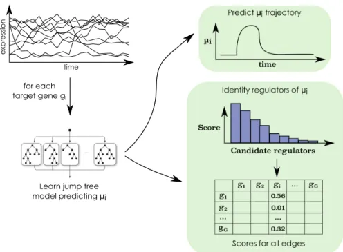
Fig. 2 The Jump3 framework. For each target gene gi, i = 1, . . . , G, a function fiin the form of

an ensemble of jump trees is learned from the time series of expression data. The trajectory of the state of the promoter of gi(µi) is predicted from the jump tree model and an importance score is

computed for each candidate regulator. The score of a candidate regulator gjis used as weight for

the regulatory link directed from gjto gi. Figure reproduced from [1], by permission of Oxford

University Press.

1. To identify the promoter state trajectory µ_i over the time interval [t1,tT] that

maximises the likelihoodLi;

2. To identify the regulators of gi, i.e. the genes whose expression levels are

predic-tive of the promoter state µi.

In principle, these goals could be achieved using a parametric model of promoter ac-tivation, like in [4]; this however necessarily makes strong assumptions on the form of the activation functions, and incurs significant computational overheads. Jump3 instead addresses both problems non-parametrically, by learning the functions fiin

the form of ensembles of decision trees (Figure 2).

2.2.1 Decision trees with a latent output variable

A decision tree is a model that allows to predict the value of an output variable given the values of some input variables, using binary tests of the type “xj< c”, where

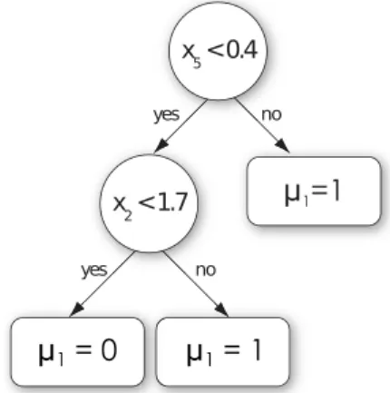
Fig. 3 Example of decision tree. A decision tree is a model that predicts the value of an output variable (here the state µ1of the promoter of

gene g1) from the values of

some input variables (here the expressions levels x2and x5

of candidate regulators g2and

g5respectively). Each interior

node of the tree is a test on the value of one input variable and each terminal node (or leaf) contains a prediction for the output.

are currently one of the state-of-the-art approaches for GRN inference [5, 6]. They have several appealing properties, among which their non-parametric nature (no assumption is made about the function fi) and their scalability (they can be applied

on high-dimensional datasets).

The idea of Jump3 is thus to learn for each target gene gia tree-based model that

predicts the promoter state µi at any time point from the expression levels of the

other genes (or a set of candidate regulators) at the same time point. Traditional tree-based algorithms can however only be used on datasets containing observed values for the input and output variables. In our case, the values of the input variables (i.e. the gene expression levels) are observed at multiple time points, but not the values of the output (i.e. the promoter state µi). We say that µiis a latent variable. Jump3

thus resorts to a new type of decision tree called jump tree, that allows to predict the value of a latent output variable.

Algorithm 1 shows the pseudo-code for growing a jump tree predicting µi. The

idea is to split the data samples (each corresponding to a different time point) into different subsets based on tests on the expression levels of the candidate regulators. For each test, the promoter state µi is assumed to be equal to 0 (resp. 1) at the

time points where the test is true (resp. false). Each new split thus generates a new promoter state trajectory, corresponding to a certain likelihood value. A jump tree is constructed top-down using a greedy algorithm, that iteratively replaces one leaf with a test node in a way to maximise the likelihood. More specifically, the jump tree is initialised as a single leaf, containing all the T observation time points. At each iteration, for each leaf N of the current jump tree and its corresponding set of time points PN, the optimal split of PNis identified, i.e. the test sN= “xj< value” resulting

in the promoter state trajectory that yields the maximum likelihood (lines 5-9 of Algorithm 1). The leaf N∗with the highest maximum likelihood is then replaced

with a test node containing the optimal test sN∗(lines 10-15). The child nodes of this

new test node are two leaves containing respectively the subsets of time points P0

and P1, obtained from PN∗using the test sN∗(this procedure is illustrated in Figure 4).

L1 = -1.39

A

C

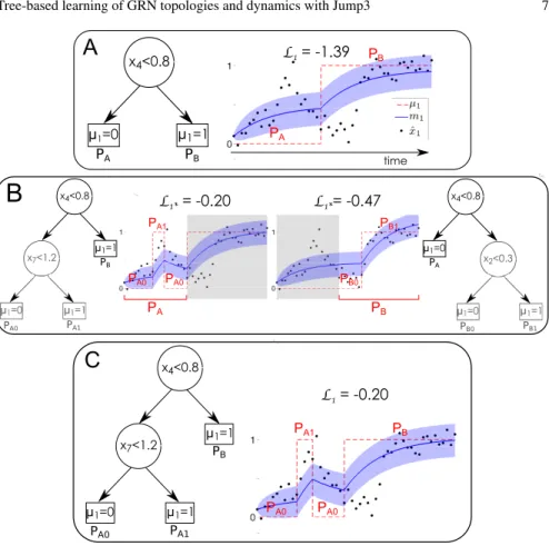
B

Fig. 4 Growing a jump tree predicting the state µ1of the promoter of gene g1. (A) Each iteration

of the jump tree algorithm results in a new tree and a new trajectory µ1(dashed red line) yielding

a likelihoodL1. In this example, the current tree splits the set of observation time points in two

subsets PAand PB, each one corresponding to a leaf of the tree. The plot also shows the posterior

mean m1of the expression of g1(solid blue line), with confidence intervals (shaded area), and the

observed expression levels of g1(black dots). (B) For each leaf of the current tree, the optimal split

of the corresponding set of time points is identified. (C) The leaf for which the optimal split yields the highest likelihood is replaced with a test node. Figure reproduced from [1], by permission of Oxford University Press.

Algorithm 2 shows how to choose a test at a new split node. For each possible test, composed of a candidate regulator gjand a threshold value c (where c is set to

the expression of gjat one time point tk), a candidate promoter state trajectory µj,k

is obtained by setting µ_j,kto 0 (resp. 1) at the time points where the expression of gjis lower (resp. higher) than c (lines 6-12). The test that is selected is then the one

Algorithm 1: buildJumpTree

input : The expressions ˆxiof a target gene giat T time points t1, . . . ,tT, and the expressions

ˆ

XRof R candidate regulators at the same time points

output: A jump tree JT predicting the state µiof the promoter of gi, from the expressions of

the R candidate regulators

1 JT← a leaf containing the set of all the observation time points {t1, . . . ,tT}

2 foreach t between t1and tTdo µi(t) ← 0

3 Li← computeLikelihood(µi,ˆxi)

4 whileLican be increaseddo

5 for each leaf N of JT do

6 PN← getTimePoints(N)

7 (sN, µi,N) ← pickOptimalSplit(ˆxi, ˆXR, PN, µi)

8 Li,N← computeLikelihood(µi,N,ˆxi)

9 end

10 N∗← arg maxNLi,N

11 ifLi,N∗>Lithen

12 µ_i← µ_i,N∗

13 Li←Li,N∗

14 Split PN∗into P0and P1according to sN∗

15 JT← createSplitNode(N∗, sN∗, P0, P1)

16 else

17 return JT

18 Exit while loop

19 end

20 end

2.2.2 Ensemble of decision trees

A single decision tree typically overfits the observed data. This means that the tree model tends to also fit the noise that is contained in the data, leading to bad perfor-mance when predicting unseen data. One solution to reduce overfitting is to grow an ensemble of several trees and to average the predictions of these different trees. A way to obtain different trees is to introduce some randomisation when learning each of the trees. In Jump3, the Extra-Trees procedure is used [7]: at each test node, the best test is selected among a number K of random tests, rather than all the possible tests. Each of the K candidate tests is obtained by randomly selecting one candidate regulator (without replacement) and one threshold value. Each tree of the ensemble will thus have its own prediction of µi(t). This prediction is then averaged over the

different trees, yielding a probability for the promoter state to be active at time t.

2.2.3 Importance measure

Once learned, a single tree or an ensemble of trees can be used to compute a score for each candidate regulator, that measures the importance of that candidate regulator in the tree-based model. The idea is then to use the importance wj,i of candidate

Algorithm 2: pickOptimalSplit

input : The expressions ˆxiof target gene giat T time points t1, . . . ,tT, the expressions ˆXRof

Rcandidate regulators at the same time points, a subset of time points P⊂ {t1, . . . ,tT}, and an initial promoter state trajectory µinit

output: A test in the form “xj< value” and an updated promoter state trajectory

1 for each candidate regulator gj∈ R do

2 for each time point tk∈ P do

3 sj,k← “xj< ˆxj(tk)” // definition of a new test

4 µj,k← µinit

5 for each time point tk0∈ P do

6 if ˆxj(tk0) < ˆxj(tk) then

7 µj,k(tk0) ← 0

8 else

9 µj,k(tk0) ← 1

10 end

11 foreach t between tk0and the next observation time pointdo µj,k(t) ← µj,k(tk0) 12 end 13 Lj,k← computeLikelihood(µj,k,ˆxi) 14 end 15 end 16 ( j∗, k∗) = arg max( j,k)Lj,k

17 return the test sj∗_,k∗_{and the trajectory µ}

j∗,k∗

regulator gjin the model predicting µi(t) as weight for the edge of the GRN that is

directed from gene gjto gene gi.

The importance measure that is used in Jump3 is based on the likelihood gain at each test node N, obtained during the tree learning:

I(N) =Li,N−Li, (11)

whereLi andLi,N are the log-likelihoods respectively obtained before and after

splitting the data samples at node N. For a single tree, the importance score wj,iof

candidate regulator gjis then computed by summing the likelihood gains at all the

tree nodes where there is a test on that regulator:

wj,i= n

∑

k=1

I(N_k)1_Nk(gj), (12)

where n is the number of test nodes in the tree and Nkis the k-th test node.1Nk(gj)

is a function that is equal to one if the test at node Nkuses gj, and zero otherwise.

The candidate regulators that are not used in any test node thus obtain an impor-tance score of zero and those ones that appear in tests close to the root node of the tree typically obtain high scores. When using an ensemble of trees, the importance measure of each candidate regulator is simply averaged over all the different trees.

2.2.4 Regulatory link ranking

Given the definition of the importance score (12), the sum of the scores of all the candidate regulators, for a single tree, is equal to the total likelihood gain yielded by the tree:

∑

j6=i

wj,i=Li−Li,0, (13)

whereLi,0 is the initial log-likelihood obtained with µi(t) = 0, ∀t, and Li is the

final log-likelihood obtained after the tree has been grown. Some regulatory links of the network may therefore receive a high weight only because they are directed towards a gene for which the overall likelihood gain is high. To avoid this bias, the importance scores obtained from each tree are normalised, so that they sum up to one: wj,i← wj,i Li−Li,0 (14) 2.2.5 Kinetic parameters

The on/off model (3) has three kinetic parameters ai, bi and λi. Given a promoter

state trajectory µ_i, the values of aiand biare optimised in order to maximise the

log-likelihoodLi(in line 8 of Algorithm 1, and once the final µitrajectory is obtained

from the tree ensemble). SinceLi is a quadratic function of ai and bi (see

Equa-tions (4) and (9)), these two parameters can be easily optimised using quadratic programming. The value of the decay rate λi is more difficult to optimise, and is

instead directly estimated from the observed expressions of gene gi, by assuming an

exponential decay e−λit _{between the highest and lowest expressions of g}

i.

2.3 Computational complexity

Let us assume for simplicity that each tree contains S test nodes. It can then be shown that the computational complexity of Jump3 is O(GntreesKS2T2), where G

is the number of genes, ntreesis the number of trees per ensemble, K is the number

of randomly chosen candidate regulators at each test node, and T is the number of observation time points. At worst, the complexity of the algorithm is thus quadratic with respect to the number of genes (when K = G − 1) and O(T4) with respect to the number of observations (when S = T − 1, i.e. each tree is fully developed with each leaf corresponding to one time point). Jump3 can thus become computationally intensive when the number of data samples is too high, but remains scalable with respect to the network size.

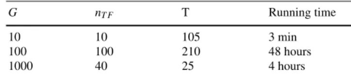
Table 1 gives an idea of the computing times, when using the MATLAB imple-mentation of Jump3. In each case, K was set to the number of candidate regulators

and ntrees was set to 100. These computing times were measured on a 8GB RAM,

1.7 GHz Intel core i7 computer.

Table 1 Running times of Jump3 for varying dataset sizes

G nT F T Running time

10 10 105 3 min

100 100 210 48 hours

1000 40 25 4 hours

G: number of genes, nT F: number of candidate regulators, T : number of observations

2.4 Jump3 performance

The ability of Jump3 to accurately reconstruct network topologies was assessed us-ing several in silico networks (among which the networks of the DREAM4 In Silico Network challenge[6, 8]) as well as one synthetic network (the IRMA network [9]), for which the true topologies are known. For these networks, Jump3 always yields competitive, and often better, performance, compared to other existing, state-of-the-art network inference methods.

Jump3 was also applied to a real gene expression dataset related to murine macrophages [10], in order to retrieve regulatory interactions that are involved in the immune response. The predicted network (composed of the 500 top-ranked in-teractions) is highly modular, with a few transcription factors acting as hub nodes, each one regulating a large number of target genes. These hub transcription fac-tors were found to be biologically relevant, comprising some interferon genes, one gene known to be associated with cytomegalovirus infection and several cancer-associated genes.

The interested reader can find additional details and all the results of these exper-iments in the original paper [1].

3 The Jump3 code

Jump3 was implemented and tested in MATLAB. A fully documented implementa-tion of Jump3 is available at

http://www.montefiore.ulg.ac.be/˜huynh-thu/Jump3.html In this section, we provide a tutorial showing how to run the code using the synthetic example data provided with the implementation; to run it on a different data set, one simply needs to provide a new data file.

3.1 Run Jump3

First of all, add the directory ’jump3 code’ into MATLAB’s path:

path(path,'path_to_the_directory/jump3_code')

A MATLAB file ’exampleData.mat’ is provided for this tutorial.

load exampleData.mat who

## Your variables are: ##

## data genes obsTimes

• data contains the (simulated) expression data of 10 genes from 5 times se-ries. This is a toy dataset that was obtained by simulating the on/off model in Equation (3). Noisy observations at several time points were obtained from the simulated expression time series by adding i.i.d. Gaussian noise.

• obsTimes contains the observation time points for each time series of data. • genes contains the names of the genes.

3.1.1 Noise parameters

Jump3 has two noise parameters. These parameters must be put in a structure array (that we will name here noiseVar) with two fields that must be named sysNoise and obsNoise.

• noiseVar.sysNoise is the variance of the intrinsic noise (σsys2 ); one single

value.

• noiseVar.obsNoise is the variance of the observation noise (σ_obs,i,k2 ); one value for each data value.

The optimal values of the noise parameters are difficult to identify (in most cases, trying to optimise these parameters would result in local optima). Some heuristic should thus be used to set the values of these parameters. For example, a dynamic noise can be used for the observation noise, assuming that the observation noise is higher for higher expression values:

noiseVar.obsNoise = cell(1,length(data));

for k=1:length(data)

noiseVar.obsNoise{k} = (data{k}/10).ˆ2;

% Replace zero values with a small number % to avoid numerical errors

noiseVar.obsNoise{k}(noiseVar.obsNoise{k}==0) = 1e-6; end

The intrinsic noise can be assumed to be much smaller than the observation noise:

noiseVar.sysNoise = 1e-4;

3.1.2 Run Jump3 with its default parameters

[w,exprMean,exprVar,promState,kinParams,kinParamsVar,trees] = ...

jump3(data,obsTimes,noiseVar); (This should take a few minutes.)

By default, all the genes are candidate regulators, the parameter K of the Extra-Trees (i.e. the number of randomly chosen candidate regulators at each test node) is set to the total number of candidate regulators and the number ntreesof trees per

ensemble is set to 100.

The algorithm outputs the following:

• w: weights of the regulatory links. w(i,j) is the weight of the link directed from gene gjto gene gi.

• exprMean: posterior mean mi(t) of the expression of each gene giin each time

series.

• exprVar: posterior variance ci(t,t) of the expression of each gene gi.

• promState: posterior state µi(t) of the promoter of each gene giin each time

series.

• kinParams: (optimised) values of the kinetic parameters ai, bi, and λifor each

gene gi.

• kinParamsVar: variances of the kinetic parameters aiand bi.

• trees: ensemble of jump trees predicting the promoter state of each gene gi.

3.1.3 Restrict the candidate regulators to a subset of genes

To guide the network inference, the candidate regulators can be restricted to a subset of genes (for example the genes that are known to be transcription factors).

% Indices of the genes that are used as candidate regulators

w2 = jump3(data,obsTimes,noiseVar,tfidx);

In w2, the links that are directed from genes that are not candidate regulators have a score equal to 0.

3.1.4 Change the settings of the Extra-Trees

It is possible to set the values of the two parameters of the Extra-Trees algorithm (K and ntrees).

% Extra-Trees parameters

K = 3; ntrees = 50;

% Run the method with these settings

w3 = jump3(data,obsTimes,noiseVar,1:10,K,ntrees);

3.1.5 Obtain more information

Additional information about the function jump3() can be found by typing this command:

help jump3

3.2 Write the predictions

3.2.1 Get the predicted ranking of all the regulatory links

Given the weight matrix w returned by the function jump3(), the ranking of reg-ulatory links (where the links are ordered by decreasing order of weight) can be retrieved with the function getLinkList().

getLinkList(w)

The output will look like this: ## G8 G6 0.886894 ## G3 G7 0.841794 ## G9 G10 0.831725 ## G1 G5 0.782503

## G1 G2 0.715546 ## G7 G3 0.512323 ## ...

Each line corresponds to a regulatory link. The first column shows the regulator, the second column shows the target gene, and the last column indicates the weight of the link.

If the gene names are not provided, the i-th gene is named “Gi”.

Note that the ranking that is obtained will be slightly different from one run to another. This is due to the intrinsic randomness of the Extra-Trees. The variance of the ranking can be decreased by increasing the number of trees per ensemble.

3.2.2 Show only the links that are directed from the candidate regulators

The set of candidate regulators can be specified, to avoid displaying the links that are directed from genes that are not candidate regulators and have hence a score of zero.

getLinkList(w2,tfidx)

3.2.3 Show the top links only

The user can specify the number of top-ranked links to be displayed. For example, to show only the first five links:

ntop = 5;

getLinkList(w2,tfidx,{},ntop)

3.2.4 Show the names of the genes

The ranking can be shown with the actual gene names, rather than the default names:

getLinkList(w2,tfidx,genes,5) ## FAM47B RXRA 0.983707 ## ZNF618 RFC2 0.839112 ## GPX4 CYB5R4 0.808789 ## CYB5R4 NPY2R 0.674845 ## CYB5R4 GPX4 0.673964

3.2.5 Write the predicted links in a file

Instead of displaying the edge ranking in the MATLAB console, the user can choose to write it in a file (named here “ranking.txt”):

getLinkList(w,1:10,genes,0,'ranking.txt')

3.2.6 Obtain more information

Additional information about the function getLinkList() can be found by typ-ing this command:

help getLinkList

3.3 Plot the modelling results

The posterior mean expression of one gene in one time series, as well as the pre-dicted promoter state trajectory, can be plotted with the function plotPosteriors().

% Plot the results for the fifth gene in the first time series

TSidx = 1; geneidx = 5;

plotPosteriors(data,obsTimes,exprMean,exprVar,promState,...

TSidx,geneidx)

Figure 5 shows an example of plot returned by this command.

3.3.1 Obtain more information

Additional information about the function plotPosteriors() can be found by typing this command:

Fig. 5 The top plot shows the posterior mean expression of the target gene (solid red line) with the confidence intervals (shaded red area), as well as the observed expression of the gene (black dots). The bottom plot shows the predicted state of the promoter of the gene.

4 Conclusion

Reconstructing GRNs from time series data is a central task in systems biology, and several methods are currently available. In this chapter, we reviewed a recent method, Jump3, which combines some of the advantages of model-based methods with the speed and flexibility of non-parametric, tree-based learning methods. The focus of this chapter is twofold: we first provide a brief introduction to the mathe-matical aspects of the Jump3 framework, focussing on the practical aspects of ex-tracting relevant statistics from the algorithm’s output. We then provide a step by step tutorial on how to use the MATLAB implementation of Jump3, freely available at http://www.montefiore.ulg.ac.be/˜huynh-thu/Jump3.html. We hope that this chapter will enhance the usability of Jump3, reinforcing its status as a useful tool within the GRN inference toolkit.

Acknowledgements VAHT is a Post-doctoral Fellow of the F.R.S.-FNRS. GS acknowledges sup-port from the European Research Council under grant MLCS 306999.

References

[1] Huynh-Thu VA, Sanguinetti G (2015) Combining tree-based and dynami-cal systems for the inference of gene regulatory networks. Bioinformatics 31(10):1614–1622

[2] Ptashne M, Gann A (2002) Genes and Signals. Cold Harbor Spring Laboratory Press, New York

[3] Gardiner CW (1996) Handbook of Stochastic Methods. Springer, Berlin [4] Ocone A, Millar AJ, Sanguinetti G (2013) Hybrid regulatory models: a

sta-tistically tractable approach to model regulatory network dynamics. Bioinfor-matics 29(7):910–916

[5] Huynh-Thu VA, Irrthum A, Wehenkel L, Geurts P (2010) Inferring regula-tory networks from expression data using tree-based methods. PLoS ONE 5(9):e12,776

[6] Marbach D, Costello JC, K¨uffner R, Vega N, Prill RJ, Camacho DM, Al-lison KR, the DREAM5 Consortium, Kellis M, Collins JJ, Stolovitzky G (2012) Wisdom of crowds for robust gene network inference. Nature Meth-ods 9(8):796–804

[7] Geurts P, Ernst D, Wehenkel L (2006) Extremely randomized trees. Machine Learning 36(1):3–42

[8] Prill RJ, Marbach D, Saez-Rodriguez J, Sorger PK, Alexopoulos LG, Xue X, Clarke ND, Altan-Bonnet G, Stolovitzky G (2010) Towards a rigorous as-sessment of systems biology models: The DREAM3 challenges. PLoS ONE 5(2):e9202

[9] Cantone I, Marucci L, Iorio F, Ricci MA, Belcastro V, Bansal M, Santini S, di Bernardo M, di Bernardo D, Cosma MP (2009) A yeast synthetic network for in vivo assessment of reverse-engineering and modeling approaches. Cell 137(1):172–181

[10] Blanc M, Hsieh WY, Robertson KA, Watterson S, Shui G, Lacaze P, Khon-doker M, Dickinson P, Sing G, Rodr´ıguez-Mart´ın S, Phelan P, Forster T, Strobl B, M¨uller M, Riemersma R, Osborne T, Wenk MR, Angulo A, Ghazal P (2011) Host defense against viral infection involves interferon mediated down-regulation of sterol biosynthesis. PLoS Biology 9(3):e1000,598