L. Prevost, S. Marinai, and F. Schwenker (Eds.): ANNPR 2008, LNAI 5064, pp. 280–291, 2008. © Springer-Verlag Berlin Heidelberg 2008
Descriptors in Dimensionality Reduction Context: An
Overview Exploration
Ludovic Journaux1, Marie-France Destain1, Johel Miteran2, Alexis Piron1, and Frederic Cointault3
1
Unité de Mécanique et Construction, Faculté Universitaire des Sciences Agronomiques de Gembloux, Passage des Déportés 2, B-5030 Gembloux, Belgique
2
Lab. Le2i, Université de Bourgogne, BP 47870, 21078 Dijon Cedex, France
3
ENESAD UP GAP, 26 Bd Dr Petitjean BP 87999, 21079 Dijon Cedex, France [email protected]
Abstract. In the context of texture classification, this article explores the capacity and the performance of some combinations of feature extraction, linear and nonlinear dimensionality reduction techniques and several kinds of classification methods. The performances are evaluated and compared in term of classification error. In order to test our texture classification protocol, the experiment carried out images from two different sources, the well known Brodatz database and our leaf texture images database.
Keywords: Texture classification, Motion Descriptors, Dimensionality reduction.
1 Introduction
For natural images the texture is a fundamental characteristic which plays an important role in pattern recognition and computer vision. Thus, texture analysis is an essential step for any image processing applications such as medical and biological imaging, industrial control, document segmentation, remote sensing of earth resources. A successful classification or segmentation requires an efficient feature extraction methodology but the major difficulty is that textures in the real world are often not uniform, due to changes in orientation, scale, illumination conditions, or other visual appearance. To overcome these problems, numerous approaches are proposed in the literature, often based on the computation of invariants followed by a classification method as in [1]. In the case of a large size texture image, these invariants texture features often lead to very high-dimensional data, the dimension of the data being in the hundreds or thousands. Unfortunately, in a classification context these kinds of high-dimensional datasets are difficult to handle and tend to suffer from the problem of the “curse of dimensionality”, well known as “Hughes phenomenon” [2], which cause inaccurate classification. One possible solution to improve the classification performance is to use Dimensionality Reduction (DR) techniques in order to transform high-dimensional data into a meaningful representation of reduced
dimensionality. Numerous studies have aimed at comparing DR algorithms, usually using synthetic data [3 , 4] but less for natural tasks as in [5] or [6].
In this paper, considering one family of invariants called Motion descriptors (MD) or Generalized Fourier Descriptors (GFD) [7] which provide well-proven robust features in complex areas of pattern recognition (faces, objects, forms) [8], we propose to compare in 6 classification methods context, the high-dimensional original features datasets extracted from two different textures databases to reduced textures features dataset obtained by 11 DR methods. This paper is organized as follows : section 2 presents the textured images databases, review the definition of invariants features used for classification methods which are also quickly described. In section 3 we propose a review of Dimensionality Reduction techniques and the section 4 presents the results allowing to compare the performances of some combinations of feature extraction, dimensionality reduction and classification. The performances are evaluated and compared in term of classification error.
2 Materials and Methods
2.1 Textures Images Databases
In order to test our texture classification protocol, the experiment carried out images from two different sources:
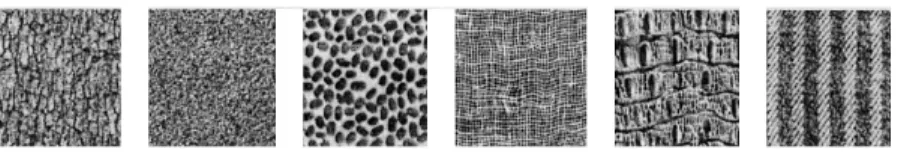
The well known Brodatz textures dataset [9] adapted from the Machine Vision Group of Oulun University and first used by Valkealahti [10]. The dataset is composed of 32 different textures (Fig. 1). The original images are grey levels images with a 256 256× pixels resolution. Each image has been cropped into 16 disjoint 64x64 samples. In order to evaluate scale and rotation invariance, three additional samples were generated per original sample (90° degrees rotation, 64 64× scaling, combinations of rotation and scaling). Finally, the set contains almost 2048 images, 64 samples per texture.
Fig. 1. The 32 Brodatz textures used in the experiments
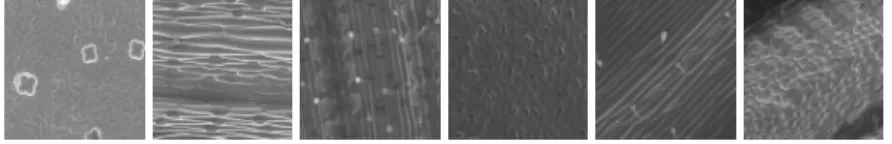
The second textures images used in this study have been provided by the Matters and Materials laboratory at the “Free University of Brussels” for agronomic application. They are grey levels images acquired with a scanning electron microscope (SEM) and representing different kinds of leaf surfaces coming from six leaf plant species (Fig. 2). Thus, the image database contains 6 classes of leaf textures images. For each class 150 to 200 images have been acquired. Each image consists of a 100 µm scale image, with a resolution of 512
×
512 pixels adapting the scale to our biological application (1242 textures images in six classes).Fig. 2. The six classes of leaf texture images
2.2 Texture Characterisation Using Generalized Fourier Descriptors (GFD)
The GFD are defined as follows. Let f be a square summable function on the plane, and ˆf its Fourier transform:
(
)
2 ˆ( ) ( )exp . f ξ =∫
f x −j x dxξ \ (1) If( )
λ θ are polar coordinates of the point ξ , we shall denote again , f λ θ the ˆ ,( )
Fourier transform of f at the point( )
λ θ . Gauthier et al. [7] defined the mapping ,f D from \ into + \ by +
( )
2 2 0 ˆ = ( , ) . f D f d π λ∫
λ θ θ (2)So, D is the feature vector (the GFD) which describes each texture image and will f
be used as an input of the supervised classification method and be reduced by DR methods.
Motion descriptors, calculated according to equation (2), have several properties useful for object recognition : they are translation, rotation and reflexion-invariant [7, 8].
2.3 Classification Methods
Classification is a central problem of pattern recognition [11] and many approaches to solve it have been proposed such as connectionist approach [12] or metrics based methods, k-nearest neighbours (k-nn) and kernel-based methods like Support Vector Machines (SVM) [13], to name the most common. In our experiments, we want to evaluate the average performance of the dimensionality reduction methods and one basic feature selection method applied on the GFD features. In this context, we have chosen and evaluated six efficient classification approaches coming from four classification families: The boosting (adaboost) family [14] using three weak classifiers, (Hyperplan, Hyperinterval and Hyperrectangle), the Hyperrectangle (Polytope) method [15], the Support Vector Machine (SVM) method [13, 16] and the connectionist family with a Multilayers perceptron (MLP) [17]. We have excluded the majority of neural networks methods due to the high variability of textures from natural images; Variability which included an infinite number of samples required for the learning step (Kind of leaves, growth stage, pedo-climatic conditions, roughness, hydration state,…). In order to validate the classification performance and estimate
the average error rate for each classification method, we performed 20 iterative experiments with a 10-fold cross validation procedure.
3 Dimensionality Reduction Methods
The GFD provide features that are of great potential in pattern recognition as it was shown by Smach et al. in [8]. Unfortunately, these high dimensional datasets are however difficult to handle, the information is often redundant and highly correlated with one another. Moreover, data are also typically large, and the computational cost of elaborate data processing tasks may be prohibitive. Thus, to improve the classification performance it is well interesting to use Dimensionality Reduction (DR) techniques in order to transform high-dimensional data into a meaningful representation of reduced dimensionality. At this time of our work, we selected a dozen of DR methods. However, it is important to note that works employing recent approaches as it could be find in [18] are being finalized (another distance, topology or angle preservation methods like Kernel Discriminant Analysis, Generative Topographic Mapping, Isotop, Conformal Eigenmaps,…).
3.1 Estimating Intrinsic Dimensionality
Let ( ,...,1 )
T n =
X x x be the n×m data matrix. The number n represents the number of images examples contained in each texture dataset, and m the dimension of the vector
i
x , which his the vector corresponding to the discrete computing of the D (from eq. f
(2)). We have in our case n=2048 and m=32 for Brodatz textures database and n=1034 and m=254 for plants leaf textures database. This dataset represent respectively 32 and 6 classes of textures surfaces.
Ideally, the reduced representation has a dimensionality that corresponds to the intrinsic dimensionality of the data. One of our working hypotheses is that, though data points (all texture image) are points in \ , there exists a p-dimensional manifold m
1
( ,..., n)T
= y y
M that can satisfyingly approximate the space spanned by the data points. The meaning of “satisfyingly” depends on the dimensionality reduction technique that is used. The so-called intrinsic dimension (ID) of X in \ is the m
lowest possible value of p (p<m) for which the approximation of X by M is
reasonable. In order to estimate the ID of our two datasets, we used a geometric approach that estimates the equivalent notion of fractal dimension [19]. Using this method, we estimated and fixed the intrinsic dimensionality of our two datasets as being p=5.
3.2 Review of DR Methods
DR methods can be classified according to three characteristics:
- Linearity : DR can be Linear or nonlinear. This describes the type of transformation applied to the data matrix, mapping it from \ to m \ . p
- Scale analysis : DR can be Local or global. This reflects the kind of properties the transformation does preserve. In most nonlinear methods, there is a compromise to be made between the preservation of local topological relationships between data points, or of the global structure of X.
- Metric : Euclidean or geodesic. This defines the distance function used to estimate whether two data points are close to each other in \ , and should con-m
sequently remain close in \ , after the DR transformation. p
In this context, we retained 11 methods based on these various criteria, 3 are linear methods and 8 are nonlinear. In order to complete this review of dimensionality reduction methods, we opposed them to one classical feature selection method. This comparison will show which approaches are the most relevant.
3.2.1 Linear Methods
3.2.1.1 Principal Components Analysis. Principal Components Analysis (PCA, [11]) is the best known DR method. PCA finds a linear transformation for keeping the subspace that has largest variance. PCA aims at solving the following problem: given p<m, find an orthonormal basis <u u1, 2,...,up >that minimizes the so-called
reconstruction error: 2 1 (X, ) , n PCA i i i J p = =
∑
x −y (3)It can be shown that JPCA is minimized for the
u
ibeing the eigenvectors of the covariance matrix of X . In practice, it is implemented using singular value decomposition. PCA is linear, global and Euclidean technique.3.2.1.2 Second-Order Blind Identification. Second Order Blind Identification (SOBI) [20] relies only on stationary second-order statistics that are based on a joint diagonalization of a set of covariance matrices. The set X is assimilated to a set of signals ( )X ti and the p features of the destination space we are searching are assimilated to a fixed number of original sources ( )s ti . Each X ti( ) is assumed to be an instantaneous linear mixture of n unknown components (sources) ( )s ti , via the unknown mixing matrix A .
( ) ( )
X t =As t (5)
This algorithm can be described by the following steps (more details on SOBI algorithm can be found in [20]) : (1) Estimate the sample covariance matrix Rx(0)and compute the whitening matrix W with Rx(0)=E X t X t( ( ). *( )). (2) Estimate the covariance matrices Rz( )τ of the whitened process z t( ) for fixed lag times τ . (3) Jointly diagonalize the set {Rz( ) /τj j=1,..., }k , by minimizing the criterion
2 , 1,..., 1,..., ( , ) ( ( t ) i j k n i j n J M V V M V = ≠ = =
∑ ∑
(6)where M is a set of matrices in the form Mk =VD Vk , where V is a unitary matrix, and k
D is a diagonal matrix. (4) Determinate an estimation Aˆof the mixing matrix A such as A Wˆ= −1. (5) Determinate the source matrix and then extracting the p components. SOBI is a linear, global and Euclidean method.
3.2.1.3 Projection Pursuit (PP). This projection method [21] is based on the optimization of the gradient descent. Our algorithm uses the Fast-ICA procedure [22] that allows estimating the new components one by one by deflation. The symmetric decorrelation of the vectors at each iteration was replaced by a Gram-Schmidt orthogonalization procedure. When p components
w
1,...,
w
p have been estimated, thefix point algorithm determines wp+1. After each iteration, the projections
1 ( 1,..., )
T
p j j
w +w w j= p of the p precedent estimated vectors are subtracted from wp+1.
Then, wp+1 is re-normalized: 1 1 1 1 1 1 1 p T p p p j p j j T p p w w w w w w w w + + + = + + + = −
∑
= (7)The algorithm stops when p components have been estimated. Projection Pursuit is linear, global and Euclidean.
3.2.2 Nonlinear Methods : Global Approaches
3.2.2.1 Sammon's Mapping (Sammon). Sammon's mapping is a projection method that tries to preserve the topology of the set of data (neighbourhood) in preserving distances between points [23]. To evaluate the preservation of the neighbourhood topology, we use the following stress function
2 , , , 1 , , , 1 ( ) 1 n m p i j i j sam n m m i j i j i j i j d d J d d = = ⎛ − ⎞ = ⎜⎜ ⎟⎟ ⎝
∑
⎠∑
(8) Where m, i j d and ,p i jd are the distances between points ithand jthpoints, in \ and m \ . p
This function, minimized by a gradient descent, allows adapting the distances in the projection space at best as distances in the initial space. Sammon’s mapping is a nonlinear, global, and Euclidean method.
3.2.2.2 Isometric Feature Mapping (Isomap). Isometric Feature Mapping (Isomap) [24] estimates the geodesic distance along the manifold using the shortest path in the nearest neighbours’ graph. It then looks for a low-dimensional representation that approximates those geodesic distances in the least square sense (which amounts to MDS). It consists of three steps: (1) Build D (X) , the all-pairs distance matrix. (2) m Build a graph from X (k nearest neighbours). For a given point xi in
m
\ , a neighbour is either one of the K nearest data points from xi or one for which m
ij
d <ε. Build the all-pairs geodesic distance matrix Δm(X), using Dijkstra’s all-pairs shortest path
algorithm. (3) Use classical MDS to find the transformation from \ to m \ that p minimizes 2 , ( , ) ( ) n m p ISOMAP ij ij i j J X p =
∑
δ δ− (9)Isomap is nonlinear, global and geodesic.
3.2.2.3 Kernel Methods (K-PCA, K-Isomap). Recently, several well-known algo-rithms for dimensionality reduction of manifolds have been developed in a new way, taking the kernel machine viewpoint [25, 26]. We retain here the two most known : the kernel-PCA (K-PCA) [27] and the kernel Isomap (K-Isomap) [28]. The non-linearity is introduced via a mapping of the data from the input space \ to a feature m
space F . Projection methods (PCA or Isomap) are then performed in this new feature space. This feature space is expressed by a kernel K in terms of a Mercer Kernel function [29]. More details on K-PCA and K-Isomap algorithm can be found respectively in [27] and [28]. These methods are nonlinear and global, K-PCA is Euclidean and K-Isomap is geodesic.
3.2.3 Nonlinear Methods: Local Approaches
3.2.3.1 Local Linear Embedding (LLE). The LLE algorithm [30] estimates the local coordinates of each data point in the basis of its nearest neighbours, then looks for a low-dimensional coordinate system that has about the same expansion. The 3 steps are: (1) Find the neighbourhood graph (see steps 1 and 2 of Isomap). (2) Compute the weights Wij that best reconstruct xi from its neighbours, thus minimizing the reconstruction error, xi−x , where ˆˆi i ij j i
j W
=
∑
≈x x x . (3) Compute vectors y in i
p
\ reconstructed by the weights W . Solve for all ij y simultaneously. i
i ij j
j W
≈
∑
y y (10)
LLE is nonlinear, local and Euclidean. It finds the local affine structure of the data manifold, and identifies the manifold by joining the affine patches.
3.2.3.2 Laplacian Eigenmaps (Laplacian). Similar to LLE, Laplacian Eigenmaps find a low-dimensional data representation by preserving local properties of the manifold [31]. The three steps of the algorithm are the following: (1) Build the non-oriented symmetric neighbourhood graph. (2) Associate a positive weight
ij
W to each link of the graph. These weights can be constant (Wij =1 /k), or
exponentially decreasing (
(
2 2)
exp /
ij i j
W = − x −x σ ). (3) Obtain the final coordinates i
y of the points in \p
(
2)
/ LE ij i j ii jj ij J =∑
W y −y D D (11) where D is the diagonal matrix Dii=∑
jWij . The minimum of the cost function is found with the eigenvectors of the Laplacian matrix:1 1
2 2
L= −I D− −WD− . LE is a nonlinear, local, Euclidean method.
3.2.3.3 Curvilinear Components Analysis (CCA). CCA is an evolution of the nonlinear Multidimensional Scaling (MDS) and Sammon’s mapping algorithms [32]. Instead of the optimization of a reconstruction error, CCA and the related Curvilinear Distance Analysis (CDA) aim at preserving of the so-called distance matrix while projecting data onto a lower dimensional manifold.
Let (X)Dm be the
2 2
n ×n matrix of distances between pairs of points in X (X) ( m),
m ij
D = d where m
ij i j
d = x −x (12)
After DR transformation to
\
p, we also have (X) ( p),p ij
D = d where p
ij i j
d = y −y (13)
As with PCA, the yiare the transformed approximations of the xi. CCA tries to find the best suitable transformation, minimizing
2 , 1 (X, ) ( ) ( ), n m p p CCA ij ij ij i j J p d d F d = =
∑
− (14)Where
F
is a decreasing, positive function. It acts as a weighting function, giving more importance to the preservation of small distances. In practice, JCCA is minimized using stochastic gradient descent and vector quantization to limit the optimization to a reduced set of representative points. CCA is nonlinear, local and Euclidean.CDA is a refinement of CCA [4], minimizing
2 , 1 (X, ) ( ) ( ), n m p p CDA ij ij ij i j J p δ d F d = =
∑
− (15)Where
δ
ijmmeasures the geodesic distance between xiandxj, approximated by the shortest path distance along a neighbourhood graph. CDA is nonlinear, local and geodesic.3.2.4 Feature Selection Method
Parameter selection with an exhaustive search is impractical due to the large amount of possible feature subsets. To select the 5 best parameters, we use sequential forward selection (SFS) [33]. The criteria function is the average correct classification rate over all classes, obtained by quadratic discriminant analysis (QDA) on all
observations. The QDA approach was chosen because it is not dependant on parameters other than the observations and that the goal is not to compute the optimal classification rate but a measure of the feature subsets efficiencies. At the end of the process, the 5 best features have been selected.
4 Results
In order to compare the classification performance and estimate the average error rate for each classification method, we performed 20 iterative experiments with a 10-fold cross validation procedure. In the case of SVM, we used the gaussian kernel, for which we tuned the determined the optimum value of :
2 ( , ) K e σ ⎛ − ⎞ ⎜− ⎟ ⎜ ⎟ ⎝ ⎠ = x y x y (16)
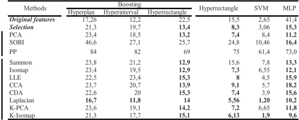
Table 1. Classification results on the Brodatz dataset (% error rate)
Hyperplan Hyperinterval Hyperrectangle
17,26 12,2 22,5 15,5 2,65 41,4 Selection 21,3 19,7 13,4 8,3 3,06 15,3 PCA 23,4 18,5 13,2 7,4 8,4 11,2 SOBI 46,6 27,1 25,7 24,8 10,46 16,4 PP 84 82 69 75 61,4 73,0 Sammon 23,8 21,2 12,9 15,6 7,8 13,3 Isomap 23,4 19,5 12,9 7,3 6,55 12,1 LLE 22,5 23,4 15,3 8 4,5 15,9 CCA 23,7 20,7 13,9 9,1 5,7 18,2 CDA 22,6 20 15,3 7,4 3,9 15,6 Laplacian 16,7 11,8 14 5,56 1,20 10,2 K-PCA 23,6 19,1 14,2 7,2 6,65 11,8 K-Isomap 21,3 17,7 15,1 6,13 1,9 9,6 no nline ar SVM MLP Original features line ar
Methods Boosting Hyperrectangle
In the case of Brodatz texture dataset (Table 1), regarding to the classification error using the original feature space, the best result are obtained using SVM (e=2.65%). In this case, the backpropagation algorithm of the MLP seems to converge to a local minimum and not to the global one. The use of a second order optimization method, such as BFGS or Levenberg-Marquart method [34] could overcome this problem. All the other methods give poorer results (from 12.2% to 22.5%). Their performances are generally improved by DR: the optimum error is obtained combining Laplacian Eigenmaps and SVM (e=1.2%, i.e. the error is divided by a factor 2). The K-Isomap combination with SVM gives some similar results. One can note that the use of kernel in DR methods generally improve performances compared to original ones (Isomap vs K-Isomap, PCA vs K-PCA). In the family of fast decision methods, the best result is obtained using Hyperrectangle also combined with Laplacian Eigenmaps.
These results are generally confirmed by the experiments performed using the plants Leaf dataset (Table 2), although the original dimensional space is significantly higher than in the previous case (254 vs 32) and the number of classes is lower (6 vs 32). In this case, the gain factor is 1.18 (comparing SVM using original feature space, and SVM combined with Laplacian Eigenmaps).
Table 2. Classification results on the Plants leaf dataset (% error rate)
Hyperplan Hyperinterval Hyperrectangle
6,52 3,3 16,87 27,61 1,47 35,7 Selection 18,19 14,97 3,7 10,5 5,71 9,7 PCA 7,64 3,94 8,62 9,66 2,35 11,9 SOBI 15,29 4,99 9,56 13,2 4,8 15,8 PP 87,2 85,58 87,45 84,54 82 81,2 Sammon 26,9 25,84 10,89 10,1 5,48 13 Isomap 7,2 5,12 4,25 7,8 2,28 11,2 LLE 22,86 17,87 7,81 8,29 1,96 14,1 CCA 31,07 17,47 5,23 9,98 2,89 16,2 CDA 34,13 7,6 4,83 9,75 1,92 15,4 Laplacian 5,2 2,5 10,38 8,1 1,25 7,8 K-PCA 7,05 13,2 11,75 11,51 1,86 13,9 K-Isomap 6,8 3,9 11,43 6,3 1,31 10,2 no nlin ea r SVM MLP Original features li nea r
Methods Boosting Hyperrectangle
In order to classify the DR methods, we computed the average rank of each method for both datasets (Table 3). Laplacian Eigenmaps and K-Isomap are the best ranked, but the standard PCA (linear) is still a good compromise between computation time and performances.
Table 3. Average rank mean for each classification results for the two dataset
Hyperplan Hyperinterval Hyperrectangle
Laplacian 1 1 7 2 1 1,5 2,25 K-Isomap 3 3 9 1,5 2 2 3,42 Isomap 6 6 1,5 3 7,5 4,5 4,75 PCA 7 4 4,5 5,5 9,5 4 5,75 Selection 6 8 2,5 8,5 8 4,5 6,25 K-PCA 6,5 6,5 9 6,5 6,5 5,5 6,75 Original data 2 2 11,5 11 3 12 6,92 CDA 9 7,5 6 5,5 5 8,5 6,92 LLE 7 11 7,5 5,5 6 8,5 7,58 CCA 10,5 9,5 4,5 8 8 11 8,58 Sammon 10,5 11 5,5 9,5 10,5 6 8,83 SOBI 9,5 8,5 9,5 11,5 11 10 10,00 PP 13 13 13 13 13 13 13,00 MLP rank means Methods Boosting Hyperrectangle SVM
Moreover, it is interesting to note that DR methods allow to minimize the number of support vectors needed for the decision function of SVM (Table 4). For Laplacian Eigenmaps, the gain is 29% in the case of Brodatz dataset and 47% in the case of Plants leaf dataset. Since the computation time of the SVM decision function depends linearly of this number, the process is accelerated. This is particularly true using PCA, since it is not always necessary to update the PCA transformation during the classification step.
Table 4. Number of support vectors needed for the decision function of SVM
Dataset Original
data Selection CCA SOBI PCA K-PCA CDA LLE Lapl K-iso Iso Sam PP Brodatz 1545 1120 1006 1025 1035 1050 1059 1078 1095 1155 1163 1189 1467 Plants leaf 504 209 363 172 232 332 419 291 267 296 328 272 1090
5 Conclusion
In this paper we proposed a comparison of DR methods combined with several classification methods, in the context of texture classification of natural images using GFD. We used the powerful Generalized Fourier Descriptors which have interesting properties such as translation, rotation and reflexion invariants.
In any case, the SVM classifier outperforms all other classification methods using the original feature space. However, we experimentally demonstrated that some DR methods still improve final classification performances, and we proposed a rank classification of these methods. The best DR methods are the Laplacian Eigenmaps and K-Isomap, even if the standard PCA is still a good compromise between computation time and performances. In any case, the use of DR methods allows to minimize the number of support vectors, thus optimizing the computational cost of the final decision step.
In our future work, we will apply this comparison review to multispectral textures images for which the original dimensional space is higher and for which the correlation between spectral bands are often very important.
References
1. Arivazhagan, S., Ganesan, L., Priyal, S.P.: Texture classification using Gabor wavelets based rotation invariant features. Pattern Recognition Letters 27, 1976–1982 (2006) 2. Hughes, G.F.: On the mean accuracy of statistical pattern recognizers. IEEE Transactions
on Information Theory 14, 55–63 (1968)
3. Aldo Lee, J., Archambeau, C., Verleysen, M.: Locally Linear Embedding versus Isotop. In: ESANN 2003 proceedings, Bruges (Belgium), pp. 527–534 (2003)
4. Aldo Lee, J., Lendasse, A., Verleysen, M.: Nonlinear projection with curvilinear distances: Isomap versus curvilinear distance analysis. Neurocomputing 57, 49–76 (2004)
5. Journaux, L., Foucherot, I., Gouton, P.: Reduction of the number of spectral bands in Landsat images: a comparison of linear and nonlinear methods. Optical Engineering 45, 67002 (2006)
6. Niskanen, M., Silven, O.: Comparison of dimensionality reduction methods for wood surface inspection. In: QCAV 2003 proceedings, Gatlinburg, Tennessee, USA, pp. 178– 188 (2003)
7. Gauthier, J.-P., Bornard, G., Silbermann, M.: Harmonic analysis on motion groups and their homogeneous spaces. IEEE Transactions on Systems, Man and Cybernetics 21, 159– 172 (1991)
8. Lemaître, C., Smach, F., Miteran, J., Gauthier, J.-P., Atri, M.: A comparative study of motion descriptors and Zernike moments in color object recognition. In: proceeding of International Multi-Conference on Systems, Signal and Devices. IEEE, Hammamet, Tunisia (2007)
9. Brodatz, P.: Textures: A Photographic Album for Artists and Designers. Dover, New York (1966)
10. Valkealahti, K., Oja, E.: Reduced multidimensional cooccurrence histograms in texture classification. IEEE Transactions on Pattern Analysis and Machine Intelligence 20, 90–94 (1998)
12. Bishop, C.M.: Neural Networks for Pattern Recognition. Oxford University Press, Oxford (1995)
13. Vapnik, V.: Statistical learning theory. John Wiley & sons, inc., Chichester (1998) 14. Schapire, R.E.: The strenght of weak learnability. Machine Learning 5, 197–227 (1990) 15. Miteran, J., Gorria, P., Robert, M.: Geometric classification by stress polytopes.
Performances and integrations. Traitement du signal 11, 393–407 (1994)
16. Abe, S.: Support Vector Machines for Pattern Classification. Springer, Heidelberg (2005) 17. Rumelhart, D.E., McClelland, J.L., Group, a.t.P.R.: Parallel Distributed Processing, vol. 1.
MIT Press, Cambridge (1986)
18. Aldo Lee, J., Verleysen, M.: Nonlinear Dimensionality Reduction. Springer, Heidelberg (2007)
19. Camastra, F., Vinciarelli, A.: Estimating the Intrinsic Dimension of Data with a Fractal-Based Method. IEEE Transactions on Pattern Analysis and Machine Intelligence 24, 1404–1407 (2002)
20. Belouchrani, A., Abed-Meraim, K., Cardoso, J.F., Moulines, E.: A blind source separation technique using second order statistics. IEEE Transactions on signal processing 45, 434– 444 (1997)
21. Friedman, J.H., Tukey, J.W.: A projection pursuit algorithm for exploratory data analysis. IEEE Transactions on computers C23, 881–890 (1974)
22. HyvÄarinen, A.: Fast and Robust Fixed-Point Algorithms for Independent Component Analysis. IEEE Transactions on Neural Networks 10, 626–634 (1999)
23. Sammon, J.W.: A nonlinear mapping for data analysis. IEEE Transactions on Computers C-18, 401–409 (1969)
24. Tenenbaum, J.B., de Silva, V., Langford, J.C.: A Global Geometric Framework for Nonlinear Dimensionality Reduction. Science 290, 2319–2323 (2000)
25. Shawe-Taylor, J., Cristianini, N.: Kernel methods for pattern analysis. Cambridge University Press, Cambridge (2004)
26. Ham, J., Lee, D.D., Mika, S., Schölkopf, B.: A kernel view of the dimensionality reduction of manifolds. In: 21th ICML 2004, Banff, Canada, pp. 369–376 (2004)
27. Schölkopf, B., Smola, A.J., Müller, K.-R.: Nonlinear component analysis as a kernel eigenvalue problem. Neural Computation 10, 1299–1319 (1998)
28. Choi, H., Choi, S.: Robust kernel Isomap. Pattern Recognition 40, 853–862 (2007) 29. Schölkopf, B., Burges, J.C.C., Smola, A.J.: Advances in Kernel Methods - Support Vector
Learning. MIT Press, Cambridge (1999)
30. Roweis, S.T., Saul, L.K.: Nonlinear dimensionality reduction by locally linear embedding. Science 290, 2323–2326 (2000)
31. Belkin, M., Niyogi, P.: Laplacian eigenmaps for dimensionality reduction and data representation. Neural Computation 15, 1373–1396 (2003)
32. Demartines, P., Hérault, J.: Curvilinear Component Analysis: A self-organizing neural network for nonlinear mapping of data sets. IEEE Transactions on neural networks 8, 148– 154 (1997)
33. Kittler, J.: Feature set search algorithms. In: Noordhoff, S. (ed.) Pattern Recognition and Signal Processing. Chen, H., pp. 41–60 (1978)