Thermal performance of condensing boilers

Thermal performances of condensing boilers

(Sub - Task 2.1H)

Danielle Makaire, Philippe Ngendakumana Thermodynamics Laboratory – Thermotechnics

Univeristy of LIEGE, Belgium Danielle.Makaire@ulg.ac.be

Abstract

Nowadays, condensing technology is widely used in space heating. This paper presents a model that predicts thermal performance of condensing boilers. The structure of the model is similar to the one of a conventional boiler model with a dry heat exchanger at which a wet heat exchanger is added to simulate the heat recovered by condensation. Tests have been performed on two household 24 kW condensing boilers (gas- and oil-fired boilers). The experimental results are compared to the simulated values. According to the results, the model correctly predicts the thermal efficiency of the boiler. Indeed, predicted values are in good agreement with measured values (if one takes into account the measurements uncertainties).

1. INTRODUCTION

Efficiency improvement of energy appliances remains an issue to achieve the targets in the reduction of green house gas emissions for many countries. Condensing domestic boilers offer substantial energy savings because of their high thermal efficiency compared to non condensing boilers. Conventional boilers are designed in order to avoid flue gas condensation and thus the low temperature corrosion. Their exit flue gas temperature is typically around 180°C. This high exhaust temperature leads to energy losses, which is about 16-22% of the higher heating value of the gas as the latent heat of natural gas exhaust is around 11% of the higher heating value (HHV) of natural gas. Condensing technology consists of recovering part of this heat loss by cooling the exhaust

below the dew point (around 57°C for CH4 and for an overall air excess of 10%). Thus, the thermal efficiency of

the boiler is significantly increased. After a relatively gradual change in the temperature range of 60-180°C of the flue gas, the boiler thermal efficiency sharply rises at the dew point to low temperatures (up to 97% on the higher heating value basis at 25°C). Condensing technology is mainly used with gas but fuel oil condensing boilers also exist. It is less used because latent heat of fuel oil combustion gas is 6% of the higher heating value of fuel oil compared to 11% for natural gas. Also, the dew point temperature of water vapor in fuel oil fumes is usually around 47°C.

Nowadays, condensing gas boiler technology is a standard technology for space heating. It is, for example, the most dominant boiler technology in the Netherlands [1]. However it is not often well used to have the best working conditions. To ensure continuous condensing operation, heat emitters surfaces must be high enough and, therefore, the return water temperature to the boiler must be well below the flue gas dew point temperature. That means that the heating system must be designed so that its return temperature is low enough in order to have the highest condensing rate. In other words, the heat emitters in the house must be designed to lower the temperature of the leaving water from the boiler, as with underfloor heating systems for example.

A simplified model that predicts boiler thermal performances and condensing rate in the boiler heat exchanger is very valuable for building and HVAC simulation tools. That is the aim of the model developed within this work.

There has been few published work over the condensing behaviour of domestic boilers. Some researchers focused on heat transfer coefficient of vapour-gas mixtures with a large amount of non-condensable gas and high moisture content [2-4]. Che et al [2, 3] recommend to take the convective heat transfer coefficient with condensation 1.5 to 2 times the corresponding convective heat transfer coefficient without condensation. Liang et al [4] found that convective heat transfer coefficient increases as the gas-vapor mixture flow rate and the mass fraction of water vapor increase. In their experimental range, this coefficient was 1 to 3.5 times that of forced convection without condensation. In a previous work [5], the convective heat transfer coefficient with

condensation (α) was found to be 1.1 to 2 times the heat transfer coefficient without condensation, which was in

good agreement with [2-4]. From another point of view, Hanby [6] presented a general boiler model that covers the condensing heat transfer regime using the sensible to total heat transfer method for cooling coils and using parameters fitted with manufacturers data. That methodology was chosen in this paper as the exact geometry of most boilers is generally unknown. The key parameter required is the overall heat transfer coefficient between the combustion products and the water.

2. MODEL OF THERMAL PERFORMANCES

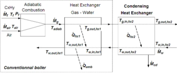
A model that predicts the boiler thermal performances and the condensing rate has been developed. It is similar to a conventional boiler model with a main counterflow gas-water heat exchanger, at which a condensing heat exchanger is added [7] (Figure 1).

Figure 1: Model structure

The first part of the model is an adiabatic combustion zone, where the combustion process is considered. Reactants are fictitiously brought to the reference temperature at which the heating value of the fuel is defined. As the chemical reaction between the reactants takes place, the heat is released and is used to heat the

combustion products to the final temperature Tadiab. Knowing the oxygen content in the flue gas and the fuel

composition, the energy conservation relationship is applied and the adiabatic temperature is calculated as well as the combustion products composition. Notice that a complete combustion is assumed.

After the combustion zone, the combustion products enters the main heat exchanger at the adiabatic temperature where the heat transfer takes place by radiation and convection. This heat exchanger is supposed to be a

counter-flow heat exchanger and the heat transfer between the flue gases and the water is calculated by the classical ε

-NTU method. The exact geometry of boilers is generally unknown by the users so that the heat transfer from the combustion products cannot be calculated using conventional radiation and convection relationships. To simplify

the calculation, a global heat transfer coefficient UAHX1 is defined, that is a function of the injected power and

the global air excess. This coefficient is evaluated from a nominal set point using Eq.(1) [8].

67 , 0 , , 1 1

















=

M

M

UA

UA

&

&

Heat transfer in a boiler firebox mainly occurs by radiation. Considering that combustion gases enter the main heat exchanger at adiabatic temperature is a simplification that could introduce an error as Eq. (1) mainly considers convection. This error can be reduced if another parameter is introduced on the flame temperature as it is done in [9]. Bourdhouxhe et al. [7] define a secondary heat exchanger to take into account heat loss of the water body of the boiler to the ambient. Modern boilers are very well insulated and experimental evaluation of this loss is hard to achieve. This secondary heat exchanger is neglected in the model developed in this work as this loss is negligible compared to the heat loss from the flue gas at the chimney.

After the main heat exchanger, the flue gas temperature is typically between 130°C and 180°C. In the model it is first converted into equivalent wet air according to Eq.(2) and Eq.(3). In this way, the wet heat exchanger is simulated by an air conditioning heat exchanger (the cooling coil), which currently handles latent as well as sensible heat transfer.

2 , 2 , 2 ,hx ahx ahx g g

c

M

c

M

&

=

&

M

M

M

&

ω

=

&

+

&

ω

Hanby [6] also presented a method using a cooling coil to model the condensing heat exchanger but the main difference with Hanby's model lies in the cooling coil model. Here, the coil is divided into smaller parts and each part is simulated by a model presented by Morisot [10], which calculates fluids output conditions and the cooling coil performances from a nominal set point. The condensing heat exchanger can operate either in totally dry regime, in totally wet regime, or in partially wet regime. In the case of a partially wet regime, two different calculations are done. The first calculation supposes that the cooling coil is totally dry and the second supposes that the cooling coil is completely wet. The solution that is chosen is the one that gives the largest heat transfer. This hypothesis was proposed by Braun [11] because, in case of combined wet and dry regimes, either assuming a dry or wet regime lowers the actual heat transfer. If the dry assumption is taken, the latent heat transfer is not considered and the calculated heat transfer will be underestimated. If the completely wet assumption is taken, the heat transfer is also underestimated. In fact, in the part of the coil that is dry, the model "humidifies" the air and the latent heat transfer to the air associated with this fictitious mass transfer reduces the overall calculated cooling capacity. Braun mentions that this assumption introduces an error smaller than 5%. The boiler condensing heat exchanger has been divided into five parts in order to reduce this error. In that way, the point where condensation appears is located on one element and the other elements work in completely wet or completely dry conditions. Morisot's model also assumed that the Lewis number is equal to the unity. This assumption has been checked for the equivalent humid air at the inlet conditions of the cooling coil. The diffusivity coefficient of humid air is evaluated with Chapman-Enskog theory [12]. It is showed that the Schmidt number is approximately equal to the Prandtl number (0.8); so that the Lewis number is around 1.

In short , there are six parameters to be determined experimentally. These parameters are mainly nominal flow rates and nominal heat transfer coefficients for both heat exchangers (Figure 2). The way that they are determined is described in the model validation for two specific boilers. The inputs and outputs of the model are shown on Figure 2. Knowing the reactants inlet conditions and the water inlet conditions, the boiler thermal efficiency is calculated as well as water and flue gas temperatures and condensed water flow rate.

Condensing Boiler Model Mw Tw,in,HX2 Pw Mf Tf [O2] Tamb RHamb Patm Pf Tw,out,HX1 Quseful Tg,out,HX2 η Mcd Fuel composition UAHX1,NMg,NUAw,NMw,NUAa,NMa,N PARAMETERS

Figure 2: Inputs and outputs of the model

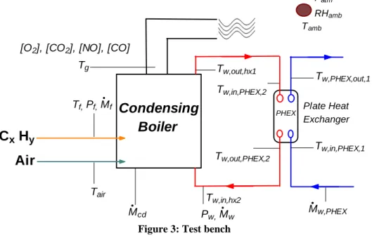
3. EXPERIMENTAL SETUP

Steady-state tests have been performed on two household boilers whose nominal output is 24 kW (a gas-fired boiler and a oil-fired boiler). A plate heat exchanger has been installed on the boiler loop in order to simulate the emitters of a house and regulate the return water temperature to the boiler (Figure 3). The useful power transferred to the water can be determined either with the measured data on the boiler closed loop or either with the measured data on the cooling side of the plate heat exchanger.

The natural gas composition that was used for the gas boiler is given in Table 1. Its lower heating value (LHV) is 45.10 MJ/kg and its higher heating value (HHV) is 49.91 MJ/kg at 25°C. Concerning the fuel oil used in the tests, its composition in weight is 13.1% of hydrogen and 86.9% of carbon. Its lower heating value is 42.86 MJ/kg and its higher heating value is 45.92 MJ/kg at 25°C.

Condensing

Boiler

Air

C

H

Tf, Pf, Mf T_w,out,hx1 Tw,in,hx2 Tw,in,PHEX,2 Tw,out,PHEX,2 Tw,PHEX,out,1 T_w,in,PHEX,1

PHEX Plate Heat

Exchanger Patm

RHamb

Tamb

P_w, M_w Mw,PHEX

Table 1: Natural gas composition xN2 0.028832 xCO2 0.018899 xCH4 0.87425 xC2H6 0.06126 xC3H8 0.01229 xC4H10 0.00313 xC5H12 0.00036 xC6H14 0.00083 xHe 0.0002

4. RESULTS AND ANALYSIS 4.1. Gas boiler parameters

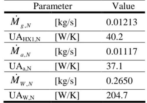
The first step to apply the model to the boiler is to determine the nominal parameters. Two tests were done for this purpose: one test in dry regime and one test in wet regime. The conditions to get a wet regime are met with the water return temperature to the boiler set at 30°C and 6% of oxygen in the flue gas. Another test is done in dry regime with a water return temperature to the boiler set at 53°C, the dew point of the water vapour in the flue gas is 52°C at this excess air. The value of the parameters are listed in Table 2. In this table, the nominal flue gas flow rate is the sum of the air flow rate and the natural gas flow rate at the nominal firing rate. The humid air mass flow rate is calculated with Eq.(2) and Eq.(3). The water mass flow rate does not vary into the boiler loop and is equal to 0.265 kg/s. To determine the nominal heat transfer coefficients, the error on the power transferred to the water is minimized. There are several solutions to the problem but the one that was chosen in this work is the one that minimize the error between the measured and the calculated combustion gas temperatures at the chimney. The number of elements in the condensing heat exchanger model has also been varied from 1 to 10 elements. It seems that it is no worth having a number of elements greater than 5.

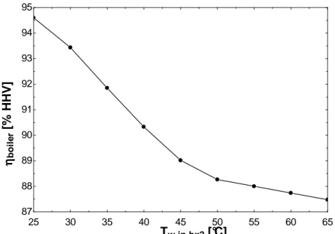
Once the parameters are fitted, the model behavior was checked by varying the water inlet temperature from 25°C to 65°C while keeping all other inputs constant (taken from the nominal tests conditions). The results are shown on Figure 4. The boiler thermal efficiency rises as the water temperature decreases. There is a sharp increase below the dew point. Figure 5 shows the thermal efficiency when the load varies. It can be seen on that figure that the boiler thermal efficiency increases as the firing rate decreases. This behavior was expected because the gas mass flow rate decreases so that the heat exchanger works more efficiently (increase of the flue gas residence time).

Table 2: Model parameters for the gas-fired boiler

Parameter Value N g

M

&

M

&

M

&

25 30 35 40 45 50 55 60 65 87 88 89 90 91 92 93 94 95 Tw,in,hx2 [°C] ηηηηbo il e r [ % H H V ]

Figure 4: Boiler thermal efficiency (on the higher heating value basis) as a function of the boiler inlet temperature for the gas-fired boiler working at full load and 6% of O2 in the flue gas

0.5 0.9 1.3 1.7 2.1 2.5 93 93.5 94 94.5 95 95.5 96 96.5 QNG [m³/h] ηηηηbo il e r [ % H H V ]

Figure 5: Boiler thermal efficiency (on the higher heating value basis) as a function of the firing rate for the gas-fired boiler at 6% of O2 in the flue gas and a return water temperature of 30°C.

4.2. Fuel oil boiler parameters

The fuel oil boiler parameters were determined in the same way as presented for the gas fired boiler, with one test in dry regime and one test in wet regime at 3% of oxygen at the stack. For fuel oil at this air excess, the dew point temperature of the water vapor in the flue gas is around 47°C. Thus, the return water temperature must be below 47°C to start to condensate. The main difference on the test bench compared to the gas-fired boiler is that the fuel oil boiler design permits to measure the fluids temperatures before and after the condensing heat exchanger. The parameters that were found are listed in Table 3. The boiler thermal efficiency curve has the

same shape than Figure 4 when the water inlet temperature is varied from 25°C to 65°C. The thermal efficiency (on the higher heating value basis) is 97% when the return water temperature is 25°C and decreases to 91% when the return water temperature is 65°C. Also, the boiler thermal efficiency decreases as the overall excess air

increases. It is equal to 96.5% and 93.5% for λ=1.05 and λ=2 respectively.

Table 3: Model parameters for the oil-fired boiler

Parameter Value N g

M

&

M

&

M

&

The simulated thermal performances have been compared to the experimental data for both boilers in order to validate the model. Tests have been performed in steady state conditions. The thermal efficiency of each boiler was measured by varying the return water temperature to the boiler. Moreover, the gas fired boiler allowed us to vary the firing rate whereas the oil fired boiler allowed us to vary the overall excess air.

The uncertainty on the measured thermal efficiency is estimated at around 2%. Globally, the model correctly estimates the boiler efficiency and the predicted values are within the measurement uncertainties for both boilers (Figure 6). Moreover, the model underestimates slightly the boiler exhaust flue gas temperature; the temperature difference is between 0°C and 4°C for both boilers.

20 25 30 35 40 45 50 55 84 86 88 90 92 94 96 98 100 Tw,in,hx2 [°C] ηηηηbo il e r [ % H H V ] ηboiler,Sim ηboiler,Sim ηboiler,Meas ηboiler,Meas 30 35 40 45 50 55 60 65 86 88 90 92 94 96 98 100 Tw,in,hx2 [°C] ηηηηbo il e r [ % H H V ] ηboiler,Sim ηboiler,Sim ηboiler,Meas ηboiler,Meas

Figure 6: Model boiler thermal efficiency compared to measured values at different boiler water inlet temperatures Left: for the gas-fired boiler – Right: for the oil-fired boiler

regimes by a reverse error on sensible heat. It seems also that, for dry regimes, the simulated efficiencies are greater than the measured ones. The results are mainly sensitive to an error on the nominal heat transfer coefficient of the heat exchanger HX1. The geometry of the tested boiler does not allow us to check the water and combustion gas temperature at this point, before the condensing heat exchanger.

At part load, the difference between the simulated and the measured efficiencies varies between 0.5% and 2% for a useful power of 15kW. The error on the flue gas temperature at this load is below 1°C and the condensate mass flow rate is estimated at 10%. At 10kW, the difference between the simulated and the measured efficiencies varies between 0.2% and 2.5%, which is slightly above the measurement uncertainty. The flue gas temperature is correctly estimated (below 1°C). 20 25 30 35 40 45 50 55 84 86 88 90 92 94 96 98 100 Tw,in,hx2 [°C] ηηηηbo il e r [ % H H V ] ηboiler,sim 15kW ηboiler,sim 15kW ηboiler,meas 10kW ηboiler,meas 10kW ηboiler,sim 24kW ηboiler,sim 24kW ηboiler,meas 24kW ηboiler,meas 24kW ηboiler,meas 15kW ηboiler,meas 15kW ηboiler,sim 10kW ηboiler,sim 10kW

Figure 7: Gas-fired boiler thermal efficiency at various firing rates and water inlet temperature – Comparison between measured and simulated results

For the fuel oil boiler, the simulated condensate mass flow rate is around 30% below the measured flow rate. The design of the boiler allow us to compare the calculated and simulated gas temperatures after both heat exchangers. The simulated gas temperature is on average 5°C above the measured one before the condensing heat exchanger and 2°C after the condensing heat exchanger (Figure 8).

0 50 100 150 200 250 25 30 35 40 45 50 55 60 65 Tw,in,hx2 [°C] T g ,o u t, h x 1 [ °C ] Tsim Tmeas 0 10 20 30 40 50 60 70 25 30 35 40 45 50 55 60 65 Tw,in,hx2 [°C] T g ,o u t, h x 2 [ °C ] Tsim Tmeas

Figure 8: Simulated temperature compared to the measured temperature at different boiler water inlet temperatures for the fuel oil boiler

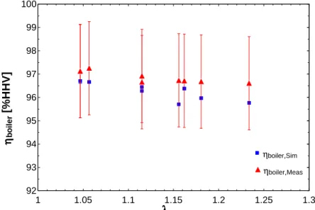
It seems that there is no significant thermal efficiency decrease when the amount of the combustion air increases on

the tested range. In fact, the efficiency difference between λ=1.05 and λ=1.24 is around 1%, which is lower than the

measurement uncertainty (±2%). 1 1.05 1.1 1.15 1.2 1.25 1.3 92 93 94 95 96 97 98 99 100 λλλλ ηηηηbo il e r [ % H H V ] ηboiler,Sim ηboiler,Sim ηboiler,Meas ηboiler,Meas

Figure 9: Oil-fired boiler thermal efficiency at different overall excess air for a return temperature of 30°C

5. CONCLUSION

A model that simulates the thermal performance in steady-state regime of a domestic natural gas or fuel oil-fired condensing boiler has been developed. Six parameters are needed for calculation. These parameters must be fitted with experimental data. The model was applied to two different household boilers whose nominal output is 24 kW. According to the experimental results, the model gives the correct trend for the boiler thermal efficiency. Regarding the estimation of the steam condensate mass flow rate, it seems that the latent heat transfer is underestimated and the sensible heat transfer overestimated in a way that the errors balance each other in wet regimes.

This model should be integrated into a building and HVAC simulation tool.

ACKNOWLEDGMENT

The financial support of the DG04 of the SPW (Walloon Region) is kindly acknowledged. The authors also want to acknowledge the company Viessmann for providing the tested boilers free of charge.

NOMENCLATURE

c Specific heat J/kg K

CxHy Hydrocarbons

CO Carbon monoxide concentration ppm

CO2 Carbon dioxide concentration %

LHV Lower Heating Value J/kg

NO Nitrogen monoxide concentration ppm

M& Mass flow rate kg/s

NTU Number of Transfer Units

O2 Oxygen concentration % P Pressure Pa Q Flow rate l/h Q& Power W RH Relative Humidity % T Temperature °C

UA Heat transfer coefficient W/K

x Molar fraction kmol CxHy / kmol fuel

Greeks letters

η Boiler thermal efficiency % on HHV basis

λ Air fuel equivalence ratio

ω Humidity ratio kg water/ kg dry air

Subscripts

1 Cold side of the plate heat exchanger

2 Hot side of the plate heat exchanger

a equivalent wet air

adiab adiabatic

air combustion air

amb ambient

atm atmospheric

cd condensate

f fuel

g combustion gas

hx1 main heat exchanger

hx2 condensing heat exchanger

in inlet conditions

meas measured value

N nominal value

NG Natural Gas

out outlet conditions

PHEX Plate Heat Exchanger

sim Simulated

v water vapour in the combustion products

w water

References

[1] M. Weiss, L. Dittmar, M. Junginger, M. K. Patel, and K. Blok, "Market diffusion, technological learning, and

cost-benefit dynamics of condensing gas boilers in the Netherlands," Energy Policy, vol. 37, pp. 2962-2976, 2009.

[2] D. Che, "Heat and mass transfer characteristics of simulated high moisture flue gases," Heat and mass transfer,

vol. 41, pp. 250-256, 2004.

condensing boiler," Energy Conversion and Management, vol. 45, pp. 3251-3266, 2004.

[4] Y. Liang, "Effect of vapor condensation on forced convection heat transfer of moistened gas," Heat and mass

transfer, vol. 43, pp. 677-686, 2007.

[5] D. Makaire and P. Ngendakumana, "MODELLING OF A DOMESTIC GAS-FIRED CONDENSING BOILER,"

presented at 30th TLM - IEA ENERGY CONSERVATION AND EMISSIONS REDUCTION IN COMBUSTION Capri, Italy, 2008.

[6] V. I. Hanby, " Modelling the performance of condensing boilers," Journal of the Energy Institute, vol. 80, pp.

229-231, 2007.

[7] J. Bourdouxhe, M. Grodent, J. Lebrun, and C. Saavedra, "A Toolkit for Primary HVAC System Energy

Calculation - Part 1: Boiler Model.," ASHRAE Transaction, vol. 100, pp. 759-773, 1994.

[8] O. Farias Fuentes, "Towards the Development of an Optimal Combustion Control in Fuel-Oil Boilers from the

Flame Emission Spectrum," in Faculté des Sciences Appliquées. Liège: Université de Liège, 1997.

[9] D. Makaire and P. Ngendakumana, "SIMULATION MODEL OF A SEMI-INDUSTRIAL FUEL OIL BOILER,"

presented at 5th European Thermal-Sciences Conference, Eindhoven, The Netherlands, 2008.

[10] O. Morisot, "Modèle de batterie froide à eau glacée adapté à la maîtrise des consommations d’énergie en

conception de bâtiments climatisés et en conduite d’installation," vol. Thèse de doctorat: Ecole des Mines de Paris, 2000.

[11] J. E. Braun, S. A. Klein, and J. W. Mitchell, "Effectiveness Models for Cooling Towers and Cooling Coils,"

ASHRAE Transactions #3270, vol. 95, Part 2, pp. 164-174, 1989.

[12] J. H. Lienhard IV and J. H. Lienhard V, A Heat Transfer Textbook, vol. Version 1.31, Third Edition ed.