University of Liege – ArGEnCo – Structural Engineering Institut de Mécanique et Génie Civil
Allée de la Découverte, 9 - 4000 Liège – Belgium Sart Tilman – Bâtiment B52 - Parking P52
www.argenco.ulg.ac.be
Validation of SAFIR
®
through
DIN EN 1992-1-2 NA
Comparison of the results for the examples
presented in Annex CC
March 2018
J. Ferreira
J.-M. Franssen
T. Gernay
A. Gamba
Table of contents
1. Introduction ... 3
1.1. Form of validation ... 3
1.2. Structure of the document ... 3
1.3. Sources of differences in results ... 3
1.4. Results versus visualisation ... 4
1.5. Versions of the software used ... 6
2. Validation examples ... 7
2.1. Example 1 – Heat transfer (cooling) with constant properties ... 7
2.2. Example 2 – Heat transfer (heating) with varying properties ... 19
2.3. Example 3 – Heat transfer through several layers ... 28
2.4. Example 4 – Thermal expansion ... 31
2.5. Example 5 – Temperature-dependent stress-strain curves of concrete and steel 37 2.6. Example 6 – Temperature-dependent limit-load-bearing capacity of concrete and steel 40 2.7. Example 7 – Development of restraint stresses ... 42
2.8. Example 8 – Weakly reinforced concrete beam ... 44
2.9. Example 9 – Heavily reinforced concrete beam ... 52
2.10. Example 10 – Reinforced concrete beam-column ... 58
2.11. Example 11 – Composite column with concrete cores ... 64
3. General conclusions ... 68
1. Introduction
1.1. Form of validation
Annex CC of DIN EN 1992-1-2 NA [2] presents a series of cases that allow benchmarking software tools aimed at the design of structures in a fire situation.
With the goal of providing a validation document for the finite element code SAFIR [1], a comparison of the reference results for the cases presented in the Annex CC with the results obtained by SAFIR has been carried out and is presented in this document.
The validation typically consists in a comparison between the value of a result (temperature, displacement or others) obtained by SAFIR and the value given as a reference and supposed to be the « true » result. The value obtained must fall in the interval stipulated by the document.
1.2. Structure of the document
This document contains comparisons of SAFIR with the examples provided by the DIN. For each example, keywords are initially provided in order to easily detect what is being analysed in the example. The objective of the example is then summarized and a description of the necessary information concerning geometry, boundary conditions, loads, parameters, material laws, etc, is given. Finally, a description of the model used and possible assumptions is presented and the main conclusions about the comparisons of SAFIR to the reference solutions are exposed.
All the SAFIR files used are made available with this document, and references to the folders where they are located are given in the sub-chapters related to each model. The pictures that allow visualizing the results of SAFIR were made with the post-processor DIAMOND 2016, which can be downloaded for free on the SAFIR website.
1.3. Sources of differences in results
Some differences between the results of SAFIR and the reference values may be observed either due to different formulations being used or to the way the results are obtained and presented. This is discussed in the next two sections.
1.3.1 Significant digits
In many cases, the true value is a real number and its expression should involve an infinite number of significant digits, like for instance 0,03458623579841265895123548… However, the determined value is always given with a certain resolution, i.e. a limited number of significant digits, and it is not always mentioned whether this has been obtained by rounding or by truncating the true value. In the example above, with only 2 significant digits, the rounded value is 0,035 whereas the truncated value is 0,0341. Such an uncertainty of 0,001 represents 2,857% of the
rounded value and 2,941% of the truncated value whereas the maximum allowed deviation may be as low as 1%.
Moreover, the results produced by SAFIR have by default a limited number of significant digits (typically 8 or 16 digits). As it may not be relevant to print all results with such a high
resolution, results are usually rounded before they are written in the two different files that are produced by SAFIR: filename.out and filename.xml. In these two files, the resolution may not be the same. For example, the displacements written in the out file, meant to be read by the human eye, are in 1/100 of a mm, which is supposed to be sufficiently small for a civil engineering structure. In the xml file, however, meant to be used by the graphic postprocessor Diamond, they are written with 3 significant digits.
In the exercises reported in this document, the values considered for SAFIR are always the most precise of both, based on the fact that any user has access to both files. For example, if the example above is a displacement in mm, SAFIR would write 0,00003 in the out file and 3,46E-03 in the xml file and the later would be used to calculate the deviation from the reference value. In this case, the double effect of rounding or truncating the reference value and of rounding the result of SAFIR would give a deviation of 1,14% with the rounded reference value and 1,76% with the truncated reference value, even if SAFIR calculates the true value to the 8th or 16th significant digit.
In some cases, it is possible to modify the size of the structure to be analysed in the reference case to obtain, at least, more significant digits in the out file produced by SAFIR. For example, the thermal expansion of a bar would be 10 times higher if the size of the bar is multiplied by 10. Interested users may want to do that, but this has not been done for this document.
1.3.2 Refinement of the model
The results calculated by a finite element software highly depend on the discretisation of the model in space, with finer grids yielding more correct results. If the analysis is transient, the results also depend on the discretisation in time, with smaller time steps yielding more correct results. The question of the discretisation to be used by the software, to produce the results that will be compared with the reference value, is typically not discussed in the documents that give the reference value.
In this exercise, the results are first presented with a model that is sufficiently refined (in space and in time) to ensure a converged solution, which means that the solution would not be different2 with a finer model. Yet, it is highly valuable for the user to have an idea of the
convergence of the solution when the model is “degraded”. This allows answering the following question: what level of refinement is required for the software to yield acceptable results? This is why for some of the examples, in addition to the results produced with the converged model, we will present also results obtained with different levels of refinement. It must then come as no surprise if, when the model is too crude, the results don’t fall within the acceptable limits anymore.
1.4. Results versus visualisation
Results produced by SAFIR come in the form of numbers. In order to validate the software, these numbers are considered and compared to the reference values and the results of the comparisons are usually given in tables. Yet, in order to give a more intuitive feeling of the results, these results can also be processed in order to create drawings. The graphical tool DIAMOND has
been specifically developed at Liege University to create drawings based on SAFIR results and has been used in this report3.
It has yet to be understood that some simplifications may be used to produce the drawings and these are discussed in this section.
1.4.1 Temperature field on triangular facets.
The temperature distribution on a triangular facet of a 3D SOLID element or on a triangular 2D SOLID element varies linearly. The graphic representation of the temperature distribution on such facets being linear is the exact representation of the temperature distribution considered in SAFIR, see Figure 12 for example.
The same holds for the representation of the warping function calculated for a torsion analysis.
1.4.2 Temperature field on quadrangular facets.
The temperature distribution on a quadrangular facet of a 3D SOLID element or on a quadrangular 2D SOLID element varies in a nonlinear manner. Being based on the temperature of the 4 nodes located at the corners of the facet, the temperature distribution is driven by an equation of the type given hereafter.
T(x,y) = k1 + k2 x + k3 y + k4 xy
In order to accelerate the drawings, this nonlinear distribution is simplified in DIAMOND. The temperature at the centre of gravity of the facet Tc is calculated exactly as the average of the
4 corner temperatures. Then DIAMOND divides the quadrangle into 4 triangles, each one based on the centre of the quadrangle and 2 adjacent corner nodes, see Figure 1. A linear temperature distribution is then assumed and drawn in each of the 4 triangles, and this distribution is different from the real distribution considered in SAFIR. This effect of artificial linearization is clearly visible, for example, on Figure 30 a) and Figure 31 a).
Figure 1 – Division of a quadrangle by DIAMOND
The same holds for the representation of the warping function calculated for a torsion analysis.
The visual effect of the approximation vanishes with the refinement of the mesh.
3 Any other graphical software could be used provided it can read the XML file produced by SAFIR.
1.4.3 Representation of deformed beam elements
Beam finite elements in the deformed configuration are curved, because the end nodes are subjected to a rotation with respect to the chord that joints them. Yet, in order to simplify and to accelerate the drawing process, DIAMOND will draw each beam finite element as a straight line between the end nodes. Here again, the drawn situation does not correspond exactly to the situation considered in SAFIR.
Figure 2 – Simplification of the drawn deformed configurations
In Figure 2, the thick curved line represents schematically a deformed configuration that could be considered by SAFIR whereas the two thin lines represent the configuration that would be drawn by DIAMOND for two beam finite elements.
Here also, the visual effect of the approximation vanishes with the refinement of the mesh.
1.5. Versions of the software used
The version of SAFIR used for performing the calculations was SAFIR 2016.c.0, whereas two different versions of DIAMOND2016 - versions v1.2.1.20 and v1.3.0.0 - were used for visualising the results and creating some of the illustrations presented in this document.
2. Validation examples
2.1. Example 1 – Heat transfer (cooling) with constant properties
2.1.1 Keywords
Heat-transfer, conduction, convection, constant thermal properties
2.1.2 Objective
The goal of this example is to analyse the heat transfer by conduction and convection in a 2D square section with constant thermal properties.
2.1.3 Description of the problem
A square section with the characteristics defined in Figure 1 and Table 1 is analysed. The temperature in the square section is uniform and equal to 1000°C at time t = 0 s when it is exposed to a gas with temperature = 0°C on one of the edges, the other edges being adiabatic. Heat transfer from the gas to the solid is by linear convection. In order to validate the results, the temperature θ0 calculated at the centre of the opposite edge, at point X, is compared to the reference values
presented in DIN EN1992-1-2 NA at different time instants.
Figure 3 – Example 1: Cooling down process in section with constant properties Table 1 – Dimensions, material properties and boundary conditions for Example 1
Properties Value Thermal conductivity λ W / (m∙K) 1 Specific heat cp J / (kg∙K) 1 Density ρ Kg / m3 1000 Dimensions h, b M 1 Coefficient of convection αc W / (m2∙K) 1 Emissivity εres = εm. εf - 0 Ambient temperature Θu °C 0
2.1.4 Model and results (see folder DIN1_4)
As the heat flow is uniaxial, from the exposed edge to the opposite edge, a model with only two rectangular elements on the width of the section is sufficient (in fact, a model with one single element on the width would yield the same answer, but it would not be possible to calculate the temperature at the centre node of the opposite edge). A structured mesh formed by 100 quadrilateral elements was used with 50 elements on the height, as depicted in Figure 4. Each of these elements contains 4 gauss points of integration (2x2) in its plane.
Figure 4 – Thermal model of the cross-section for Example 1 (2 x 50 SOLID elements) In SAFIR, a FRONTIER constraint with the function F0 was applied on the exposed edge, i.e. the lower edge in Figure 4 .
The PRECISION command was set to 1.0E-3. The material INSULATION, having constant material properties, was used and given the properties described in Table 1.
The time step chosen was 1 second (final time / 1800).
In Figure 5 is shown the distribution of the temperatures in the cross-section determined by SAFIR for the time t = 1800 s.
Table 2 shows the temperatures obtained by SAFIR and those given as reference by the DIN.
Table 2 – Temperatures Θ0 at point X for Example 1
Time Reference temperature Calculated temperature Deviation t Θ0 Θ'0 (Θ'0 - Θ0) (Θ'0 - Θ0) / Θ0 ∙ 100 s °C °C K % 0 1000 1000 0.00 0.00 60 999.3 999.20 -0.10 -0.01 300 891.8 891.80 0.00 0.00 600 717.7 717.78 0.08 0.01 900 574.9 574.99 0.09 0.02 1200 460.4 460.52 0.12 0.03 1500 368.7 368.84 0.14 0.04 1800 295.3 295.42 0.12 0.04 Limits ±5.00 ±1.00
It can be seen that the deviations fall well within the intervals of values defined in the DIN.
2.1.5 Analysis of the influence of different parameters
In this sub-chapter, an analysis of the sensibility of the results to different parameters is done. This will provide some indications on the minimum value of the time step or minimum number of nodes necessary in order to accurately simulate the cooling down process on the cross-section, as well as to confirm that the solution converges to a value as the mesh is refined.
2.1.5.1. Influence of the time step (see folder DIN1_5_1)
The mesh shown in Figure 5 was used here, and values of the time step equal to 1s, 5s, 10s, 20s, 30s, and 60s were tested. In Figure 4 are displayed the temperature distributions for four of these time steps, for the final time of 30min.
Figure 7 shows the evolution of the differences between the results from SAFIR and the ones of Annex CC as a function of time, depending on the value of the time step considered in the analysis.
a) 60s b) 30s c) 10s d) 1s
Figure 6 – Temperatures determined by SAFIR for some of the time steps tested, for t = 1800s (colour scale is the same as in Figure 5)
a) Percentage b) Degrees
Figure 7 – Differences between the results by SAFIR and the reference results for different time steps
Different observations can be made on the last Figure:
- Apart from the first 300s, the deviation is systematically positive; - After 600s, the deviation in terms of % increases linearly with time;
- The deviation in terms of K seems to remain more or less constant after 600s;
- Both criteria given in DIN are met as long as the time step does not exceed 25 s (final time/72). If only the absolute difference in K is considered, a time step of 40 s (final time/45) is acceptable.
-
2.1.5.2. Influence of the number of nodes (see folder DIN1_5_2)
To assess the influence of the refinement of the mesh on the results, different meshes, with still two elements on the horizontal direction but a varying number of elements on the direction of the heat flow, are analysed here considering analyses with a time step = 1s.
In Figure 8 are shown some of the meshes that were used. The temperatures determined after 30 min are plotted in Figure 9 for the meshes in Figure 8. The results for the deviations from the DIN found for all the meshes tested are presented in Figure 10.
-1.2 -0.8 -0.4 0.0 0.4 0.8 1.2 1.6 0 300 600 900 1200 1500 1800 Devia ti on [%] time [s]
Influence of the time step
60s 30s 20s 10s 5s 1s +1 % -1 % -6.0 -4.0 -2.0 0.0 2.0 4.0 6.0 8.0 0 300 600 900 1200 1500 1800 Devia ti on [K] time [s]
Influence of the time step
60s 30s 20s 10s 5s 1s +5 K -5 K
e) 2 x 2 (9 nodes) f) 2 x 8 (27 nodes) g) 2 x 20 (63 nodes) h) 2 x 100 (303 nodes) Figure 8 – Some of the meshes used in the study regarding the influence of the number of nodes on
the results a) 2 x 2 (9 nodes) b) 2 x 8 (27 nodes) c) 2 x 20 (63 nodes) d) 2 x 100 (303 nodes) Figure 9 – Temperatures determined by SAFIR for some of the meshes used to study the influence of
the number of nodes, for t = 1800s (colour scale is the same as in Figure 5)
a) Degrees b) P
Figure 10 – Deviations of the results by SAFIR from the reference results for quadrilateral meshes with different densities (expressed in number of nodes)
-6.0 -4.0 -2.0 0.0 2.0 4.0 6.0 8.0 10.0 12.0 14.0 0 300 600 900 1200 1500 1800 Dev iation [K] time [s]
Influence of the number of nodes
9 15 27 63 93 153 303 +5 K -5 K -1.2 -0.8 -0.4 0.0 0.4 0.8 1.2 1.6 0 300 600 900 1200 1500 1800 Devia ti on [%] time [s]
Influence of the number of nodes
9 15 27 63 93 153 303 +1 % -1 %
Figure 10 shows that the models have converged when having more than 27 nodes (i.e. 7 nodes on the depth of the model), and that the results are within the limits defined in the DIN for meshes with as few as 4 nodes on the depth (or 15 nodes in total), if a grid configuration with two elements on the width is respected.
2.1.5.3. Influence of the element type (see folder DIN1_5_3)
A study was done in order to understand how the utilisation of triangles can affect the results. With that purpose, the crudest mesh from Figure 8 was taken as reference and triangle meshes with identical number and distribution of nodes were tested. Again, the time step here considered was for all cases equal to 1s.
The results for the temperatures at the top edge nodes of the cross-section are shown in Figure 11 and Figure 12 for t = 1800s, for the quadrilateral mesh and the meshes with triangles, respectively.
Figure 11 – Temperatures determined by SAFIR at the top 3 nodes for a quadrilateral mesh with 2x2 elements (9 nodes), for t = 1800s
a) Mesh #1 b) Mesh #2 c) Mesh #3
Figure 12 – Temperatures determined by SAFIR at the top 3 nodes for three different triangle meshes with 9 nodes each for t = 1800s (colour scale is the same as in Figure 5)
It can be seen that for the three triangle meshes in Figure 12 the results depend on the
294.93 294.93 294.93
With a doubly symmetric mesh like the one in Figure 13, the same temperatures are obtained for the nodes with the same vertical position, as it is shown by the values plotted in that Figure for the top edge.
Figure 13 – Temperatures determined by SAFIR at the top 3 nodes for a doubly-symmetric triangle mesh with 13 nodes, for t = 1800s
Based on the latter, double symmetrical triangle meshes will be further compared to similarly refined models based on quadrilateral elements. For example, the triangle mesh in Figure 13 will be compared to the one presented in Figure 14.
Figure 14 – Temperatures determined by SAFIR at the top 3 nodes for a quadrilateral mesh with 15 nodes, for t = 1800s
Figure 15 and Figure 16 show all the meshes tested. The distribution of the temperatures in the cross-sections are plotted in Figure 17 for t = 1800s, and the results for the temperature at the studied point are plotted in Figure 18.
294.39 294.39 294.39
a) 13 nodes b) 23 nodes c) 43 nodes d) 83 nodes Figure 15 – Triangle meshes used to study the influence of the type of element on the results
a) 15 nodes b) 27 nodes c) 51 nodes d) 99 nodes
Figure 16 – Quadrilateral meshes used to study the influence of the type of element on the results
a) 13 nodes b) 23 nodes c) 43 nodes d) 83 nodes
Figure 17 – Temperatures determined by SAFIR for triangle meshes, for t = 1800s (colour scale is the same as in Figure 5)
a) Degrees b) Percentage
Figure 18 – Deviations of the results by SAFIR from the reference results for meshes with triangles and quadrilateral elements (expressed in number of nodes)
By observing the plots in Figure 18 one can see that, for the two crudest meshes related to each element type, the ones with quadrilaterals return the more accurate results and seem to converge faster to the solution implemented in SAFIR. However, this should be at least partially justified by the difference on the number of nodes between the models with quadrilaterals and triangles. As for the other meshes tested, it seems that for meshes with more than 23 nodes a convergence on the results is attained, regardless of the element type.
As for finding the crudest mesh able to return valid results according to the DIN, based on the plots above a mesh formed with triangles with slightly more than 13 nodes seems to be sufficiently refined for that purpose.
2.1.5.4. Influence of distorted meshes (see folder DIN1_5_4)
In order to understand what is the impact of the distortion of elements in the mesh, the 4 meshes present in Figure 19 and their undistorted counterparts in Figure 20 were analysed, considering a time step = 1s. The distribution of the temperatures in the cross-section is plotted in Figure 21 for t = 1800s, and the deviations of the results from the DIN with both types of meshes can be found in Figure 22.
a) 9 nodes b) 25 nodes c) 81 nodes d) 289 nodes
Figure 19 – Distorted meshes used to study the influence of distortion of elements on the results
-6.0 -4.0 -2.0 0.0 2.0 4.0 6.0 8.0 10.0 0 20 40 60 80 100 Devia ti on [K] number of nodes 300 s 300 s 1800 s 1800 s +5 K -5 K ∆ - triangles ⧠ - quadrilaterals -1.2 -0.8 -0.4 0.0 0.4 0.8 1.2 0 20 40 60 80 100 D evi ati on [% ] number of nodes 300 s 300 s 1800 s 1800 s +1 % -1 % ∆ - triangles ⧠ - quadrilaterals
a) 9 nodes b) 25 nodes c) 81 nodes d) 289 nodes Figure 20 – Undistorted meshes used to study the influence of distortion of elements on the results
e) 9 nodes f) 25 nodes g) 81 nodes h) 289 nodes
Figure 21 – Temperatures determined by SAFIR for the distorted meshes, for t = 1800s (colour scale is the same as in Figure 5)
a) Degrees b) Percentage
Figure 22 –Deviations of the results by SAFIR from the reference results for the distorted and undistorted meshes (expressed in number of nodes)
By looking at Figure 22 it is seen that by using distorted meshes the results deviate only slightly from the ones obtained with equivalent undistorted meshes.
-1.2 -0.8 -0.4 0.0 0.4 0.8 1.2 1.6 0 300 600 900 1200 1500 1800 Devia ti on [%] time [s]
Influence of having a distorted mesh
9 (dist.) 9 (undist.) 25 (dist.) 25 (undist.) 81 (dist.) 81 (undist.) 289 (dist.) 289 (undist.) +1 % -1 %
2.1.5.5. Influence of unstructured meshes (see folder DIN1_5_5)
As a last step of this parametric analysis, the influence of using unstructured meshes is investigated. The 6 unstructured meshes present in Figure 23 are analysed, again considering a time step = 1s. The distribution of the temperatures in the cross-section is plotted in Figure 24 for t = 1800s, and the deviations of the results from the DIN can be found in Figure 25.
a) 16 nodes b) 33 nodes c) 61 nodes
d) 90 nodes e) 117 nodes f) 141 nodes
Figure 23 – Meshes used to study the influence of unstructured meshes on the results
a) 16 nodes b) 33 nodes c) 61 nodes
d) 90 nodes e) 117 nodes f) 141 nodes
Figure 24 – Temperatures determined by SAFIR for the unstructured meshes, for t = 1800s (colour scale is the same as in Figure 5)
a) Degrees b) Percentage
Figure 25 –Deviations of the results by SAFIR from the reference results for the unstructured meshes (expressed in number of nodes)
One can observe from Figure 25 that:
- Overall, the results with unstructured meshes are well placed inside the stipulated values;
- Crude unstructured meshes like the one with 16 nodes therein present can lead to some deviations from the reference results (although relatively small);
- Unstructured meshes are less efficient and often require more nodes to attain the same level of results than structured ones, as it is proved by the fact that the unstructured mesh with 113 nodes in Figure 25 still presents some considerable deviations, whereas in Figure 22 a mesh with just 81 nodes was able to attain very close results to the ones found in the DIN;
- A very good agreement between the results from SAFIR and the DIN was achieved when using an unstructured mesh with 141 nodes.
2.1.6 Conclusions
The parametric analysis shows that the solution of SAFIR satisfies the requirement of the standard. The solution converges to the theoretical solution when the density of the mesh is increased and the value of the time step is reduced.
When refining the mesh, rectangular elements converge slightly faster than triangular element; regular structured meshes are most efficient, with slight differences being observed in distorted structured meshes; unstructured meshes are somehow less efficient while being still in the acceptable range of the standard.
-1.4 -1.0 -0.6 -0.2 0.2 0.6 1.0 0 300 600 900 1200 1500 1800 Devia ti on [%] time [s]
Influence of having a non-structured mesh
16 (unstr.) 33 (unstr.) 61 (unstr.) 90 (unstr.) 117 (unstr.) 141 (unstr.) +1 % -1 %
2.2. Example 2 – Heat transfer (heating) with varying properties
2.2.1 Keywords
Heat-transfer, conduction, convection, radiation, varying thermal properties
2.2.2 Objective
The goal of this example is to analyse the heat transfer by conduction when the thermal conductivity varies with the temperature, as well as the heat exchange with a gas at the boundary of the section by convection.
2.2.3 Description of the problem
A square section with the characteristics defined in Figure 26 and Table 3 is analysed. The temperature in the cross-section is uniform and equal to 0°C at time t = 0, when it is exposed to a gas with a temperature of 1000°C on all the edges. Heat transfer from the gas to the solid is by linear convection and radiation. In order to validate the results, the temperature θ0 calculated at
the centre of the cross-section is compared to the reference values presented in DIN EN1992-1-2 NA at different times, for a total duration of 3 hours.
Table 3 – Dimensions, material properties and boundary conditions for Example 2
Properties Value
Thermal conductivity λ (linear behaviour) W / (m∙K)
Θ λ (Θ) 0 1.5 200 0.7 1000 0.5 Specific heat cp J / (kg∙K) 1000 Density ρ Kg / m3 2400 Dimensions h, b mm 200 Coefficient of convection αc W / (m2∙K) 10 Emissivity εres = εm. εf - 0.8 Ambient temperature Θu °C 1000
Initial temperature in the cross-section Θcs °C 0
The data of this exercise are similar to that of a 20x20 cm² concrete section.
2.2.4 Model and results (see folder DIN2_4)
A model with a structured mesh formed by 576 square elements (24 by 24) was created. Each of these elements contains 2 gauss points of integration in its plane, and the total number of nodes is 625.
The initial temperature in the structure was set to 0°C, and a FRONTIER constraint of 1000°C was applied to all faces of the cross-section by the function “F1000”, as seen in Figure 27. The PRECISION command was set to 1.0E-3. A USER material was applied according to the properties described in Table 3. The time step chosen was 10 seconds (final time / 1080).
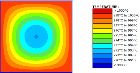
Figure 27 – Thermal model of the cross-section for Example 2 (24 x 24 SOLID elements) Figure 28 shows the temperature distribution for the final target time of 180 min.
Figure 28 – Temperatures determined by SAFIR for Example 2, for t = 180min
Table 4 gives the temperatures obtained by SAFIR and those given as reference by the DIN. All the differences are within the boundaries stipulated by the DIN.
Table 4 – Temperatures Θ0 for Example 2
Time Reference temperature Calculated temperature Deviation t Θ0 Θ'0 (Θ'0 - Θ0) (Θ'0 - Θ0) / Θ0 ∙ 100 min °C °C K % 30 36.9 32.18 -4.72 -12.79 60 137.4 132.40 -5.00 -3.64 Limit (t ≤ 60min) ±5.00 90 244.6 241.67 -2.93 -1.20 120 361.1 362.75 1.65 0.46 150 466.2 469.83 3.63 0.78 180 554.8 559.93 5.13 0.92 Limit (t > 60min) ±3.00
2.2.5 Analysis of the influence of different parameters
In this sub-chapter, an analysis of the sensibility of the results to different input parameters is done. This will provide some indications on the minimum value of the time step or minimum number of nodes necessary in order to accurately simulate the heating process on the cross-section, as well as to confirm that the solution converges to a value as the mesh is refined.
2.2.5.1. Influence of the time step (see folder DIN2_5_1)
To study the influence of the time step on the results, the mesh shown in Figure 27 was used, and values of the time step equal to 1, 5, 10, 20, 30, 60, 120, 300, 600 and 1200 s were tested.
Figure 29 shows the evolution of the differences between the results from SAFIR and the ones of Annex CC as a function of time, depending on the value of the time step considered in the analysis. The areas of the chart with a white background represent the domain where the criteria, either in terms of percentage or in degrees, must be applied.
a) Degrees b) Percentage
Figure 29 – Differences between the results by SAFIR and the reference results for different time steps
Different observations can be made on the last Figure:
- For the values of the time steps between 1s and 300s, inclusive, all the results fall within the intervals, considering the zones of application of each criteria (percentage or Kelvin degrees);
- When considering the absolute difference in Kelvin, considerable differences between the different time steps are obtained for t = 30 min, where bigger time steps consistently return bigger temperatures. For this time instant, the time step that returns a temperature value identical to the reference seems to be somewhere between 120s and 300s. For t = 60 min these differences practically disappear.
- For the range of application of the limit in percentage, the results provided are valid for time steps of less than 600s, inclusive, with bigger time steps consistently returning lower temperatures, contrary to what happens for the first 60 min.
-12.0 -7.0 -2.0 3.0 8.0 13.0 18.0 0 30 60 90 120 150 180 Devia ti on [K] time [min]
Influence of the time step
1800s 600s 300s 120s 60s 30s 20s 10s 5s 1s +5 K -5 K -8.0 -6.0 -4.0 -2.0 0.0 2.0 4.0 6.0 8.0 10.0 0 30 60 90 120 150 180 Devia ti on [%] time [min]
Influence of the time step
1s 5s 10s 20s 30s 60s 120s 300s 600s 1800s +3 % -3 %
2.2.5.2. Influence of the number of nodes (see folder DIN2_5_2)
To assess the influence of the refinement of the mesh on the results, 6 different meshes are analysed considering analyses with a time step = 10s. All meshes were defined as a grid with equal number of elements in each direction, respectively 2x2, 4x4, 8x8, 16x16, 24x24 and 50x50.
Figure 30 shows part of the meshes that are used. The temperatures determined after 180 min are plotted in Figure 31 for those meshes. The results for the deviations from the DIN found for all the meshes tested are presented in Figure 32.
a) 2 x 2 (9 nodes) b) 4 x 4 (25 nodes) c) 8 x 8 (81 nodes) d) 16 x 16 (289 nodes) Figure 30 – Meshes used to study the influence of unstructured meshes on the results
a) 2 x 2 (9 nodes) b) 4 x 4 (25 nodes) c) 8 x 8 (81 nodes) d) 16 x 16 (289 nodes) Figure 31 – Temperatures determined by SAFIR for some of the meshes used to study the influence
a) Degrees (overview) b) Percentage (overview)
c) Degrees (detailed view) d) Percentage (detailed view) Figure 32 – Differences between the results by SAFIR and the reference results for quadrilateral
meshes with different densities (expressed in number of nodes) The following comments can be made on Figure 32:
- The crudest meshes analysed returned results that are hugely and negatively affected by the skin effect – the use of a reduced number of consecutive linear functions as an approximation to a parabolic solution;
- Considering the stipulated boundaries, meshes with at least 625 nodes are able to provide valid results for the whole range of time steps analysed (this corresponds to element thickness of 8.3 mm);
- The mesh with 289 nodes (12.5 mm thick elements) is able to provide good results for the range covered by the limitation in terms of percentage, but not for the one in terms -800 -700 -600 -500 -400 -300 -200 -100 0 100 0 30 60 90 120 150 180 Devia ti on [K] time [min] 2601 625 289 81 25 9 +5 K -5 K -2500 -2000 -1500 -1000 -500 0 500 0 30 60 90 120 150 180 Devia ti on [%] time [min] 2601 625 289 81 25 9 +3 % -3 % -30 -25 -20 -15 -10 -5 0 5 10 0 30 60 90 120 150 180 Devia ti on [K] time [min]
Influence of the number of nodes
2601 625 289 81 25 9 +5 K -5 K -20 -15 -10 -5 0 5 0 30 60 90 120 150 180 Devia ti on [%] time [min]
Influence of the number of nodes
2601 625 289 81 25 9 +3 % -3 %
- It seems therefore as if 10 mm is approximately the limit for the thickness of element layers near the surface in concrete type sections.
2.2.5.3. Influence of the element type (see folder DIN2_5_3)
The influence of the type of element is analysed by means of 4 different triangle meshes compared with 4 quadrilateral meshes with a time step of 10 s.
Figure 33 and Figure 34 show the meshes tested. The distributions of the temperatures in the triangle meshes are plotted in Figure 35.
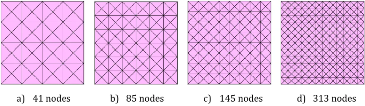
a) 41 nodes b) 85 nodes c) 145 nodes d) 313 nodes
Figure 33 – Triangle meshes used to study the influence of the type of element on the results
a) 81 nodes b) 169 nodes c) 289 nodes d) 625 nodes Figure 34 – Quadrilateral meshes used to study the influence of the type of element on the results
a) 41 nodes b) 85 nodes c) 145 nodes d) 313 nodes
Figure 35 – Temperatures determined by SAFIR for the triangle meshes, for t = 180 min (colour scale is the same as in Figure 28)
a) 30 and 60 min (in degrees) b) 90, 120, 150 and 180 min (in percentage)
Figure 36 – Deviations of the results by SAFIR from the reference results for meshes with triangles and quadrilateral elements (expressed in number of nodes)
From Figure 40 it can be seen that the difference in the results between triangular elements and square elements are not significant (marginally better results are obtained with square elements).
2.2.5.4. Influence of unstructured meshes (see folder DIN2_5_4 )
The influence of having unstructured meshes is investigated. The 4 meshes in Figure 37 were analysed, again considering a time step = 10s.
The distribution of the temperatures in the cross-section is plotted in Figure 38 for t = 180 min, and the deviations of the results from the DIN with the studied unstructured meshes are found in Figure 39.
a) 72 nodes b) 153 nodes c) 355 nodes d) 743 nodes Figure 37 – Meshes used to study the influence of unstructured meshes on the results
-100 -80 -60 -40 -20 0 20 0 100 200 300 400 500 600 700 Dev iation [K] number of nodes
Influence of the type of elements
30 min 30 min 60 min 60 min +5 K -5 K ∆ - triangles ⧠ - quadrilaterals -20 -15 -10 -5 0 5 0 100 200 300 400 500 600 700 Devia ti on [%] number of nodes 180 min 180 min 120 min 120 min 150 min 150 min 90 min 90 min +3 % -3 % ∆ - triangles ⧠ - quadrilaterals
a) 72 nodes b) 153 nodes c) 355 nodes d) 743 nodes Figure 38 – Temperatures determined by SAFIR for the unstructured meshes, for t = 180 min
(colour scale is the same as in Figure 28)
a) Degrees b) Percentage
Figure 39 – Differences between the results by SAFIR and the reference results, for quadrilateral meshes with different densities (expressed in number of nodes)
The analysis of the results in Figure 39 allows to conclude that having an unstructured mesh doesn’t greatly affect the results obtained, as a mesh with 743 nodes presents very identical results to the ones obtained with a structured mesh with 625 nodes (see Figure 33), which fall inside the DIN limits for all the range of time instants studied.
2.2.6 Conclusions
Like in Example 1, the parametric analysis has shown that the solution satisfies the requirement of the standard, provided that the mesh used is sufficiently refined.
It was noticed that meshes with quadrilateral elements converged slightly but not significantly faster than triangular elements, while no significant differences appeared between unstructured and structured meshes.
-40 -35 -30 -25 -20 -15 -10 -5 0 5 10 0 30 60 90 120 150 180 D evi ati on [K ] time [min]
Influence of the unstructured meshes
743 355 153 72 +5 K -5 K -40 -35 -30 -25 -20 -15 -10 -5 0 5 10 0 30 60 90 120 150 180 Dev iation [% ] time [min]
Influence of the unstructured meshes
743 355 153 72 +3 % -3 %
2.3. Example 3 – Heat transfer through several layers
2.3.1 Keywords
Heat-transfer, conduction, convection, radiation, various material layers
2.3.2 Objective
The goal of this example is to analyse the heat transfer in a steel hollow section that is filled with a lightweight insulating material. The thermal conductive properties of steel are those of EN 1993-1-2 whereas the filling material has constant thermal properties.
2.3.3 Description of the problem
A square section with the characteristics defined in Figure 40 and Table 5 is analysed. The temperature in the cross-section is uniform and equal to 0°C at time t = 0, when it is exposed to a gas with a temperature of 1000°C on all the edges. Heat transfer from the gas to the solid is by linear convection and by radiation. In order to validate the results, the temperature θ0 calculated
at the centre of the cross-section is compared to the reference values presented in DIN EN1992-1-2 NA, for a duration of 3 hours.
Legend: 1 Steel 2 Filling
Figure 40 – Example 3: Heat-transfer through several layers
Table 5 – Dimensions, material properties and boundary conditions for Example 3
Properties Steel Filling
Thermal conductivity λ W / (m∙K) EN 1993-1-2 0.05 Specific heat cp J / (kg∙K) EN 1993-1-2 1000 Density ρ Kg / m3 EN 1993-1-2 50 Dimensions h, b, t mm h = b = 201, t = 0.5 Coefficient of convection αc W / (m2∙K) 10 Emissivity εres = εm. εf - 0.8
2.3.4 Model and results (see folder DIN3_4)
A model with a structured mesh formed by 672 quadrilateral elements was created, which consists on a grid of 24 x 24 elements for the filling material, with the steel hollow section being defined with also 24 elements along each edge of the section and 1 element across the thickness. Each of these elements contains 2 Gauss points of integration, and the total number of nodes is 721.
The initial temperature in the structure was set to 0°C, and a frontier constraint of 1000°C was applied to all the faces of the cross-section according to Figure 41.
The PRECISION command was set to 1.0E-3. An INSULATION material with constant material properties according to Table 5 was used for the filling, and the STEELEC3EN material was used for the hollow section, by changing the heat transfer coefficients at the surface to match the values in Table 5. The time step chosen was 10 s (final time / 1080).
a) Overall view b) Detail of the two layers Figure 41 – Thermal model of the cross-section for Example 3 (24 x 24 SOLID elements)
Figure 42 shows the temperature distribution for the final time of 180min.
Figure 42 – Temperatures determined by SAFIR for Example 3, for t = 180min.
Table 6 shows the deviations of the temperatures obtained by SAFIR when compared to those given as reference by the DIN.
Table 6 – Temperature θ0 for Example 3
Time Reference temperature Calculated temperature Deviation t Θ0 Θ'0 (Θ'0 - Θ0) (Θ'0 - Θ0) / Θ0 ∙ 100 min °C °C K % 30 340.5 338.89 -1.61 -0.47 60 717.1 721.97 4.87 0.68 90 881.6 885.24 3.64 0.41 120 950.6 952.66 2.06 0.22 150 979.3 980.47 1.17 0.12 180 991.7 991.95 0.25 0.03 Limits ±5.00 ±1.00 2.3.5 Conclusions
The deviations found were within the limits stipulated by the DIN, both in absolute and in relative values, for the whole duration of the simulation.
2.4. Example 4 – Thermal expansion
2.4.1 Keywords
Thermal expansion, steel, homogenous temperature
2.4.2 Objective
The goal of this example is to analyse the thermal expansion of a steel member for different values of homogeneous temperature in a cross-section.
2.4.3 Description of the problem
A squared section with the characteristics defined in Figure 43 and Table 7 is analysed. In order to validate the results, the thermal elongation Δl at the simply supported end of the member is determined and compared to the reference values presented in DIN EN1992-1-2 NA.
Figure 43 – Example 4: Thermal expansion in statically assembled member Table 7 – Dimensions, material properties and boundary conditions for Example 4
Properties Steel
Dimensions l, h, b mm 100
Stress-strain material law EN 1993-1-2
Yield strength fyk N /mm2 355
Initial conditions °C 20
Homogeneous temperature in the member Θu °C 100, 300, 500, 600, 700, 900
Thermal expansion EN 1993-1-2
2.4.4 Model and results (see folder DIN4_4)
In this example the calculations were performed using BEAM 2D, BEAM 3D, TRUSS, SHELL and SOLID 3D elements, in order to get those different formulations validated.
No thermal analysis is presented here. The prescribed temperatures have been directly introduced in the relevant files for the structural analysis to be performed.
2D BEAM element
A 2D mechanical model with 1 BEAM element that is free to expand was created and exposed, unloaded, to the prescribed temperature fields.
In Figure 44 a representation of the thermal elongation determined by SAFIR is shown (in the Figure the elongation is causing the right support to move horizontally).
Figure 44 – Thermal elongation determined by SAFIR for Example4, for t = 900°C, using a 2D BEAM
element
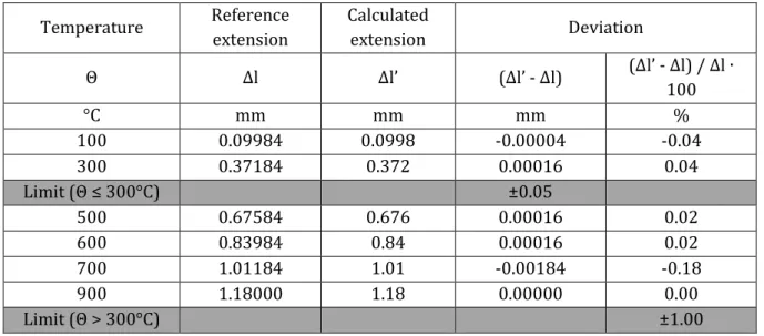
Table 8 shows the deviations of the temperatures obtained by SAFIR when compared to those given as reference by the DIN.
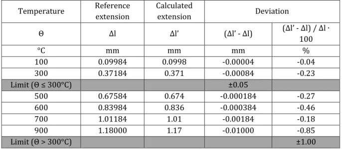
Table 8 – Thermal elongation Δl for Example 4, using a 2D BEAM element Temperature Reference extension Calculated extension Deviation Θ Δl Δl’ (Δl’ - Δl) (Δl’ - Δl) / Δl ∙ 100 °C mm mm mm % 100 0.09984 0.0998 -0.00004 -0.04 300 0.37184 0.372 0.00016 0.04 Limit (Θ ≤ 300°C) ±0.05 500 0.67584 0.676 0.00016 0.02 600 0.83984 0.84 0.00016 0.02 700 1.01184 1.01 -0.00184 -0.18 900 1.18000 1.18 0.00000 0.00 Limit (Θ > 300°C) ±1.00 3D BEAM element
A 3D mechanical model with 1 BEAM element that is free to expand was created and exposed, unloaded, to the prescribed temperature fields.
In Figure 45 a representation of the thermal elongation determined by SAFIR is shown (in the Figure the elongation is causing the support on the left to move according to the X-axis).
Figure 45 – Thermal elongation determined by SAFIR for Example 4, for t = 900°C, using a 3D BEAM element
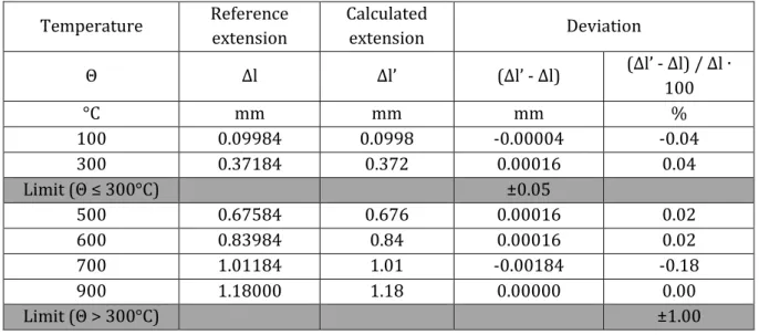
Table 10 shows the deviations of the temperatures obtained by SAFIR when compared to those given as reference by the DIN.
Table 9 – Thermal elongation Δl for Example 4, using a 3D BEAM element Temperature Reference extension Calculated extension Deviation Θ Δl Δl’ (Δl’ - Δl) (Δl’ - Δl) / Δl ∙ 100 °C mm mm mm % 100 0.09984 0.0998 -0.00004 -0.04 300 0.37184 0.372 0.00016 0.04 Limit (Θ ≤ 300°C) ±0.05 500 0.67584 0.676 0.00016 0.02 600 0.83984 0.84 0.00016 0.02 700 1.01184 1.01 -0.00184 -0.18 900 1.18000 1.18 0.00000 0.00 Limit (Θ > 300°C) ±1.00
TRUSS element
A 2D mechanical model with 1 TRUSS element that is free to expand was created and exposed, unloaded, to the prescribed temperature fields.
In Figure 46 a representation of the thermal elongation determined by SAFIR is shown (in the Figure the elongation is causing the right support to move horizontally).
Figure 46 – Thermal elongation determined by SAFIR for Example 4, for t = 900°C, using a TRUSS
element
Table 10 shows the deviations of the temperatures obtained by SAFIR when compared to those given as reference by the DIN.
Table 10 – Thermal elongation Δl for Example 4, using a BEAM element Temperature Reference extension Calculated extension Deviation Θ Δl Δl’ (Δl’ - Δl) (Δl’ - Δl) / Δl ∙ 100 °C mm mm mm % 100 0.09984 0.0998 -0.00004 -0.04 300 0.37184 0.371 -0.00084 -0.23 Limit (Θ ≤ 300°C) ±0.05 500 0.67584 0.674 -0.000184 -0.27 600 0.83984 0.836 -0.000384 -0.46 700 1.01184 1.01 -0.00184 -0.18 900 1.18000 1.17 -0.01000 -0.85 Limit (Θ > 300°C) ±1.00 SHELL element
A 3D mechanical model with 9 SHELL elements (3x3) that is free to expand was created and exposed, unloaded, to the prescribed temperature fields.
The visualization in DIAMOND of the displacements obtained by SAFIR in one of the directions is shown in Figure 47 (the same results were obtained for the expansion in both directions).
[m]
Figure 47 – Thermal elongation in Y-direction determined by SAFIR for Example 4, for t = 900°C,
using SHELL elements
Table 11 shows the deviations of the temperatures obtained by SAFIR when compared to those given as reference by the DIN.
Table 11 – Thermal elongation Δl for Example 4, using SHELL elements Temperature Reference extension Calculated extension Deviation Θ Δl Δl’ (Δl’ - Δl) (Δl’ - Δl) / Δl ∙ 100 °C mm mm Mm % 100 0.09984 0.0998 -0.00004 -0.04 300 0.37184 0.371 -0.00084 -0.23 Limit (Θ ≤ 300°C) ±0.05 500 0.67584 0.674 -0.000184 -0.27 600 0.83984 0.836 -0.000384 -0.46 700 1.01184 1.01 -0.00184 -0.18 900 1.18000 1.17 -0.01000 -0.85 Limit (Θ > 300°C) ±1.00 SOLID elements
A 3D mechanical model with 1 SOLID element that is free to expand was created and exposed, unloaded, to the prescribed temperature fields.
The visualization in DIAMOND of the displacements obtained by SAFIR in one of the directions is shown in Figure 48 (the same results were obtained for the expansion in all 3 directions).
[m]
Figure 48 – Thermal elongation in Y-direction determined by SAFIR for Example 4, for t = 900°C,
using a SOLID element
Table 12 shows the deviations of the temperatures obtained by SAFIR when compared to those given as reference by the DIN.
Table 12 – Thermal elongation Δl for Example 4, using a SOLID element Temperature Reference expansion Calculated expansion Deviation Θ Δl Δl’ (Δl’ - Δl) (Δl’ - Δl) / Δl ∙ 100 °C mm mm mm % 100 0.00984 0.0998 -0.00004 -0.04 300 0.37184 0.372 0.00016 0.04 Limit (Θ ≤ 300°C) ±0.05 500 0.67584 0.676 0.00016 0.02 600 0.83984 0.84 0.00016 0.02 700 1.01184 1.01 -0.00184 -0.18 900 1.18000 1.18 0.00000 0.00 Limit (Θ > 300°C) ±1.00 2.4.5 Conclusions
The results calculated for all types of elements are within the limits stipulated by the DIN. It may appear inconsistent that, in one single software, the thermal expansion is not exactly the same for all types of elements. Indeed, for 900°C, for example, the 2D BEAM, the 3D BEAM and the SOLID finite elements yield an expansion of 1.18 mm, which is exactly the expected value,
The reason lies in the fact that the axial strain is calculated based on a linearized expression in the SOLID elements (because they are written in a small displacements formulation) and in the BEAM finite elements (because these are expected to deflect essentially in bending rather than in elongation).
𝜀 = 𝑙 − 𝑙𝑖 𝑙𝑖
On the contrary, for the TRUSS elements where elongation is the sole deformation and in SHELL elements that can also work as membrane elements, the more correct nonlinear expression is being used.
𝜀 = 𝑙² − 𝑙𝑖² 2 𝑙𝑖²
It can be verified that, with an elongation of 1.17 mm from an initial length of 100 mm, the second expression yields a strain equal to 1.1768 %. If, by multiplying the length of the specimen by a factor of 10, one gains access to an additional significant digit, the elongation for the BEAM and the SOLID elements is found as 1.173 mm, which yields a strain of 1.1799 %.
The results are thus consistent with the fact that thermal strain of steel in SAFIR is calculated in the same manner for all element types, in full accordance with the recommendation of EN 1993-1-2.
2.5. Example 5 – Temperature-dependent stress-strain curves of
concrete and steel
2.5.1 Keywords
Elongation, column, steel, concrete, homogenous temperature
2.5.2 Objective
The goal of this example is to analyse the total elongation of a column made of steel or concrete for different uniform temperature distributions at some given stress-strength ratios.
2.5.3 Description of the problem
Members with the characteristics defined in Figure 49 and Table 13 are analysed. In order to validate the results, the elongation Δl at the unsupported end of the members is determined and compared to the reference values presented in DIN EN1992-1-2 NA.
Figure 49 – Example 5: Temperature-dependent stress-strain in column (stability failure is excluded)
Table 13 – Dimensions, material properties and boundary conditions for Example 5 and Example 6
Properties Steel Concrete a
Dimensions l, h, b mm 100, 10, 10 100, 31.6, 31.6
Stress-strain material law EN 1993-1-2 EN 1992-1-2
Yield strength fy (20°C) , fc (20°C) N/mm2 355 20
Thermal expansion EN 1993-1-2 EN 1992-1-2
Initial conditions °C 20
Homogeneous temperature in the
member Θ °C 20, 200, 400, 600, 800
Load σS (Θ) / fy (Θ) and σC (Θ) / fc (Θ) 0.2, 0.6, 0.9 a – with predominantly siliceous aggregates
2.5.4 Models and results (see folder DIN5_4)
A 2D mechanical model with 1 BEAM element was created and replicated in order to be associated to the 15 different combinations of the temperatures with the stress / strength ratios. Static analyses with a PRECISION of 10E-3s, a COMEBACK of 1s and a time step of 60s were performed for each case.
This was done for both steel and concrete using the materials STEELEC3EN and SILCONC_EN and the properties in Table 13. The results obtained are shown, respectively, in Table 14 and Table 15.
Table 14 – Elongation Δl for the steel column in Example 5 Temp. Stress / Strength Red. Coeff. Applied
force Ref. value
Calc. value Deviation Θ σSΘ / fyk(Θ) ky,θ = fy,θ/fy FcΘ Δl Δl’ (Δl’ - Δl) (Δl’ - Δl) / Δl ∙ 100 °C - - N mm mm mm % 20 0.2 1 -7100 -0.034 -0.0338 0.0002 -0.59 0.6 1 -21300 -0.101 -0.101 0.0000 0.00 0.9 1 -31950 -0.152 -0.152 0.0000 0.00 200 0.2 1 -7100 0.194 0.194 0.0000 0.00 0.6 1 -21300 0.119 0.119 0.0000 0.00 0.9 1 -31950 -0.159 -0.159 0.0000 0.00 400 0.2 1 -7100 0.472 0.472 0.0000 0.00 0.6 1 -21300 0.293 0.293 0.0000 0.00 0.9 1 -31950 -0.451 -0.451 0.0000 0.00 600 0.2 0.47 -3337 0.789 0.789 0.0000 0.00 0.6 0.47 -10011 0.581 0.581 0.0000 0.00 0.9 0.47 -15017 -0.162 -0.162 0.0000 0.00 800 0.2 0.11 -781 1.059 1.06 0.0010 0.09 0.6 0.11 -2343 0.914 0.915 0.0010 0.11 0.9 0.11 -3515 0.170 0.171 0.0010 0.59 Limit ± 3.00
Table 15 – Elongation Δl for the concrete column in Example 5 Temp. Stress / Strength Red. Coeff. Applied
force Ref. value
Calc. value Deviation Θ σSΘ / fyk(Θ) fc,θ/fck FcΘ Δl +Δl’ (Δl’ - Δl) (Δl’ - Δl) / Δl ∙ 100 °C - - N mm mm mm % 20 0.2 1 -3994 -0.0334 -0.0334 0.0000 0.00 0.6 1 -11983 -0.104 -0.104 0.0000 0.00 0.9 1 -17974 -0.176 -0.176 0.0000 0.00 200 0.2 0.95 -3795 0.107 0.107 0.0000 0.00 0.6 0.95 -11384 -0.0474 -0.0474 0.0000 0.00 0.9 0.95 -17075 -0.2075 -0.207 0.0005 -0.24 400 0.2 0.75 -2996 0.356 0.356 0.0000 0.00 0.6 0.75 -8987 0.075 0.075 0.0000 0.00 0.9 0.75 -13481 -0.216 -0.216 0.0000 0.00 600 0.2 0.45 -1797 0.685 0.685 0.0000 0.00 0.6 0.45 -5392 -0.0167 -0.0167 0.0000 0.00 0.9 0.45 -8088 -0.744 -0.744 0.0000 0.00 800 0.2 0.15 -599 1.066 1.07 0.0040 0.38 0.6 0.15 -1797 0.365 0.365 0.0000 0.00 0.9 0.15 -2696 -0.363 -0.363 0.0000 0.00 Limit ± 3.00 2.5.5 Conclusions
For both steel and concrete, the major part of the cases returned exactly the same value as the reference. Whenever this was not the case, the differences found were minor and well within the boundaries stipulated by the DIN, and those were related to the number of significant digits produced by SAFIR in .xml file and displayed in DIAMOND.
Calculations were also performed using the TRUSS and the BEAM 3D elements, for the cases with 600°C and a stress / strength ratio of 0.6, which returned the same (or virtually the same) results as for the BEAM 2D cases, for both steel and concrete.
2.6. Example 6 – Temperature-dependent limit-load-bearing capacity
of concrete and steel
2.6.1 Keywords
Ultimate bearing capacity, column, steel, concrete, homogeneous temperature
2.6.2 Objective
2.6.3 Description of the problem
Members with the characteristics defined in Figure 49 and Table 13 are analysed. In order to validate the results, the load bearing capacity of the members is determined and compared to the reference values presented in DIN EN1992-1-2 NA.
2.6.4 Models and results (see folder DIN6_4)
The same models of the previous example were used, but the tem files were modified and a new custom load function named “fload.fc” was introduced, in order to allow for a phase where the cross-section is heated without load for 512s until it reaches the target temperature, and another phase where the load is increased at constant temperature until the failure of the column. One single beam element was used, which does not allow buckling of the columns to develop. This decision is motivated by the low slenderness of the columns that are proposed, which seems to indicate that this example has been designed with validation of the material laws in mind, more than the validation of a structural behaviour. The good match that will be observed between the calculated results and the reference results seems to confirm that this was indeed the case.
The results for the differences in the ultimate resistances obtained in static analyses performed by SAFIR and the reference results are presented in Table 16 and Table 17.
Table 16 – Ultimate resistance of the steel member in Example 6 Temperature Reference force Calculated force Deviation
Θ NRk.fi N’Rk.fi (N'Rk,fi,k - NRk,fi,k) (N'Rk,fi,k - NRk,fi,k)
/ NRk,fi,k ∙ 100 °C kN kN kN % 20 -35.5 -35.5 0.0 0.00 200 -35.5 -35.5 0.0 0.00 400 -35.5 -35.5 0.0 0.00 600 -16.7 -16.7 0.0 0.00 800 -3.9 -3.9 0.0 0.00 Limits ± 0.5 ± 3.00
Table 17 – Ultimate resistance of the concrete member in Example 6 Temperature Reference force Calculated force Deviation
Θ NRk.fi N’Rk.fi (N'Rk,fi,k - NRk,fi,k) (N'/ NRk,fi,k - NRk,fi,k)
Rk,fi,k ∙ 100 °C kN kN kN % 20 -20 -20.0 0.0 0.00 200 -19 -19.0 0.0 0.00 400 -15 -15.0 0.0 0.00 600 -9 -9.0 0.0 0.00 800 -3 -3.0 0.0 0.00 Limits ± 0.5 ± 3.00
2.6.5 Conclusions
A perfect agreement between the expected results and the ones obtained by SAFIR was found for all the cases considered, using the 2D BEAM elements.
Calculations were also performed using the TRUSS and the BEAM 3D elements, for the cases with 600°C, which returned the same (or virtually the same) results as for the BEAM 2D cases, for both steel and concrete.
2.7. Example 7 – Development of restraint stresses
2.7.1 Keywords
Thermal induced forces, steel, homogenous temperature, varying temperature
2.7.2 Objective
The goal of this example is to determine the thermal induced internal forces and stresses for a fixed-fixed steel beam, for two different temperature distributions: one constant and one that varies linearly on the depth of the cross-section.
2.7.3 Description of the problem
The members with the characteristics defined in Figure 50 and Table 18 are analysed. In order to validate the results, the values of the internal axial and bending forces and the stresses at the bottom of the cross-section are determined for the two temperature distributions and compared to the reference values presented in DIN EN1992-1-2 NA.
Table 18 – Dimensions, material properties and boundary conditions for Example 7
Properties Steel
Dimensions l, h, b mm 1000, 100, 100
Stress-strain material law EN 1993-1-2
Yield strength fy N /mm^2 650 a Elastic modulus Ea (20°C) N / mm^2 210 000 Thermal expansion EN 1993-1-2 Temperature of the member Θo °C 120 20 Θu °C 120 220
a - Structural steel according to DIN EN 1993-1-1 using the notional yield fy (20 ° C) = 650 N / mm2 (no high-strength steel) and the thermo-mechanical properties according to DIN EN 1993-1-2
2.7.4 Models and results (see folder DIN7_4)
Two .tem files were created with 20 fibres of 5 mm depth equally distributed on the depth of the section. The temperature of 120°C was assigned to all fibres in the first file. In the second file, the temperature varied linearly from 25°C in fibre 1 to 215°C in Fibre 20.
Figure 51 – Cross-section used for Example 7 (20 fibres)
A 2D mechanical model with 1 BEAM element was created and duplicated in order to be associated to the 2 different temperature distributions. STATIC analyses using a PURE_NR (pure Newton-Raphson) procedure, with a PRECISION of 10-3s and a time step of 1s were performed
Table 19 – Internal forces and stresses due to thermal expansion for Example 7
Temp. Parameter Reference Calculated Deviation
Limits Θ0 | Θu Desig. Units X X’ (X’ – X) / X ∙ 100 °C % % 120 | 120 Nzw kN -2585 -2584.8 -0.01 ± 1.00 Mzw kN.m 0 0 0.00 ± 1.00 σzw N / mm2 -258.5 -258 -0.19 ± 5.00 20 | 220 Nzw kN -2511 -2510.6 -0.02 ± 1.00 Mzw kN.m -40.3 -40.207 -0.23 ± 1.00 σzw N / mm2 -479 -469 -2.09 ± 5.00 2.7.5 Conclusions
A good agreement between the reference results and the ones obtained by SAFIR was found for the results for both the cases.
It has to be mentioned that the stresses were determined for the fibres at the bottom of the cross-section and hence their value do not correspond precisely to the value at the bottom edge, but to the centre of the fibre. This is the cause of the difference of 2% found for the 20|220 case. The difference for this case will be reduced if a thinner fibre is considered at the edge of the section. For instance, if a mesh with 200 fibres of equal size is considered, the stress determined by SAFIR at the bottom fibre is 478 N/mm2, hence much closer to the 479 N/mm2 presented in
DIN.
2.8. Example 8 – Weakly reinforced concrete beam
2.8.1 Keywords
Fire resistance time, weakly reinforced concrete beam, ISO fire curve
2.8.2 Objective
Example 8 deals with a weakly reinforced concrete beam with a uniform distributed load that is subjected to the standard fire on three sides. The goal is to determine the requested area for the two steel rebars in order to provide a fire resistance of 90 minutes to the beam.
2.8.3 Description of the problem
The member with the characteristics defined in Figure 52 and Table 20 is analysed. The required value for the steel area to ensure that the beam reaches 90 min of resistance when subjected to an ISO fire is determined and compared to the reference value presented in DIN EN1992-1-2 NA.
[cm]
Figure 52 – Example 8: Cross-section and configuration of the weekly reinforced concrete beam Table 20 – Dimensions, material properties and boundary conditions for Example 8
Fire resistance category R90
Dimensions l, b , h mm 3000, 200, 380
Spacing a, as mm 45, 55
Loads qE,fi,d,t kN/m 29
Concrete C20/25 fc (20°C) N/mm2 20
Moisture content (by mass) w % 3
Steel B500 fy (20°C) N/mm2 500
Stress-strain material law Concrete a EN 1992-1-2
Rebars b
Fire exposure ISO 834 (three sides) EN 1991-1-2
Coefficient of convection αc W/(m2.K) 25
Emissivity εm 0.7
Thermal and physical material properties
Concrete λ, ρ, cp, εth,c EN 1992-1-2
Steel λa, ρ, ca, εth,s EN 1994-1-2
a – with predominantly siliceous aggregates and density ρ = 2400 kg/m3 b – class N, hot-rolled
2.8.4 Models and results (see folder DIN8_4)
Different models of the section were created, by changing the area of the two steel bars from one model to another (see Figure 53). The ISO fire curve was applied on 3 sides of the section while the upper side was adiabatic.
a) Overall view b) Detail of one of the rebars Figure 53 – Example of one of the thermal models of the cross-section tested for Example 8
The whole length of the beam was modelled with 20 2D BEAM finite elements of equal length (see Figure 54).
Figure 54 – Structural model of the beam (20 BEAM elements of equal sizes)
Steel was modelled by the material STEELEC2EN, with the fabrication process HOTROLLED and with the ductility class B (no mention to the ductility class is given in DIN but this was found to be the one resulting in better approximations to the results in DIN).
Concrete was modelled by the material SILCONC_EN. In thermal analysis, the upper limit for the thermal conductivity, found in clause 3.3.3 of EN1992-1-2, was considered, since this is this one recommended by Eurocode and that led to better approximations to the results in DIN.
The calculations performed were DYNAMIC and used the PURE_NR (pure Newton-Raphson) procedure. The initial time step was set to 1s, the maximum time step to 60s, the PRECISION to 10E-3s, and the COMEBACK to 0.01s.
The fire resistance times obtained in the mechanical analyses, corresponding to the last converged time step, were observed for each section used. It was found that a diameter for each
The temperature in the rebars and the fire resistance times obtained for the different iterations made are shown in Figure 55.
Figure 55 – Evolution of the temperature at the centre of the rebars and of the fire resistance with the steel area
The temperature distribution after 90 minutes, in the section with A’s = 3.29 cm2, is shown
in Figure 56.
Figure 56 – Temperatures determined by SAFIR for t = 90 min, for Example 8, with two rebars of 14.47mm (bottom part of the model)
Figure 57 shows the evolution of the vertical displacement at mid-span of the beam. The vertical displacement at the last converged time is 106 mm, corresponding to l/28.3. The horizontal inward displacement on the right hand support is 28.1 mm for the same time instant.
530 535 540 545 550 555 560 565 570 3 3.1 3.2 3.3 3.4 3.5 3.6 3.7 T em perature in r ebars [° C] Area of steel [cm2]
Temperature in rebars vs area of steel
DIN SAFIR -10 % A s 3.56 cm 2 3.29 cm 2 3 3.1 3.2 3.3 3.4 3.5 3.6 3.7 86 87 88 89 90 91 92 93 94 95 96 Area of steel [cm2] Fi re res is tan ce ti m e [mi n.]
Fire resistance time vs area of steel
DIN SAFIR 90 min -10 % A s 3.29 cm 2 3.56 cm 2
Figure 57 – Vertical displacement vs. time at mid-span of the beam obtained by SAFIR The results obtained with SAFIR, as well as the reference values of DIN EN1992-1-2 NA, are summarized in Table 21.
Comments on the results obtained will be given at the last part of this example.
Table 21 – Necessary area of steel to resist an ISO fire for 90 min, for the weekly reinforced concrete beam in Example 8
Temperature in the
rebars for t = 90 min Area of the steel rebars Fire
resistance class
Reference Calculated Reference Calculated Deviation
Limit
T T’ As A’s (A’s – As) /
As.100
°C °C cm2 cm2 % %
R90 562 544 3.56 3.29 -7.61 ± 10.00
2.8.5 Analysis of the influence of different parameters in the structural analysis
An analysis of the sensibility of the results to different parameters is done, which will provide indications on the influence of the type of analysis, on the minimum value of the time step or the minimum number of BEAM elements necessary to accurately simulate the mechanical behaviour of the beam, and to confirm that the solution converges to a value as the mesh is refined. The thermal model with the area of steel of 3.29 cm2 mentioned above was used in all the
analyses.
2.8.5.1. Influence of the type of analysis (see folder DIN8_5_1)
tested in a STATIC and in a DYNAMIC analysis. For the DYNAMIC analyses, three values for the mass were used: 0 kg/m; 190 kg/m (the mass of the beam); and 2090 kg/m (the mass of the beam plus the mass of the gravity load).
The results obtained allow to conclude that, for the current example, the type of analysis and type of procedure chosen don’t affect the results, regardless of the value given for the MASS (in DYNAMIC analyses).
Table 22 – Fire resistance times obtained with different analysis options, for Example 8
Case Type of analysis MASS Fire resistance time
Name
Type Procedure kg/m min
DIN8_5_1( ) a STATIC PURE_NR - 90.5 b APPR_NR - 90.5 c DYNAMIC PURE_NR 0 90.5 d* 190 90.5 e 2090 90.5 f APPR_NR 0 90.5 g 190 90.5 h 2090 90.5
*same case as the one tested before in 2.8.4
2.8.5.2. Influence of the time step (see folder DIN8_5_2)
To study the influence of the time step on the results, the same model was used, and values of the time step equal to 5, 10, 30, 60, 120, 300 and 600 s were tested. Two types of analysis, one STATIC and one DYNAMIC with the MASS of 190 kg/m, were performed. The results are shown in Table 23.
Table 23 – Fire resistance times obtained with different time steps, for the two types of analysis, for Example 8
Case STATIC analysis DYNAMIC analysis
DIN8_5_2( ) Time step
Fire resistance time Initial time step Maximum time step Fire resistance time s min s s min a 5 90.5 5 30 90.5 b 10 90.5 5 60 90.5 c 30 90.5 5 120 90.5 d 60 90.5 5 300 90.5 e 120 90.5 5 600 90.5 f 300 90.5 30 600 90.5 g 450 90.5 60 600 90.5 h 600 90.5 300 600 90.5 i 1200 90.5 600 600 90.5