SIMULATEUR TUTORIEL INTELLIGENT POUR
LES OPERATIONS ROBOTISEES
APPLICATION AU BRAS CANADIEN SUR LA STATION
SPATIALE INTERNATIONALE
par
Khaled Belghith
These presentee au Departement d'informatique
en vue de l'obtention du grade de philosophise doctor (Ph.D.)
FACULTE DES SCIENCES
UNIVERSITE DE SHERBROOKE
1 * 1
Canada Archives Canada Library and Archives Bibliothfeque et Published Heritage Direction duBranch Patrimoine de l'6dition 395 Wellington Street Ottawa ON K1A 0N4 Canada 395, rue Wellington Ottawa ON K1A 0N4 Canada
Your file Votre r6ference ISBN: 978-0-494-70601-5 Our file Notre r6f6rence ISBN: 978-0-494-70601-5
NOTICE:
The author has granted a
non-exclusive license allowing Library and Archives Canada to reproduce, publish, archive, preserve, conserve, communicate to the public by
telecommunication or on the Internet, loan, distribute and sell theses
worldwide, for commercial or non-commercial purposes, in microform, paper, electronic and/or any other formats.
AVIS:
L'auteur a accorde une licence non exclusive permettant a la Bibliotheque et Archives Canada de reproduire, publier, archiver, sauvegarder, conserver, transmettre au public par telecommunication ou par I'lnternet, preter, distribuer et vendre des theses partout dans le monde, a des fins commerciales ou autres, sur support microforme, papier, electronique et/ou autres formats.
The author retains copyright ownership and moral rights in this thesis. Neither the thesis nor substantial extracts from it may be printed or otherwise reproduced without the author's permission.
L'auteur conserve la propriete du droit d'auteur et des droits moraux qui protege cette these. Ni la these ni des extraits substantiels de celle-ci ne doivent etre imprimes ou autrement
reproduits sans son autorisation.
In compliance with the Canadian Privacy Act some supporting forms may have been removed from this thesis.
While these forms may be included in the document page count, their removal does not represent any loss of content from the thesis.
Conformement a la loi canadienne sur la protection de la vie privee, quelques formulaires secondaires ont ete enleves de cette these.
Bien que ces formulaires aient inclus dans la pagination, il n'y aura aucun contenu manquant.
1 * 1
Le 22 juillet 2010,
le jury a accepte la these de Monsieur Khaled Belghith dans sa version finale.
Membres du jury
Professeur Froduald Kabanza Directeur de recherche Departement d'informatique
Professeur Roger Nkambou Membre
Departement Informatique Universite du Quebec a Montreal
Docteur Leo Hartman Membre externe Agence spatiale canadienne
Professeur Richard St-Denis President rapporteur Departement d'informatique
Sommaire
Cette these a pour objectif de developper un simulateur tutoriel intelligent pour l'ap-prentissage de manipulations robotisees, applicable au bras robot canadien sur la station spatiale internationale. Le simulateur appele Roman Tutor est une preuve de concept de simulateur d'apprentissage autonome et continu pour des manipulations robotisees com-plexes. Un tel concept est notamment pertinent pour les futures missions spatiales sur Mars ou sur la Lune, et ce en depit de l'inadequation du bras canadien pour de telles missions en raison de sa trop grande complexity. Le fait de demontrer la possibilite de conception d'un simulateur capable, dans une certaine mesure, de donner des retroactions similaires a celles d'un enseignant humain, pourrait inspirer de nouvelles idees pour des concepts similaires, applicables a des robots plus simples, qui seraient utilises dans les prochaines missions spatiales. Afin de realiser ce prototype, il est question de developper et d'inte-grer trois composantes originales : premierement, un planificateur de trajectoires pour des environnements dynamiques presentant des contraintes dures et flexibles ; deuxiemement, un generateur automatique de demonstrations de taches, lequel fait appel au planificateur de trajectoires pour trouver une trajectoire solution a une tache de deplacement du bras robot et a des techniques de planification des animations pour filmer la solution obtenue; et troisiemement, un modele pedagogique implementant des strategies d'intervention pour donner de l'aide a un operateur manipulant le SSRMS. L'assistance apportee a un opera-teur sur Roman Tutor fait appel d'une part a des demonstrations de taches generees par le generateur automatique de demonstrations, et d'autre part au planificateur de trajectoires pour suivre la progression de l'operateur sur sa tache, lui fournir de l'aide et le corriger au besoin.
Remerciements
A mon directeur de these, monsieur Froduald Kabanza, professeur au departement d'in-formatique de l'Universite de Sherbrooke. Je vous remercie de m'avoir accueilli dans votre laboratoire et de m'avoir confie ce projet qui me tenait particulierement a coeur. Puissent ces quelques mots vous temoigner de ma profonde gratitude, pour votre encadrement exem-plaire, votre soutien, votre confiance, ainsi que pour vos precieux apports scientifiques tout au long de cette these.
A tous les membres du jury de cette these. Je vous remercie vivement pour l ' h o n n e u r que vous me faites en acceptant d'evaluer ce travail de recherche.
A monsieur Roger Nkambou, professeur a l'Universite du Quebec A Montreal. Un grand Merci pour votre disponibilite et pour vos idees pertinentes et vos conseils congrus, m'ayant ete d'une grande aide dans la realisation du troisieme chapitre de cette these.
A monsieur Leo Hartman, chercheur a l'Agence spatiale canadienne. Je tiens a vous remercier pour tous vos conseils, et tout le soutien que vous m'avez apporte tout au long de la redaction de la these.
Je tiens egalement a remercier tous les membres des laboratoires GDAC (UQAM) et Planiart (Universite de Sherbrooke) ayant contribue de pres ou de loin a la realisation du projet Roman Tutor. Merci pour toutes ces collaborations ayant aide a realiser cette these. Un remerciement particulier a Philipe Bellefeuille, Mahie Khan et Benjamin Auder.
Enfin, a ma mere, a mon pere, sans qui cette these n'aurait pas vu le jour. A mon frere, a toute ma famille et a toutes les personnes qui me sont proches, un grand merci pour vos encouragements, votre affection et pour avoir cru en moi. Un tendre merci a Raoudha Trabelsi, ma future femme, pour sa patience et son soutien constant tout au long de la redaction de cette these.
Abreviations
ATDG Automatic Task Demonstration Generator FADPRM Flexible Anytime Dynamic PRM LTL Logique temporelle lineaire
PRM Probabilistic Roadmap Methods Roman T\itor RObot MANipulation Tutor SSI Station spatiale internationale
SSRMS Space Station Remote Manipulator System (le bras canadien) STI Simulateur (systeme) tutoriel intelligent
Table des matieres
Sommaire i Remerciements ii Abreviations iii Table des matieres iv Liste des figures vii Introduction 1 1 Planification de trajectoires avec preferences dans des environnements
dyna-miques tres complexes 7
1.1 Introduction 11 1.2 Background and Related Work 13
1.2.1 Probabilistic Roadmap Approach 15 1.2.2 Path Planning with Preferences 16
1.2.3 Anytime Path Planning 16 1.2.4 Dynamic Path Planning 18
1.3 FADPRM Path Planner 18 1.3.1 Algorithm Sketch 19 1.3.2 Algorithm Details 22 1.4 Experimental Results 24
TABLE DES MATIERES
1.4.2 Search Control Capability 28 1.4.3 Path-Quality Control Capability 31
1.4.4 Generality of the Results 33
1.5 Conclusion 35 1.6 Acknowledgement 36
2 Planification automatique de cameras pour filmer des operations robotisees 37
2.1 Introduction 40 2.2 Background 42
2.2.1 Virtual Camera and Virtual Camera Planning 42
2.2.2 Scenes, Shots and Idioms 42 2.2.3 Camera Planning Approaches 43 2.3 Needs for a Camera Planning Approach for Viewing Robot Manipulation
Tasks 46 2.4 The Automatic Task Demonstration Generator 47
2.5 Camera Planning Approach 49 2.5.1 Segmenting the Robot Trajectory into Scenes 49
2.5.2 Specifying Shots and Idioms 50 2.5.3 Specifying Shot Composition Rules 53
2.5.4 Planning the Cameras 54
2.5.5 Discussion 57 2.6 Experiments 58 2.7 Conclusion and Future Work 60
2.8 Acknowledgement 61
3 Modele pedagogique dans un simulateur intelligent pour les operations
robo-tisees 62
3.1 Introduction 65 3.2 FADPRM Path Planner 69
3.3 The Automatic Task Demonstration Generator 72 3.4 Roman Tutor Architecture and Basic Functionalities 75
3.4.1 Architecture and Main Components 75
TABLE DES MATIERES
3.4.3 Tutoring Approaches in Roman Tutor 77 3.5 FADPRM as a Domain Expert in Roman Tutor 79
3.6 Conclusion 81 3.7 Acknowledgement 81
Table des figures
1 SSRMS sur la station spatiale internationale 1
2 Roman tutor interface 2 1.1 ISS path-planning domain and robot control station 12
1.2 SSRMS going through three different cameras fields of view (purple, green and blue cones) and avoiding an undesirable zone (rectangular zone in pale
red) 26 1.3 FADPRM versus PRM in replanning 26
1.4 FADPRM versus PRM in planning time 27 1.5 FADPRM versus PRM in path quality (Path-dd) 28
1.6 Not smoothed paths with FADPRM (/3 = 0, 7) in the ISS environment . . . 28
1.7 FADPRM (/3 = 0,4 and /3 = 0, 7) versus PRM in planning time 29
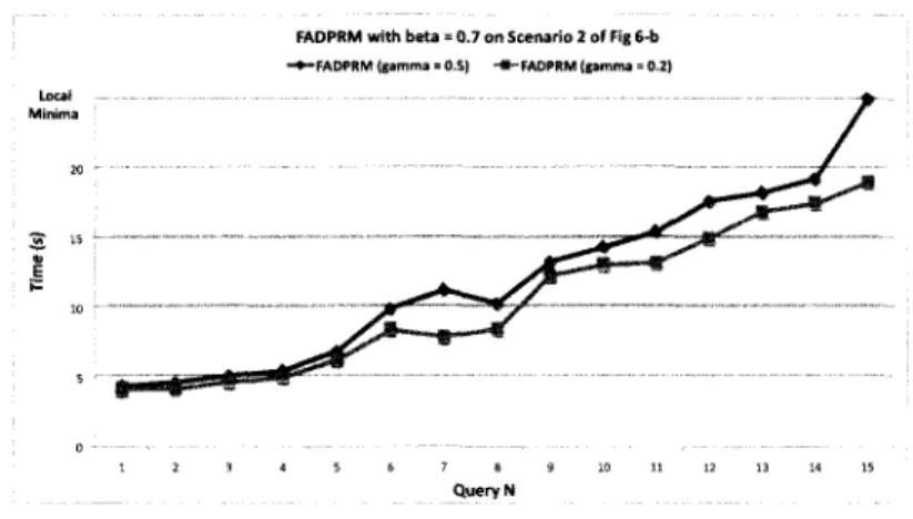
1.8 Path quality with FADPRM (/3 = 0,4 and {3 = 0, 7) 30 1.9 Planning time with FADPRM (0 = 0, 7) with 7 = 0, 5 and 7 = 0, 2 . . . . 31
1.10 Smoothed paths with FADPRM in the ISS environment ((3 = 0, 7) 32
1.11 FADPRM versus PRM in smoothing time 32 1.12 FADPRM versus PRM in path quality of smoothed paths 33
1.13 PUMA robot around a car 34 1.14 Path quality evolution with FADPRM 34
2.1 Roman tutor interface 41 2.2 Degrees of freedom of a virtual camera 42
2.3 Film abstraction hierarchy 43
2.4 ATDG architecture 48 2.5 Camera placements 51
TABLE DES M A T I E R E S
2.6 Examples of idioms 52 2.7 A shot composition rule 53 2.8 Shot specification operator 55 2.9 Idiom selection operator 56 2.10 Idiom-description LTL formula used to film a translation of the SSRMS . . 57
2.11 Idiom to film the SSRMS anchoring a new module on the ISS 58
2.12 Scenarios 59 2.13 Performance data 59
3.1 SSRMS on the ISS (left) and the robotic workstation (right) 65
3.2 Roman tutor interface 67 3.3 SSRMS going through three different cameras fields of view (purple, green
and blue cones) and avoiding an undesirable zone (rectangular zone in pale
red) 70 3.4 ATDG architecture 73
3.5 Idiom to film the SSRMS anchoring a new component on the ISS 74
3.6 Roman Tutor architecture 75 3.7 Roman Tutor showing a robot trajectory to the student 80
Introduction
La manipulation du bras robot canadien ou SSRMS (pour "Space Station Remote Ma-nipulator System") sur la station spatiale internationale (SSI) est une tache fortement com-plexe. Elle necessite la maitrise complete de la geometrie du robot et des differents modes de manipulation, ainsi qu'une connaissance approfondie de l'architecture de la station avec ses differents composants. La figure 1 montre une vue reelle de la SSI et du SSRMS. Le SSRMS est utilise pour deplacer une charge d'un endroit a un autre, reparer un des elements de la station et inspecter la station a l'aide d'une camera montee a son extremite. Toutes ces manipulations sont accomplies avec la plus grande precision de sorte que le SSRMS ne doit, en aucun cas, entrer en collision avec un element de la station.
figure 1 - SSRMS sur la station spatiale internationale
La manipulation du SSRMS se fait a distance, a partir d'un ordinateur situe a l'interieur d'un des compartiments de la SSI. Cet ordinateur comprend trois moniteurs relies chacun a une camera placee a un endroit particulier de la SSI. En tout, les cameras sont au nombre de quatorze, m o n i e s a differents endroits de la SSL Lors de la manipulation du SSRMS,
1.1. I N T R O D U C T I O N
un bon choix de cameras pour chacun des trois moniteurs s'impose. L'astronaute choisit celles qui lui offrent une meilleure visibility tout fen gardant une bonne appreciation de son evolution dans la tache. La difficulty de la manipulation du SSRMS provient surtout du fait que chacun des moniteurs ne presente qu'une vue partielle de la station. Nous utili-sons 1'appellation "manipulations robotisees" pour referer aux manipulations effectuees a distance par les astronautes a travers l'ordinateur pour deplacer le SSRMS.
Cette these a pour objectif de developper un systeme, dans notre cas un simulateur, tutoriel intelligent (STI) pour l'apprentissage de manipulations robotisees, applicable au SSRMS sur la SSL Le STI appele Roman Tutor (voir la figure 2), pour RObot MANipula-tion Tutor, est une preuve du concept de simulateur d'apprentissage autonome et continue pour des manipulations robotisees complexes. Un tel concept est pertinent pour les futures missions spatiales sur Mars ou sur la Lune. Meme si le SSRMS ne sera pas impliqu6 dans de telles missions a cause de sa trop grande complexity, le fait de demontrer qu'on peut concevoir un simulateur capable de donner des retroactions similaires a celles d'un ensei-gnant humain peut fournir des idees pour des concepts similaires applicables aux robots plus simples qui seront utilisees dans les prochaines missions sur Mars ou la Lune.
rktar OfftoJtyloml K d i M Tods About...
j-. ' st a w s
Action Applied 10 Result Cofllslon Details Proximity Detslls Movement W P (-180.SZ9444. -160.172366. 166.910689 J &
Movement W P [-180.<I69350,-160.023379, 166.904245] I Movement W P 1 - 1 8 0 . 4 0 7 1 1 1 . - l S 9 . S 7 S 2 f l 7 , 168.867^80) ^ Movement S P 1-188.107114.-1S9.87S217 . 1 6 8 . 8 6 7 1 8 0 ) : Mnvemcnt SV I-180.4074! 4 , -159.875247 , 168.867480) t
figure 2 - Roman tutor interface
1.1. INTRODUCTION
Roman Tutor constitue un outil de validation des operations robotisees utilisable par les equipes terrestres en support aux astronautes sur le SSI. En effet, la realisation d'une ope-ration impliquant le SSRMS sur le SSI necessite au prealable la validation par une equipe sur terre en liaison avec les astronautes. L'equipe sur terre utilise un simulateur du SSRMS pour valider les operations impliquant le SSRMS. Cependant, le simulateur actuel est es-sentiellement un outil de visualisation, sans aucune intelligence. II ne peut pas comparer differents scenarios possibles ni donner des retroactions pedagogiques aux operateurs (par exemple, expliquer pourquoi une manoeuvre est preferable a une autre). En fait, il revient aux operateurs de decider du deplacement du SSRMS dans le simulateur et comparer les differentes alternatives.
Contrairement a un simulateur normal, Roman Tutor a la capacite de comprendre, dans une certaine mesure, les manipulations du SSRMS pour pouvoir valider les manipulations faites par un operateur, les critiquer et suggerer de meilleures approches. Une des com-posantes permettant au STI cette capacite de comprendre les manipulations est un plani-ficateur des deplacements du SSRMS. Etant donne une configuration initiale du SSRMS et une configuration cible, le planificateur est en mesure de determiner une trajectoire me-nant de la configuration initiale a la configuration finale, teme-nant compte des obstacles et des contraintes de visibilite. Ainsi, etant donne une trajectoire faite par un operateur, Ro-man Tutor peut la critiquer par rapport a sa propre trajectoire et fournir des retroactions au besoin.
La planification de trajectoires pour des robots articules est un probleme fortement etudie en robotique et en intelligence artificielle, auquel plusieurs solutions ont ete propo-sees [36, 11, 22, 57, 44]. Dans sa forme classique, le probleme consiste a amener un robot d'une position a une autre en evitant la collision avec les obstacles presents dans le milieu. Une des choses qui rendent le probleme particulier dans Roman Tutor est son aspect for-tement dynamique resultant du fait qu'il doit suivre les deplacements du SSRMS effectues par un operateur pour les valider. Pendant que l'operateur deplace le SSRMS, le role du pla-nificateur est de verifier, a chaque mouvement, l'existence d'une trajectoire possible entre la configuration courante du robot et une configuration finale donnee comme cible a at-teindre. Roman Tutor ne peut pas prevoir a l'avance les mouvements de l'operateur; il doit recalculer dynamiquement la trajectoire vers la cible a partir de la configuration courante. Cela doit se faire efficacement en exploitant les calculs realises dans les etapes precedentes.
1.1. INTRODUCTION
Idealement, ceci necessite que le planificateur de trajectoire ait la propriete "anytime" [20], c'est-a-dire, qu'il soit capable de donner une solution approximative dans un delai limite; de sorte que plus le delai alloue est eleve, plus la solution est proche de l'optimalite.
Une autre particularite du probleme de planification de trajectoires dans Roman Tutor concerne les contraintes de visibilite. Le planificateur doit calculer des trajectoires visibles au travers des cameras montees sur la SSI et que l'operateur utilise pour voir l'exterieur de la SSI. Bien entendu, la contrainte de deplacer le SSRMS d'une position initiale vers une position finale en evitant les collisions demeure la contrainte la plus critique. II s'agit d'une contrainte dite dure parce que les collisions doivent etre evitees a tout prix. Par contre, dif-ferentes regions de la SSI peuvent etre plus ou moins visibles selon les cameras choisies et selon les conditions de l'environnement. Par exemple, l'orbite de la SSI peut faire en sorte qu'a differents moments des cameras deviennent exposees au soleil, rendant difficile la visibilite des regions couvertes par ces dernieres. Selon ce degre de visibilite, une tra-jectoire passant a travers certaines regions doit etre evitee le plus possible, mais peut etre
acceptee s'il s'avere impossible de trouver de meilleures solutions. Les contraintes de visi-bilite sont done des contraintes souples ou fiexibles. Elles expriment des preferences dans la navigation du robot.
Pour donner des retroactions, Roman Tutor utilise un generateur automatique de de-monstrations de taches ATDG pour "Automatic Task Demonstration Genrator". Etant donne la description d'une tache (par exemple, deplacer une charge d'un endroit a un autre), le ATDG genere une animation 3D interactive expliquant comment effectuer une telle tache. La conception du ATDG est inspiree des techniques de planification automatique des ani-mations 3D. Les techniques usuelles presentes dans la litterature sont de deux types : les approches par satisfaction de contraintes et les approches par idiomes (chapitre 2). Les ap-proches par satisfaction de contraintes travaillent au niveau de chaque image constituant le film et utilisent des methodes numeriques fastidieuses pour s'assurer de 1'exactitude et de la coherence de leur contenu. Les approches par idiomes s'inspirent du monde cinemato-graphique et utilisent differents concepts leurs permettant de filmer une animation comme le fait un metteur en scene. Vu le caractere tres complexe de notre application, les deux families d'approche s'averent etre inapplicables directement a notre problematique.
En resume, cette these a pour objectif le developpement d'un prototype simulateur tu-toriel intelligent pour l'apprentissage d'operations robotisees, appele Roman Tutor. Pour
1.1. INTRODUCTION
realiser ce prototype, nous nous proposons de developper et d'integrer trois composantes originales.
1. Un planificateur de trajectoires pour des environnements dynamiques presentant des contraintes dures et flexibles.
2. Un generateur automatique de demonstrations de taches (ATDG). Ce dernier fait appel au planificateur de trajectoires pour trouver une trajectoire solution a une tache de deplacement du SSRMS et a des techniques de planification des animations pour filmer la solution obtenue.
3. Un modele pedagogique implementant des strategies d'intervention pour donner de l'aide a un operateur manipulant le SSRMS.
Le premier chapitre de cette these introduit la nouvelle approche de planification de trajectoires avec preferences que nous avons developpee. Cette nouvelle approche etend les approches de planification de trajectoires par echantillonnage actuelles par l'ajout de la caracteristique flexible permettant de tenir compte des contraintes souples dans l'envi-ronnement, et de la tenir compte des contraintes de visibilite sur la SSI. Les approches par echantillonnage sont les plus efficaces dans des environnements a forte complexity [30]. Nous montrons dans ce chapitre que cette notion de flexibility permet d'ameliorer grande-ment la qualite des trajectoires generees, un des plus importants handicaps des approches par echantillonnage. De plus, ce nouveau planificateur adapte les caracteristiques "anyti-me" et dynamique au sein des approches de planification par echantillonnage.
Le deuxieme chapitre est consacre a l'etude de l'ATDG, le generateur automatique de demonstrations de taches. ATDG utilise la logique temporelle lineaire (LTL) [3] pour ex-primer les principes cinematographiques et les preferences de filmage, un langage plus expressif et avec une semantique plus simple que les anciens langages de planification de cameras. ATDG implemente l'algorithme sous-jacent TLPlan pour la planification de cameras. Tout d'abord, la trajectoire du robot est generee en utilisant le planificateur de tra-jectoires. Le planificateur de cameras TLPlan est ensuite invoque pour trouver la meilleure
sequence de configurations de cameras filmant le robot sur sa trajectoire.
Dans le troisieme et dernier chapitre de cette these, nous exposons le modele pedago-gique implemente au sein de Roman Tutor pour supporter et encadrer l'apprentissage de manipulations robotisees. L'aide a un operateur fait appel d'une part a des demonstrations
1.1. I N T R O D U C T I O N
de taches generees automatiquement par le ATDG, et d'autre part au planificateur de tra-jectoires pour suivre la progression de l'operateur sur sa tache, lui fournir de l'aide et le
Chapitre 1
Planification de trajectoires avec
preferences dans des environnements
dynamiques tres complexes
Resume
Les approches de planification de trajectoires presentes dans la litterature peuvent etre classees en deux principales categories : les approches combinatoires et les approches par echantillonnage [14, 44], Les approches par echantillonnage ou PRMs (pour "Probabilistic Roadmap Methods") sont les plus efficaces dans des environnements a forte complexite [30]. Leur caracteristique probabiliste leur permet d'eviter la representation explicite et complete de l'espace. Par echan-tillonnage probabiliste, elles construisent un roadmap ou graphe qui n'en est qu'une representation simplifiee. Vu la complexite accrue des environnements dans lesquels oeuvrent les robots propres a notre problematique, il semble evident que la nouvelle approche de planification de trajectoires que nous presentons dans ce chapitre soit alignee a cette categorie de planificateurs.
Dans sa formulation traditionnelle, le probleme de planification de trajec-toires consiste a amener un robot d'une position a une autre en evitant la col-lision avec les obstacles presents dans l'environnement. Dans certaines applica-tions complexes du monde reel, toutefois, en plus des obstacles qui doivent etre
evites, il peut y avoir des zones dangereuses qui doivent etre evitees autant que possible. La notion de danger est pertinente par exemple dans des applications militaires [51, 59], Inversement, il peut etre souhaitable pour un chemin de rester a proximite de certaines zones autant que possible. C'est notamment le cas dans la manipulation du SSRMS sur la SSI, ou les preferences sont liees a des champs de visions de cameras, qui changent de fagon dynamique, en partie a cause des changements dans l'orbite de la SSL
Nous presentons dans les pages qui suivent un article qui introduit notre nou-velle approche de planification de trajectoires avec preferences. Cette nounou-velle approche est intitulee FADPRM pour "Flexible Anytime Dynamic PRM". Le pla-nificateur FADPRM va etendre les approches de planification PRMs actuelles par l'ajout de la caracteristique flexible permettant de tenir compte des contraintes souples dans l'environnement. Les contraintes souples (ou flexibles) sont dictees par la presence de zones avec differents degres de desirabilite dans l'environ-nement. FADPRM previlegie des trajectoires solutions qui evitent les zones non desirables et qui font passer le robot le plus possible a travers les zones desirables. Meme quand un probleme de planification de trajectoires ne necessite pas l'ajout de la notion de desirabilite de maniere explicite, l'introduire permet de fournir un moyen efficace pour controler la qualite des trajectoires generees par une methode de planification par echatillonnage. En effet, dans les approches par echantillonnage, les trajectoires sont obtenues en reliant des configurations qui sont choisies au hasard dans l'espace des configurations libres. Ceci conduit a des trajectoires solutions complexes et de mauvaise qualite, necessitant de operations heuristiques de post-traitement pour les lisser [58]. Dans l'article suivant, nous demontrons qu'il est possible d'influencer la strategie d'echantillonnage pour generer des trajectoires plus lisses juste en specifiant des zones avec degres de desirabilite dans l'environnement. Nous montrons egalement que la notion de desirabilite permet un meilleur controle de 1'exploration de l'espace de recherche pour garantir une planification plus efficace.
Avec FADPRM, l'exploration par echantillonnge de l'espace des configura-tions libres s'inspire de differentes strategies d'exploration dynamiques et "any-time" presentes dans le litterature [47, 48, 39]. Un planificateur de trajectoires
peut s'adapter aux changements dynamiques qui surviennent dans l'environne-ment (changel'environne-ment dans les obstacles, dans les zones et dans leurs degres de de-sirabilite ou dans les configurations initiale et finale) en recalculant une nouvelle trajectoire a chaque fois. Une strategic dynamique reutilise les resultats obte-nus des recherches anterieures pour garantir de meilleures performances dans la planification. Une strategic "anytime" [20] procede de maniere incremental, en commen§ant par un plan de degre de desirabilite bas, puis l'ameliore progressi-vement. De cette fa§on, et a tout moment, le planificateur dispose d'un plan d'un certain degre de satisfaction qui est ameliore si plus de temps de planification est disponible.
Commentaires
Une premiere version du planificateur FADPRM a ete presentee a la conference "IEEE International Conference on Robotics and Automation" en 2006 [7]. Dans cette derniere, FADPRM utilisait la strategie d'exploration AD* pour "Anytime Dynamic A*" [48]. Dans sa nouvelle version presentee dans les pages qui suivent, FADPRM implemente une version "anytime" de la strategie plus recente GAA* pour "Genralized Adaptive A*" [61]. Nous utilisons maintenant GAA* a la place de AD* parce que les deux algorithmes ont des performances comparables et que GAA* a une structure plus simple et plus facile a comprendre et a implementer.
L'article presente dans ce chapitre a ete soumis au journal "International Journal of Robotics Research". Une version plus courte de ce travail va pa-raitre dans les actes de "International Conference on Autonomous and Intelligent Systems" [6]. Dans la version courte, seulement 1'adaptation du planificateur GAA* dans FADPRM sans integrer de la strategie "anytime" a ete presentee. Ces travaux ont ete realises, valides et rediges sous la supervision du Professeur Froduald Kabanza (Universite de Sherbrooke) et avec les conseils du Professeur Leo Hartman (Agence spatiale canadienne).
Randomized Path Planning with Preferences
in Highly Complex Dynamic Environments
Khaled Belghith, Froduald Kabanza
Departement d'informatique, Universite de Sherbrooke, Sherbrooke, Quebec, Canada J1K 2R1
[email protected], [email protected]
Leo Hartman
Canadian Space Agency,
John H. Chapman Space Centre, 6767 Route de l'Aeroport Saint-Hubert, Quebec J3Y 8Y9
leo.hartman®asc-csa.gc.ca
Abstract
In this paper, we consider the problem of planning paths for articulated bo-dies operating in workplaces containing obstacles and regions with preferences expressed as degrees of desirability. Degrees of desirability could specify dan-ger zones and desire zones. A planned path should not collide with the obstacles and should maximize the degrees of desirability. Region desirability can also convey search-control strategies guiding the exploration of the search space. To handle desirability specifications, we introduce the notion of flexible probabilis-tic roadmap (flexible PRM) as an extension of the traditional PRM. Each edge in a flexible PRM is assigned a desirability degree. We show that flexible PRM planning can be achieved very efficiently with a simple sampling strategy of the configuration space defined as a trade-off between a traditional sampling oriented towards coverage of the configuration space and a heuristic optimization of the path desirability degree. For path planning problems in dynamic environments, where obstacles and region desirability can change in real-time, we use dynamic and anytime search exploration strategies. The dynamic strategy allows the plan-ner to re-plan efficiently by exploiting results from previous planning phases. The anytime strategy starts with a quickly computed path with a potentially low desi-rability degree which is then incrementally improved depending on the available planning time.
1 . 1 . INTRODUCTION
1.1 Introduction
In its traditional form, the path planning problem is to plan a path for a moving body (ty-pically a robot) from a given start configuration to a given goal configuration in a workspace containing a set of obstacles. The basic constraint on solution paths is to avoid collision with obstacles, which we call hereby a hard constraint. There exist numerous approaches for path planning under this constraint [36, 11, 22, 57, 44].
In many complex applications, however, in addition to obstacles that must be avoided, we may have dangerous areas that must be avoided as much as possible. That is, a path going through these areas is not highly desirable, but would be acceptable if no better path exists or can be computed efficiently. The danger concept is relevant, for example, in mi-litary applications. Some path planning techniques that deal with it have been proposed, including [59, 51]. Conversely, it may be desirable for a path to stay close to certain areas as much as possible. Even when a path planning problem has no explicit notion of region desirability, introducing the notion provides a way to control the quality of a path generated by a randomized path planning method. Indeed, paths are obtained by connecting miles-tones that are randomly sampled in the free workspace and this tends to yield awkward paths, requiring heuristic post-processing operations to smooth them. In this paper, we de-monstrate that one can influence the sampling strategy to generate less awkward paths by specifying zones the path is preferred to go through. We also show that region desirability specifications can also help control the exploration of the sampled search space and make the path-planner more efficient.
Our path planning approach builds flexible roadmaps by extending existing sampling techniques including delayed collision checking, single query, bi-direction and adaptive sampling [58]. Desirable and undesirable workspace regions are soft constraints on the robot path, whereas obstacles are hard constraints. The soft constraints convey preferences for rating solutions paths which must avoid obstacles. The more a path avoids undesirable zones and goes through desirable zones, the better it is.
The exploration of the sampled configuration space is done using dynamic and anytime space exploration methods [47,48, 39]. In dynamic environments, a path planner can adapt a previously computed path to dynamic changes in obstacle configurations, goals or region desirability, by computing a new path. Dynamic state space exploration strategies reuse
1 . 1 . I N T R O D U C T I O N
the results obtained from previous searches to achieve better performance compared to re-searching from scratch. In addition, an anytime search strategy proceeds incrementally, starting with a path having a low desirability degree and then improving it incrementally. In this way at "any time", the planner has a plan with some degree of satisfaction that is improved as more planning time is spent.
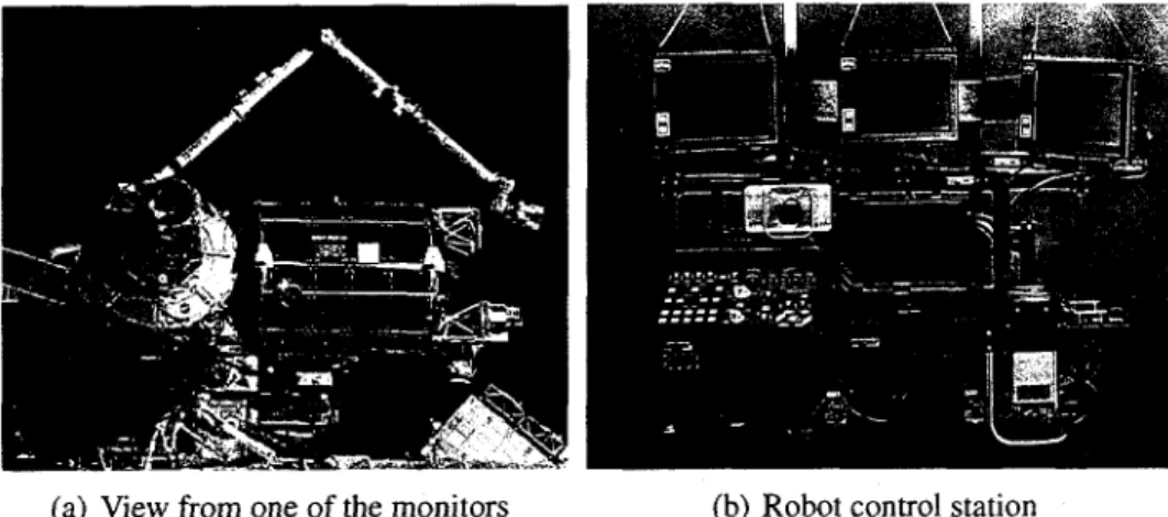
Our testbed is a simulation of the Space Station Remote Manipulator System (SSRMS) deployed on the International Space Station (ISS). The SSRMS is a 17 meter long arti-culated robot manipulator, having a translation joint, seven rotational joints (each with a range of 270 degrees) and two latching end-effectors which can be moved to various fix-tures, giving it the capability to "walk" from one grappling fixture to next on the exterior of the ISS [19]. Astronauts operate SSRMS using the robot control station located inside one of the ISS compartments (Figure 1.1). A robot control station has an interface with three monitors, each connected to a camera placed at a strategic location of the ISS. There are many cameras covering different parts of the ISS structure and three of them are selected and mapped to the three monitors.
(a) View from one of the monitors (b) Robot control station
figure 1.1 - ISS path-planning domain and robot control station
Most of the SSRMS tasks on the ISS involve moving the robot from one configuration to another in order, for example, to move a payload from the shuttle or inspect a region of the ISS exterior using a camera mounted on the end effector. A judicious choice of the camera on each of the three monitors along different segments of a robot path ensures that the operator is appropriately aware of the robot motion. Computed paths must go as
1 . 2 . B A C K G R O U N D AND R E L A T E D W O R K
much as possible through camera fields of view to enable a good appreciation of the robot motion. In other words, the camera fields of view convey preferences for regions through which the robot path should remain as much as possible while avoiding collisions with the ISS structure.
In the next section we give the background and discuss some of the related work. We then present our path planning approach to handling path preferences in the robot works-pace. We follow with experiments in the ISS environment and in a car repair domain, showing the capability of the new planning approach to handle path preferences and search control specifications that are expressed by assigning desirability degrees to workspace regions.
1.2 Background and Related Work
A configuration q of an articulated robot with n degrees of freedom ( d o f ) is an n ele-ment vector of the robot joint positions. Since the robot moves by changing its joint rota-tions or translarota-tions, a path between two points is a sequence of configurarota-tions sufficiently close together connecting the two points. A path is free or in the space of collision-free configurations C /r e e, if the robot does not collide with any obstacle in the workspace in any of the configurations on the path. Computing a path is seen as making a query (to the path-planner) with the input of the start and goal configurations. Two very commonly used approaches to path planning are the combinatorial and randomized approaches.
Combinatorial approaches, also called decomposition or exact approaches, proceed by searching through a geometric representation of C /r e e. Given a 2D or 3D model of obstacles in the workspace, a 2D or 3D model of the robot, the configuration space is decomposed into an occupancy grid of cells, also called a roadmap. A path from a start cell to a goal cell is then found by searching a sequence of moves between adjacent free cells, connecting the start configuration to the goal [38, 49, 22, 44]. These moves correspond to possible edges in a graph with nodes corresponding to free cells in the grid. Graph-search algorithms such as A* search [29, 54] or AD* [48] can be used to compute a path between the start and goal configurations.
Randomized approaches, also known as sampling-based approaches, proceed by sam-pling the space of the robot configurations. Given a 2D or 3D model of obstacles in the
1 . 2 . BACKGROUND AND R E L A T E D W O R K
workspace and a 2D or 3D model of the robot, a randomized planner builds a graph of nodes corresponding to configurations in Cfree by picking configurations randomly and checking
that they are collision-free. It uses a fast collision detection checker (called a local planner) to check that an edge between two adjacent nodes is also collision-free; each time the lo-cal planner succeeds, the corresponding edge (i.e., lolo-cal path or path segment) is inserted into the graph. The graph built that way is called a probabilistic roadmap (PRM) [36] or a rapidly-exploring random tree (RRT) [44] and is a simplified representation of C /r e e. Here too graph-search algorithms such as A* search [54] or AD* [48] can be used to explore the graph to find a collision-free path linking the start to the goal configuration.
Therefore combinatorial as well as randomized approaches have in common the discre-tization problem to build an intermediate graph structure (the roadmap) and search through it. The key difference lies in what the graph represents and how it is built. With combinato-rial approaches the graph is meant to be an exact representation of Cfree and its construction
takes into account the geometry of the workspace and the robot. With sampling approaches, the graph represents samples of Cfree. It is not an exact representation of C /r e e. Given that the configuration space is randomly sampled, randomized approaches do not guarantee a full coverage of free space and they are not complete and do not guarantee optimality. In fact, they are probabilistically complete, meaning that the more samples are made the closer the probability of guaranteeing the absence or presence of a solution gets to 1 [58]. Com-binatorial approaches guarantee completeness and optimality by using a sufficiently small discritization step. In practice, this results in large search spaces, making the approaches generally intractable for high dimensional configuration spaces [30].
A heuristic method for grid decompositions is to plan using a coarse discretization space. If no solution is found or to improve the solution found so far, a new planning ite-ration is made with finer discretization pace. The process can be iterated as more planning time is invested or until a satisfactory solution is found. Another exploration strategy for the occupancy grid maybe to use random search [45], While this may help coping with the complexity of the configuration space, in very large configuration spaces the planner spends a large amount of time generating the occupancy grid [30]. Sampling-based methods ge-nerally offer better performance than exact methods for domains with high-dimensional spaces [30, 14, 44],
1 . 2 . B A C K G R O U N D A N D R E L A T E D W O R K
1.2.1 Probabilistic Roadmap Approach
Our randomized implementation follows a PRM approach [58], However, it can be easily adapted to an RRT approach given an RRT approach fundamentally corresponds to a single-query PRM with on the fly search of the sampled roadmap combined with on-the-fly collision detection [45]. Our implementation includes various configuration modes that allow the planner to run in a single or multiple query mode, with on-the-fly search of the roadmap or not and with collision detection on-the-fly or delayed.
A PRM is an undirected graph G = (N, V) with N the nodes of the graph and V the arcs. The nodes are sampled configurations in C/r e e, also called milestones. The arcs represent links or segments v connecting two configurations. Algorithm 1 shows a basic PRM path planning algorithm. It starts by initializing the roadmap G with the start and goal configurations nstart and ngoai. Then, a new node n is sampled randomly, with a probability
measure 7r, in Cfree and added to the roadmap. A set of nodes in G and in the neighborhood
of n called Vn is selected. Using a collision checker (local planner), we look for a node n'
in Vn such that the link (n, n') is free of collisions and then add it to G. The process is
repeated until a path connecting nstart and ngoai is found. Algorithm 1 Basic PRM Algorithm
01. Initialize the roadmap G with two nodes, nstart and ngoai 02. Repeat
03. Sample a configuration n from Cfree with probability measure IT
04. if (n e Cfree) then add n as a new node of G
05. for some nodes n' in a neighborhood Vn of n in G such that n' / n
06. if collisionFree(n, n') then add v = (n, n') as a new edge of G
07. until nSTART a nd rig0aL are in the same connected component of G or G contains N + 2 nodes
08. if fistart^nd ngoai are in the same connected component of G then
09. return a path between them
10. else
11. return No Path
The above algorithm follows a single-query on-the-fly collision detection approach. The samples of Cfree corresponding to the nodes in the graph G are generated while
sear-ching G and detecting collision on the fly. On each query, the graph is reconstructed. It is conceivable to generate G, store it and then search it each time we have a query. In this case, a sufficiently large G needs to be generated to cover potential queries. This is known as a multiple-query approach because several queries can be made on the same roadmap. A
1 . 2 . B A C K G R O U N D AND R E L A T E D W O R K
delayed collision-checking approach would avoid checking collisions (Step 6) until a whole path has been found. If a segment on the path turns out to be colliding, the algorithm would backtrack to search for a new path. A delayed collision-checking method can outperform a non-delayed one on some planning domains [11, 58].
A PRM planner selects a node to expand in the free configuration space according to some given sampling measure. The efficiency of PRM approaches significantly depends on this measure [30], A naive sampling measure will likely lose efficiency when the free space
Cfree contains narrow passages. A narrow passage is a small region in Cfree where the
sampling probability becomes very low. Some approaches exploit the geometry of obstacles in the workspace to adapt the sampling measure accordingly [9, 40, 41]. Other methods use machine learning techniques to adapt the sampling strategy dynamically during the construction of the probabilistic roadmap [41, 13, 31].
1.2.2 Path Planning with Preferences
In addition to collision avoidance, the concept of dangerous areas that have to be avoi-ded as much as possible has been addressed in some path planning approaches [51, 59]. Herein we generalize the concept to preferences among regions in the Cfree space.
Dif-ferent regions can be assigned difDif-ferent degrees of desirability, meaning that we would like the path planner to compute a path which not only avoids obstacles but also maximizes the degree of desirability for the path. Since path quality criterion may also depend on other metrics such as the distance along the path, we define the overall path quality as a trade-off between region desirability and distance. The trade-off is conveyed by a parame-ter weighing the contribution of each of these criparame-teria to the global path-quality criparame-terion. As a means to convey preferences among collision-free paths, region desirability provides a way to specify search control information for a path planner. It can be used to determine how the search process chooses the next node to expand.
1.2.3 Anytime Path Planning
In real-time applications involving the computation of an optimal solution, it is often desirable to have an incremental algorithm that computes its solution as a sequence of in-termediate useful, but suboptimal solutions, converging towards an optimal solution. Dean
1 . 2 . B A C K G R O U N D AND RELATED W O R K
and Boddy called these anytime algorithms [20]. Such an algorithm guarantees a useful ap-proximate solution at any time, which gets improved incrementally if more planning time is allowed. With a PRM planner, an anytime capability can be integrated into the search al-gorithm exploring the sampled roadmap. In particular, using the A* heuristic graph-search algorithm, one can implement a twofold anytime capability.
If given a transition function covering the entire search space and an admissible heuris-tic, A* guarantees finding an optimal solution. In our case, the search space is the sampled roadmap and a heuristic function h{n) is a function taking a configuration n as input and returning the estimated distance from a configuration n to the goal configuration. It is ad-missible if it never overestimates the actual distance h*{n). We use the Euclidean distance as admissible heuristic. Obviously, the larger the search space, the more time it may take to find an optimal solution, even though A* does not have to exhaust the search space to guarantee optimality. To mitigate the combinatorial size of the state space, one can run A* on a smaller portion of the search space (producing an approximate path), then expand the search space and compute a new solution path for it and so on. This gives a sequence of solutions, converging to the optimal when the entire search space is covered. Given a dead-line for computing a solution, the search space will be iteratively expanded accordingly ; a solution for each chunk of expansion is then computed. This implements an anytime capa-bility through state expansion. The search process can be stopped at any time and give a solution (more precisely anytime after the time necessary for a first solution) and the more time it is given, the better the solution will be.
Another interesting property of A* is that, if given a non admissible heuristic h(n) =
h*(n) + e, then the cost of the path computed by A* minus the cost of the optimal distance
is less or equal than e. In other words, e is an upper bound on the error for the cost of the solution compared to the optimal solution. Moreover, A* tends to return a solution, possibly suboptimal, faster with inadmissible heuristics than with admissible heuristics. Based on these two observations and given an admissible heuristic h (e.g., the Euclidean distance), another way to implement an anytime A* search would be to compute a path using h{n) + ei, then another solution using h(n) + e2 and so on. In other words, a sequence of solutions using a decreasing error bound Q on the admissible heuristic is computed, with ei +i < €j. Given a deadline for computing a solution path, the inflating factor will be decreased iteratively, computing a solution for each decrease. This is the anytime capability
1 . 3 . F A D P R M PATH P L A N N E R
through heuristic improvement.
Both previous methods for implementing anytime capabilities with A* are comple-mentary and can be combined as is the case in the Anytime Repairing A* (ARA*) algo-rithm [49]. We use a similar approach to explore a randomized flexible roadmap.
1.2.4 Dynamic Path Planning
In the ISS environment, most of the structure is fixed, only the robots can move. Ho-wever, region desirability degrees can change as well as the goal. Regions of desirability depend on the task and the involved camera views. Depending on the orbit of the ISS, a camera may have its view towards the sun, making it undesirable. From the roadmap pers-pective, this means that the cost of a segment between two nodes can change dynamically. Such changes may invalidate a previously calculated path, either because it is no longer optimal or simply because it now leads to a dead-end. Re-planning is necessary in such cases.
Dynamic path planners adapt dynamically to change happening around the robot by repairing incrementally their representation of the environment. Different approaches exist that are extensions of the A* algorithm, including D* Lite [38], Anytime Dynamic A* (AD*) [48] and Generalized Adaptive A* (GAA*) [61]. These algorithms extends A* search to solve dynamic search problems faster by updating heuristics on nodes using knowledge acquired from previous searches.
1.3 FADPRM Path Planner
Combining region preferences, anytime search and dynamic re-planning, we obtain a flexible anytime dynamic probabilistic roadmap planner (FADPRM). The general idea is to keep track of milestones in an optimal solution to the goal. When changes are noticed, edges costs are updated and a new roadmap is re-computed fast, starting from the goal, taking into account previous traces of the path-calculation. This brings us back to a method in between the multiple query approach and the single query approach. The difference with a multiple query approach is that we are now only concerned with the roadmap to the current goal the robot is trying to reach in a dynamic environment.
1 . 3 . F A D P R M PATH P L A N N E R
FADPRM uses GAA* to explore the roadmap. The cost of an edge between two confi-gurations depends on the actual distance between the conficonfi-gurations and the desirability degrees of the configurations along that edge. In a preliminary version of FADPRM [7], we have used AD* instead of GAA*. We now use GAA* instead of AD* because they have comparable performances, yet GAA* has a simpler description. Note that the contri-bution of FADPRM does not just amount to using GAA* to explore a sampled roadmap. The integration of preferences and their use to control both the path quality as well as the search-process for computing such a path are the key contributions.
1.3.1 Algorithm Sketch
FADPRM works with Cfree segmented into zones, each zone being assigned a degree
of desirability (dd), that is, a real number in the interval [0 1], The closer is dd to 1, the more desirable the zone is. Every configuration in the roadmap is assigned a dd equal to the average of dd of zones overlapping with it. The dd of a path is an average of dd of configurations in the path. An optimal path is one having the highest dd.
The input for FADPRM is thus : a start configuration, a goal configuration, a 3D model of obstacles in the workspace, a 3D specification of zones with corresponding dd and a 3D model of the robot. Given this input:
1. To find a path connecting the input and goal configuration, we search backward from the goal towards the start (current) robot configuration. Backward instead of forward search is done because the robot moves; we want to re-compute a path to the same goal but from the current position whenever the environment changes before the goal is reached.
2. A probabilistic priority queue OPEN contains nodes on the frontier of the current roadmap (i.e., nodes that need to be expanded because they have no predecessor yet; or nodes that have been previously expanded but are not being updated anymore) and a list CLOSED contains non frontier nodes (i.e., nodes already expanded)
3. Search consists of repeatedly picking a node from OPEN, generating its predeces-sors and putting the new ones and the ones not yet updated in OPEN.
(a) Every node n in OPEN has a key priority proportional to the node's density and best estimate to the goal. The density of a node n, density(n), reflects the
1 . 3 . F A D P R M PATH P L A N N E R
density of nodes around n and is the number of nodes in the roadmap with confi-gurations that are a short distance away. The estimate to the goal, f(n), takes into account the node's dd and the Euclidean distance to the goal configuration as explained below. Nodes in OPEN are selected for expansion in decreasing priority. With these definitions, a node n in OPEN is selected for expansion with priority proportional to
(1 — (3) / density in) + /3 * fin),
(3 is the inflation factor with 0 < [3 < 1.
(b) To increase the resolution of the roadmap, a new predecessor is randomly gene-rated within a short neighborhood radius (the radius is fixed empirically based on the density of obstacles in the workspace) and added to the list of prede-cessors in the roadmap generated so far; then the entire list of predeprede-cessors is returned.
(c) Collision is delayed : detection of collisions on the edges between the current node and its predecessors is delayed until a candidate solution is found; if col-liding, we backtrack and rearrange the roadmap by eliminating nodes involved in this collision.
4. The robot may start executing the first path found. 5. Concurrently, the path continues to be improved.
6. Changes in the environment (moving obstacles and zones or changes in dd for zones) cause updating of the roadmap and replanning.
With f3 equal to 0, the selection of a node to expand is totally blind to zone degrees of desirability and to edges costs (Euclidian distance). Assuming OPEN is the entire road-map, this case corresponds to a normal PRM and the algorithm probabilistically converges towards an optimal solution as is the case for a normal PRM [58]. With (3 = 1, the selection of a node is a best-first strategy and by adopting an A*-like f(n) implementation, we can guarantee finding an optimal solution within the resolution of the roadmap sampled so far. Therefore the expression (1 — (3)/density(n) + f3 * f(n) implements a balance between fast-solution search and best-solution search by choosing different values for (3.
1 . 3 . F A D P R M PATH P L A N N E R
Values of /3 closer to 1 give better solutions, but take more time. An initial path is generated fast assuming a value close to 0, then (3 is increased by a small quantity, a new path is computed again and so on. At each step, we have a higher probability of getting a better path (probability 1 when /3 reaches 1). This is the key in the anytime capability of our algorithm.
The heuristic estimate is separated into two components g(n) (the quality of the best path so far from n to the goal configuration) and h(n) (estimate of the quality of the path from n to the start configuration), that is, f(n) = (g(n) + h(n))/2; we divide by 2 to normalize f{n) to values between [0,1]. This definition of f(n) is as in normal A* except that:
- We do backward search, hence g(n) and h(n) are reversed.
- The quality of a path is a combination of its dd and its cost in terms of distance traveled by the robot. Given pathC ost(n, n'), the cost between two nodes, g(n) is defined as follows :
g(n) = pathdd(ngoah n)/{ 1 + 7pathC ost{ngoah n))
with 0 < 7 < 1.
- The heuristic h(n) is expressed in the same way as g(n) and estimates the cost of the path remaining to reach nstart :
h(n) = pathdd(n, nstart)/(1 + 7pathCost(n, nstart))
The factor 7 determines the influence of the dd on g(n) and on h(n). With 7 = 0, nodes with high dd are privileged, whereas with 7 = 1 and with the dd of all nodes equal to 1, nodes with least cost to the goal are privileged. In the last case, if the cost between two nodes pathCost(n,n')) is chosen to be the Euclidean distance, then we have an admis-sible heuristic and the algorithm is guaranteed to converge to the optimal solution. When
dd's are involved and since zones can have arbitrary configurations, it is difficult to define
admissible heuristics. The algorithm guarantees improvement of the solution, but it's im-possible to verify optimality. Since the dd measures the quality of the path, the idea is to run the algorithm until a satisfactory dd is reached. The functions pathdd and pathCost are implemented by attaching these values to nodes and updating them on every expansion or when dynamic changes are observed in the environment.
1 . 3 . F A D P R M PATH P L A N N E R
1.3.2 Algorithm Details
The detailed structure of the FADPRM path planner is presented in Algorithm 2. Since FADPRM proceeds backwards, it updates h-values with respect to the start configuration of all expanded nodes n after every search as follows :
h(n) = g(n8tart) ~ g{n).
Following GAA*, FADPRM does not initialize all g-values and h-values up front. Instead, it uses the variables counter, search(n) and pathcost(x) to decide when to initialize and update them by calling UpdateState() :
- The value of counter is x in the .xth execution of ComputeOrlmprovePath, that is, the xth call for GAA* on the roadmap.
- search(n) stores the number of the last search that generated node n. FADPRM
initializes these values to 0 for new nodes in the roadmap.
- pathcost(x) stores the cost for the best path found on the roadmap by the xth search.
More precisely, the formula for pathcost(x) is :
pathcost(x) =g(nstart) = pathdd(ngoahnstart) / (1 + 7 pathCost(ngoahnstart))
Nodes in OPEN are expanded in decreasing priority to update their g-values and their predecessors' g and h-values. The ordering of nodes in OPEN is based on a node priority
key(n), which is a pair [ki(n), k2(n)] defined as follows :
key(n) = [(1 — (3) / density (n) + (3f(n), h(n)],
with f(n) = [(g(n) + h(n)]/2 and key(n) < key[n!) if ki(n) < ki(n') or {k\{n) = ki(n') and k2(n) < k2(n')). During the update on nodes, FADPRM initializes the g-value of nodes
not yet generated by an already performed search, nodes with search(n) = 0, to zero. In the function ComputeorlmprovePathQ, when a node n with maximum key is extracted from OPEN, we first try to connect it to nstart using a fast local planner as in
SBL [58]. If it succeeds, a path is then returned (line 16). The expansion on a node n with maximum key from the OPEN (line 18) consists of sampling a new collision-free node in the neighborhood of n [58] and then the sampled node is added in the set Pred{n). After increasing the connectivity of the roadmap by adding a new node, FADPRM executes an
1 . 3 . F A D P R M PATH P L A N N E R
Algorithm 2 FADPRM Algorithm
01. KEY(N) 33. while (Not collision-free Path)
02. f(n) = [g(n) + h(n)]/2; 34. Rearrange T r e e ; 03. return [(1 - 0)/density (n) + /3.f(n);h(n)]\ 35.
36.
ComputeorlmprovePathQ;
counter = counter + 1;
04. UPDATES TATE (TI) 37. if (OPEN = 0)
05. if ((search(n) ^ 0) AND (search(n) ^ counter)) 38. pathcost(search(n)) = 0; 06. if (<?(n) + h(n) < pathcost(search(n)) 39. e l s e
07. h(n) = pathcost(search{n)) — g{n)\ 40. pathcost(search(n)) = g(nstart); 08. g(n) = 0; 41. publish current 0o—suboptimal solution ;
09. e l s e if (search(n) = 0) 42. while (nstart not in neighborhood of ngoai)
10. g(n) = 0; 43. if ("start changed)
11. search(n) = counter; 44.
45.
if (addtoTree(nst0rt))
publish current solution;
12. COMPUTEORIMPROVEPATH() 46. if changes in edge costs are detected
13. w h i l e (NoPathfound) 47. for all changed edges (u, v)
14. remove n with max key f r o m OPEN : 48. Update the edge cost c(u, v):
15. if (Connect(n, nstart)) 49. U p d a t e S t a t e ( u ) ;
16. r e t u r n /3-suboptimal p a t h ; 50. Update the priorities for all
17. else 51. n € OPEN according to Key(n);
18. ExpandNode(n);
For all n' 6 Pred(n)
52. CONSISTENCYPROCEDURE() ;
19.
ExpandNode(n);
For all n' 6 Pred(n) 53. decrease 0 or replan f r o m scratch ;
20. UPDATESTATE(H'); 9(«') = g(n) + c(n,n')-54. if ( 0 < 1) 21. UPDATESTATE(H'); 9(«') = g(n) + c(n,n')- 55. increase /3;
22. insert n' into OPEN ; 56. CLOSED = 0;
23. insert n into CLOSED ; 57.
58.
while (Not collision-free Path) Rearrange T r e e ;
24. MAINQ 59. C o m p u t e o r l m p r o v e P a t h Q ;
25. counter = 1; 60. counter — counter + 1;
26. g(nstart) = g(ngoal) = 0; 61. if (OPEN = 0)
27. sear ch(n start) = search(ngoai) = 0; 62. pathcost(search(n)) = 0;
28. /3 = A>; 63. else
29. OPEN = CLOSED = 0 ; 64. pathcost(search(n)) = g(nstart);
30. UPDATESTATE(NSTART) : 65. publish current j3—suboptimal solution;
31. UPDATESTATE(NGOOI) ; 66. if (/? = 1)
32. insert ngoal into OPEN with key{ngoai); 67. wait for changes in edges c o s t ;
update of the heuristics of all nodes in Pred(n) in order to make them more informed and then allow for later more focused searches.
FADPRM updates the h-values of node n (line 7) if different conditions are satisfied : - The node has not yet been generated by the current search ( s e a r c h ( n ) ^ counter) - The node was generated by a previous search (search(n) ^ 0)
- The node was expanded by the search that generated it last
(g(n) + h(n) < path.cost(counter))
FADPRM sets h(n) (line 7) to the difference between g{nstart) that is the cost of the path
from nstart to ngoai during the last search that expanded n and g(n) that remained the same
since the same search. Dynamic changes in the environment affect (increase or decrease) edge costs. Such changes are handled by a consistency procedure, adapted from GAA*
1 . 4 . E X P E R I M E N T A L R E S U L T S
and described in Algorithm 3. This procedure invoked at line 52 of the main algorithm whenever a cost decrease is observed. When invoked, it updates the h-values with respect to the start node.
Algorithm 3 Consistency Procedure
01. CONSISTENCYPROCEDUREQ
02. update the increased and decreased action costs (if a n y ) ; 03. OPEN = 0 ;
04. for all edges ( n , n')
05. with (n ^ nstart) and edge cost c,(s, s') decreased
06. UPDATESTATE(H); 07. UPDATESTATE(N'); 08. if O(n) > c(n,n') + h(n')) 09. h(n) = c(n,n') + h(n') 10. if neOPEN 11. delete n f r o m OPEN ;
12. insert n in OPEN with key-value KEY(N);
13. while (OPEN ^ 0 ) ;
14. delete n' with smallest key-value from OPEN ; 15. for all states n ^ nstart with succ(n) = n' 16. UPDATESTATE(N);
17. if (h(n) > c(n,n') + h(n')) 18. h(n) = c(n,n') + h(succ(n')) 19. Une OPEN
20. delete n f r o m OPEN;
21. insert n in OPEN with key-value KEY(N);
The Main procedure in FADPRM first sets the inflation factor f3 to a low value f30, so
that a suboptimal plan can be generated quickly (line 41). Then if no change in edge costs is detected, j3 is increased to improve the quality of its solution (lines 54-55). This will continue until the maximum of optimality is reached with 0 = 1 (lines 66-67).
FADPRM follows also the concept of lazy collision checking. Every time a /3-suboptimal path is returned by ComputeorImprovePath(), it is checked for collision. If a collision is detected on one of the edges constituting the path, a rearrangement of the roadmap is then needed to eliminate nodes involved in this collision (lines 34, 58). FADPRM also handles the case of a floating starting configuration (lines 43-44).
1.4 Experimental Results
In a first set of experiments, we illustrate and validate the re-planning and anytime capabilities of FADPRM in dealing with highly complex environments with preferences. In a second set of experiments, we illustrate the search control capability of FADPRM and
1 . 4 . E X P E R I M E N T A L R E S U L T S
show how region desirability specifications can help control the exploration of the sampled search space and make path-planning more efficient.
Experiments are made in two different environments : a simulation of the SSRMS on the ISS and a Puma robot operating on a car. The SSRMS is the most complex environment: 7 degrees of freedom, 75 obstacles modeled with 85 000 triangles. The Puma robot has 6 degrees of freedom and its environment is modeled by approximately 7 000 triangles.
All experiments were run on a 2,86 GHZ Core 2 Processor with 2GB of RAM. We consider paths with a dd of 0, 5 to be neutral, below 0, 5 to be dangerous and above to be desirable. More specifically, dangerous zones are given a dd of 0, 2 and desirable ones a dd of 0,8. A free configuration of the robot not having any contact with zones is assigned a
dd of 0, 5. We use path-dd as a measure for path quality. For all experiments, PRM refers
to an implementation of SBL [58] for Single-query Bidirectional PRM-planner with Lazy collision detection.
1.4.1 Fast-Replanning Capability
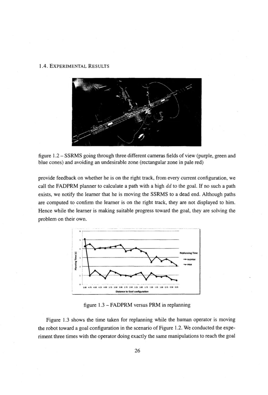
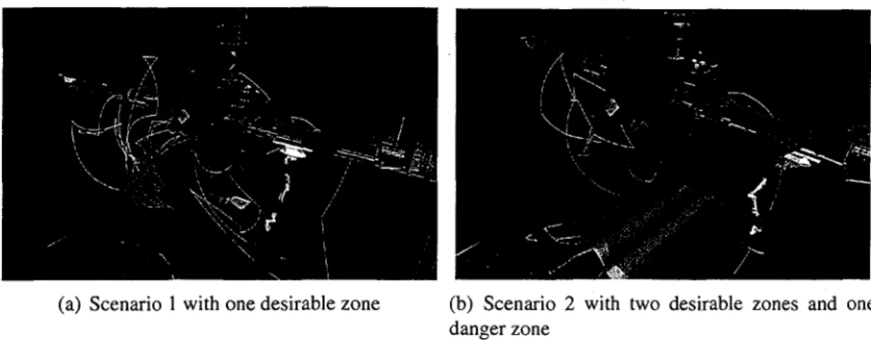
In the SSRMS application, the concept of dangerous and desirable zones is motivated by a real-world application dealing with teaching astronauts to operate the SSRMS in order to move payloads or inspect the ISS using a camera mounted at the end effector. Astronauts have to move the SSRMS remotely, within safe corridors of operations. The definition of a safe corridor is that it must of course avoid obstacles (hard constraints), but also go as much as possible within regions visible through cameras mounted on the ISS exterior (so the astronaut can see the manipulations through a monitor on which the cameras are mapped). Hence, safe corridors depend on view angles and lighting conditions for cameras mounted on the ISS, which change dynamically with the orbit of the ISS by modifying their exposure to direct sunlight. As safe corridors are more complex to illustrate on paper, we just picked conical zones approximating cameras view regions and polygonal zones at arbitrary locations. Figure 1.2 illustrates a trajectory of the SSRMS carrying a load and going through three cameras fields of view (purple, green and blue cones) and avoiding an undesirable zone with very limited lighting conditions (rectangular zone in pale red).
The first experiment illustrates the situation in which a human operator is learning to manipulate the SSRMS from a given start configuration to a given goal configuration. To
1 . 4 . E X P E R I M E N T A L R E S U L T S
figure 1.2 - SSRMS going through three different cameras fields of view (purple, green and blue cones) and avoiding an undesirable zone (rectangular zone in pale red)
provide feedback on whether he is on the right track, from every current configuration, we call the FADPRM planner to calculate a path with a high dd to the goal. If no such a path exists, we notify the learner that he is moving the SSRMS to a dead end. Although paths are computed to confirm the learner is on the right track, they are not displayed to him. Hence while the learner is making suitable progress toward the goal, they are solving the problem on their own.
Figure 1.3 shows the time taken for replanning while the human operator is moving the robot toward a goal configuration in the scenario of Figure 1.2. We conducted the expe-riment three times with the operator doing exactly the same manipulations to reach the goal
5.00 4.7S 4.SO 4.2S 4.00 3.75 3.50 3.00 2.75 2.50 2.2S 2.00 1.75 1 50 1.25 1.00 0.75 0.50 0.25
Oistance to Goal configuration
1 . 4 . E X P E R I M E N T A L RESULTS
from the start configuration and each time using FADPRM (with /3 = 0) and the normal PRM. Except for the first few iterations, FADPRM take less re-planning time than PRM. For FADPRM and in the first few iterations, the overhead incurred by the GAA*-based exploration dominates the planning time. In later iterations, it is outweighed by the savings gained by re-planning from the previous roadmap.
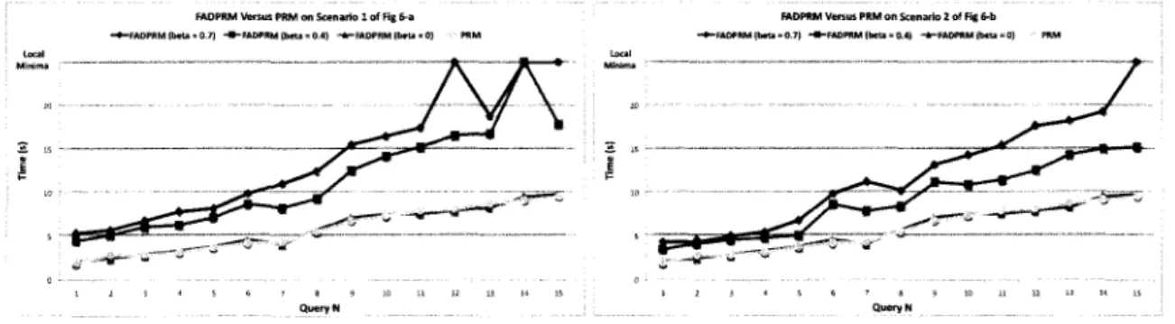
FADPRM Versus P R M - • - F A D P R M (beta = 0.4) • • • F A D P R M (beta=0) PRM 0 • •• -1 2 3 4 5 6 7 8 9 -10 -1-1 -12 -13 -14 -15 Q u e r y N
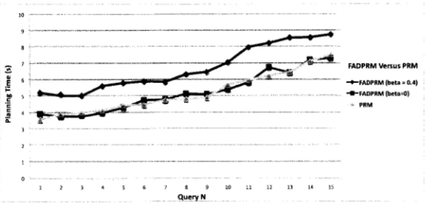
figure 1.4 - FADPRM versus PRM in planning time
In Figure 1.4, we compare the time needed for FADPRM and PRM to find a solution for 15 arbitrary queries in the ISS environment. Since the time (and path quality) for finding path is a random variable given the random sampling of the free workspace, for each query we ran each of the planners ten times and reported the average planning time. In this case, FADPRM is used in a mode that does not store the roadmap between successive runs. Before displaying the results, we sorted the PRM setting in increasing order of complexity, starting with queries taking less time to solve.
For FADPRM, we show results with (3 = 0 and /3 = 0,4. With (3 = 0, FADPRM behaves exactly like the normal PRM. With f3 = 0,4, planning takes more time for both planners. This validates our previous analysis about FADPRM : with (3 = 0, an FADPRM planner behaves in way very similar to a normal PRM, but as soon as we start seeking optimality (in our case with f3 = 0,4), the time for planning will increase proportionally.
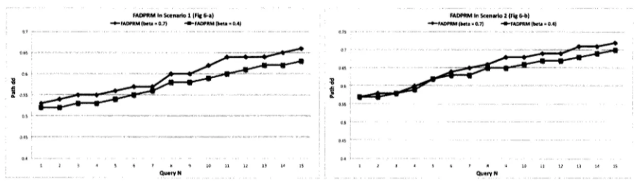
On an other hand, Figure 1.5 shows that (3 = 0,4 yields higher quality paths than (3 = 0. This validates another previous analysis : higher (3 values yield better paths, but take more time to compute.