Record Number: 16030
Author, Monographic: Cluis, D.//Laberge, C. Author Role:
Title, Monographic: Rationalisation for regional trend detection of the CWS/LRTAP monitoring network at Algoma, Muskoka and Sudbury sites
Translated Title: Reprint Status: Edition:
Author, Subsidiary: Author Role:
Place of Publication: Québec
Publisher Name: INRS-Eau
Date of Publication: 1997
Original Publication Date: Avril 1997
Volume Identification: Extent of Work: ii, 104
Packaging Method: pages incluant 4 annexes
Series Editor: Series Editor Role:
Series Title: INRS-Eau, rapport de recherche
Series Volume ID: 493
Location/URL:
ISBN: 2-89146-468-0
Notes: Rapport annuel 1997-1998
Abstract: Rappport rédigé pour Environnement Canada, région de l'Ontario
Call Number: R000493
RATIONALIZATION
FOR REGIONAL TREND DETECTION
OF THE CWSILRTAP MONITORING NETWORK AT ALGOMA, MUSKOKA AND SUDBURY SITES.
RATIONALIZATION FOR REGIONAL TREND DETECTION OF THE CWSILRTAP MONITORING NETWORK AT ALGOMA, MUSKOKA AND SUDBURY SITES.
Contract # KR405-6-0162
Environment Canada CWS ,Ontario Region
LRTAP Program
by
Daniel Cluis and Claude Laberge
INRS-EAU
Report # 493 April 1997
ABSTRACT
This report presents the results of a rationalisation of the CWS/LRT AP network of lakes of the Muskoka, Algoma and Sudbury regions, monitored since 1988 to assess the recovery from acidic precipitations on a regional basis. The purpose of the study is to propose efficient strategies for the reduction of the sampling effort minimizing the loss in power of the network, to be reduced as a consequence of financial cutbacks.
Starting with the 1988-1995 database, the historical spatio-temporal persistence, known to reduce the information content of the individual measurements and the power of trend detection techniques are first evaluated for the six most important parameters of the database: pH, Alkalinity, Base cations, Sulfates, Dissolved Organic Carbon and Nitrites-Nitrates.
The virtues of competing logistic strategies for the considered sampling effort reduction are discussed and compared. Then the choice of a sampling strategy is made, taking into account the inter-lake variabilities as demonstrated by the historical measurements and the resulting power of the reduced networks is evaluated for different sampling efforts.
Finally, a procedure is described, leading to the actual selection oflakes to be sampled on recurring cycles, according to their relative distances and to the external classification to which they belong.
TABLE OF CONTENT
INTRODUCTION 1
CHAPTER 1: Spatio-temporal variability of historical data 3
1.1 Localisation of the sampling stations. 3
1.2 Assessment of spatial and temporal persistence. 5
1.2.1 Spatial persistence. 6
1.2.2 Temporal persistence. Il
1.3 Conclusions. 14
CHAPTER 2: Sampling strategies 16
2.1 Statistical considerations about the CWS/LRT AP network. 16
2.2 Historical sampling. 17
2.3 Strategies. 18
CHAPTER 3: Power analysis of sampling strategies 19
3.1 The independent case. 19
3.2 Choice of an "optimal strategy" 22
3 .2.1 Muskoka site. 23
3.2.2 Algoma site. 23
3.2.3 Sudbury site. 24
3.3 Selected sampling strategy. 25
3.4 Further development for the selected sampling strategy. 25
3.4.1 Discussion on spatial correlation. 25
CHAPTER 4: Rationalization 29
4.1 Selected sampling effort. 29
4.2 Effect of the spatial correlation on the power for the chosen sampling strategy. 34
4.3 Procedure for the choice of stations for future monitoring. 34
4.4 Actual selection oflakes. 34
Appendix A-l: Interlake distances.
Appendix A-2: Proximity counts, geophysical classification and historical sampling of lakes (by cluster or region).
Appendix A-3: Detection power of the historical network for different future sampling efforts at the 3 sites.
Appendix A-4: Selection oflakes and groupings.
INTRODUCTION
SCOPE OF THE PRESENT CONTRACT
The purpose ofthis contract is to help redesign the CWS/LRTAP biomonitoring network ofwater quality from lakes located in 3 sites (Sudbury, Muskoka and Algoma).
The network, sampled once a year in the fall, was established in 1983 to monitor the eventual recovery with time of lakes vulnerable to acidity, following the reduction of atmospheric acidic compounds. In previous studies, we have assessed the power of the network to detect trends on a regional basis; we have also performed sorne multivariate analyses to regroup lakes and parameters ofsimilarbehaviours. One of the key points of the statistical analyses was the estimation ofboth the temporal and spatial persistence of the data, which controls the power to detect changes and thus validates the use of various parametric or nonparametric techniques according to their pertinent underlying assumptions.
This contract was triggered by the necessity, resulting from imposed financial cutbacks, to reduce the number oflakes to be sampled each year; during the period 1990-1994, the average sampling effort was of 331 lakes a year; for the period 1990-1995, it was of 388 lakes. The goal for the future sampling effort was to reduce it to an order of magnitude of200, while minimizing unavoidable los ses in the trend detection power of the network. In the past, 260, 253 and 161 lakes were sampled respectively in the Muskoka, Algoma and Sudbury regions, but Dot on a yearly basis.
Two main questions will be addressed: -Which sampling strategy should be chosen:
.Round robbin: all sampling efforts in one region each year, with rotating region with the years . . Split sampling: 1/3, 1/3, 1/3 oflakes of each region sampled each year, with a rotation with the years .
. Sorne combination ofboth.
-Which lakes should be kept in the network in view of their representativity and of their belonging to sorne extemal classification modalities, while giving an overweight to small, quick reacting lakes, the main object of the monitoring. The objective here is to retain about 80% of lakes smaller than 10 ha. Lakes to be reduced in number should preferably belong to:
CLASSMA: class 1, value >4 CLASSUD: class 4, value = 4 CLASSUD: class 4, value = 0
As a consequence, what is the loss in trend detection power, i.e. in the ability to detect trend expressed as a fraction of the intrinsic variability, let say 0.5
a ,
with a given power, nine times out often, for the network redeveloped with 3 cutback hypotheses, i.e. approximately 180, 195 and 210 retained lakes, to be sampled each year ?In the following report, we will refer to results obtained previously on the same database by our previous studies, shortly as:
RI: Linear trend detection and statistical power analysis. Lakes from the Sudbury area (1983-1994) .. Contract # KR405-4-0276, March 1995.
R2: Comparisons of lake medians and lake trend slopes in the Muskoka, Algoma and Sudbury regions. Contract # KR405-5-0159, March 1996.
R3: Regional trend detection and power analyses for chemical parameters monitored at the CWS LRTAP biomonitoring sites in Algoma, Muskoka and Sudbury (1988-1995), Contract #KR405-5-0179, May 1996.
STRUCTURE OF THE REPORT
The present report will first locate the sampled lakes at the 3 sites: Muskoka (1); Algoma (12) and Sudbury (37) and determine their relative distances using UTM coordinates. 6 quality parameters are used for this rationalisation study: pH, Alkalinity, Basecations, S04, DOC and N02-3. Three sets of data will be used for the analyses: Two concerning the levels of the parameters recorded at the start of the pro gram ( years 93, 88 and 91 respectively) and the last available year ( 95). One related to the evolution of the measurements as defined by the average yearly trend slopes.
Chapter 1 studies the persistence of the historical data set. It is well recognized that both spatial and temporal persistences reduce the regional power of a trend monitoring network as the Information Content of each data is reduced by redundancy: Part of the new information is already contained
in past information at the sampled station, and also in information gathered at nearby stations. In this chapter, the study of historical data set will allow to draw conclusions that will be applied to the rationalisation process.
Chapter 2 evaluates the possible sampling strategies and Chapter 3 quantifies their associated detection power. Finally, Chapter 4 proceeds with the rationalization proper, i.e. the evaluation of the future sampling effort compared with the historical one, the choice of the lakes to be monitored and the definition of their sampling cycles.
CHAPTERI
Spatio-temporal variability of historical data.
1.1 Localisation of the sampled stations.
The sampled stations are located within 3 regions (1=Muskoka; 12=Algoma and 37=Sudbury). Given the UTM coordinates of the stations, it is possible to draw a global map of the location of the stations. Even if the maps are not very clear, due to the high number of lakes and their proximity, these map give a good pattern of their dispersion. In the following figures, the coordinates are expressed as km (UTM). The Muskoka and Algoma regions (260 and 2531akes, respectively) exhibit selected c1usters ( called "plots")oflakes located within 5 x 5 km squares and the Sudbury region (161 lakes) shows a good spreading oflakes within the territory.
Figure 1-1 Location of the sam pied lakes in the Muskoka region .
....
5051f -" .. ,
... I.I"'!
... '1'1...
5045eJt.iJ
5039~
5033 0 ) .~ 5027 .s:-
.... oz
5021 5015 5009 , ,~ 5003\1
..
~
...;
~..
4997'-'I:<...I---+-~---'----I-'--+--~--'-'
657 661 665 669673 677 681 685 689 693 EastingFigure 1-2 Location of the sampled lakes in the Algoma region.
5234
5227
5220
•
:m
5213
c-•
.c
5206
-
...
0Z
5199
•
5192
Si
5185
5178
5171
670 679 688 697 706 715 724 733 742 751
Easting
Figure 1-3 Location of the sam pied lakes in the Sudbury region .
•
5209
t
-1
•
52054~,
,,"
•
•
•
••••••
....
5201
t-.-
-
...
•
•
•
•
••
.-,
If.
•
•
•
5197
r-i
tC ••
•
•
•
••
4 (J)••
L:t.
•
•
•
--•
•
•
.,
L: fi' -1-1•
•
L.5193
r-):
•
0-
•
-
•
•
Z••
••
•
•
•
5189
t-••
,.
•
~
-.\'.p
•
5185
t-••
-5181
r-I
5177
:~
1 1 1 1 1 1 i502 506 510 514 518 522 526 530 534 538 542
Easling
As we will be interested by lakes influenced by each others, the tables A-l, (given in Appendix A and regrouped in clusters for the Muskoka and Algoma regions and in East-West strips in the Sudbury region) provide the distances between lakes within each cluster; In these tables, interlake distances lower than 4, 3 and 2 km (see la ter in this chapter for justification), respectively for the Muskoka, Aigoma and Sudbury regions have been shaded as the se criteria will be used later as a factor to eliminate sorne of the lakes due to spatial persistence_
1.2 Assessment of spatial and temporal persistence.
In a network devoted to detect trend regionally, the information contained in a sample is not completely new, as part ofthis information is also contained in synchroneous data gathered at other nearby stations (spatial correlation) , and spills over to the previous and next samples gathered at the same station (temporal correlation). Thus, a new sample may contain redundant information. Knowledge of both structures is essential for the estimation of the power of the trend detection network. As mentioned by Loftis et al. ( Loftis, lc., G.B.McBride and lC.Ellis, 1991, "Considerations on the scale in water quality monitoring and data analysis". Water resources bulletin, 27-2:p.255-264):
... "The question of wh ether a given series of equally spaced observations are independent or serially correlated is scale dependent in many situations" ... This statement applies both to temporal and to spatial dependence. In the present report, scale plays an important role in determining the dependence of sampled observations. In the case of temporal dependence, it seems logical to accept that observations taken from the same lake of high flushing rate are independent when at least a full year separates them. It would be more hazardous to suppose that weekly observations are independent. In the case ot spatial dependence, the scale effect should also be taken into account to make sure that the conclusions drawn are pertinent. Regional trend detection implies working within a region where lakes might be spatially correlated. A spatial correlation between two lakes within the Sudbury region could be considered as important for a trend detection study at the scale of the whole Ontario Province, even more at the scale of the country ( Canada), but it should be seen as only a normal intrinsic occurrence for the Sudbury region.
It is then quite normal that closeby lakes appear correlated within the same region, and it seems logical that this intrisic correlation would not affect the trend detection tests associated with this region. But in the case of the Muskoka and of the Algoma regions, the spatial correlation problem is looked at another scale. In these regions, sampled lakes were chosen within 10 km x 10 km c1usters ( called "plots"). The selection oflakes this close from each others brings inevitably higher correlations as the intrinsic regional correlations of the whole entitie. This "overweight"correlation between nearby lakes constitutes what will be called in this text "spatial correlation"in so far as it is closely distance-related.
1.2.1 Spatial persistence
The analysis of spatial data constitutes a branch of the statistics called geostatistics. One classical problem, called Kriging or optimal interpolation, deals with the evaluation of probable values at sorne place (with confidence levels) in a field, given only a few sampled points. The spatial persistence structure is studied using as tool the variogram, a graph very similar to the autocorrelogram in the temporal domain, where aH pairs of sampled points are combined in lagged classes, according to their spatial distances (spatiallag). In the Kriging, the shape ofthis variogram is compared with shapes associated with theoretical models of decaying apatial memory (spherical, exponential, linear or random structures) and the recognized experimental structure is then used to evaluate values at unsampled points. In this application, we will only use this mathematical tool to assess the extend of spatial dependency.
The variogram is characterized by 3 values: the nugget corresponding to the intercept (the extension) of the variogram shape at lag 0 on the variance axis, i.e. the intrinsic variability related to very close measurements, the sill corresponding to the asymptotic level of the global variance of unrelated, far apart, points and the range which is the spatiallag where the variogram reaches this plateau of spatial independency. The difference level between the sill (standardized to 1 in the following example and in the table ofresults) and the nugget represents the part of the variability affected by spatial persistence. In our case, we will interpret the range as the distance within which samples contain sorne distance dependent common information.
Figure 4 presents a typical experimental standardized variogram (pH omnidirectional , Sudbury region, 1995) and the information it contains: the range is of about 6 km, the nugget is of 0.35 and the spatial correlation coefficient r, obtained for h=range/3 (here h=2km) is about 0.6.
Figure 1-4 Typical standardized variogram (pH, Sudbury region, 1995)
')S
(lhl)
1.2
1
0.8
0.6
0.4
0.2
0
0
4
8
12
16
20
24
28
Ihl
When used for Kriging, the experimental variograms have to be identified with the shape of sorne theoretical models (spherical, exponential, Gaussian or Power, with or without nugget effects). This is not our purpose with this project as we are only looking for the extend and magnitude of possible spatial redundancy. In addition, we have also investigated the strength and extend of possible spatial cross-correlation between parameters within regions.
Tools used
To perform the variogram analyses, we have used Variowin 2.2 (Pannatier, 1996), a very new Windows version of the classical EPA geostatistical software GEOEAS (Englund and Sparks, 1981), which was working under the DOS operating system.
Spatial variability (for each parameter)
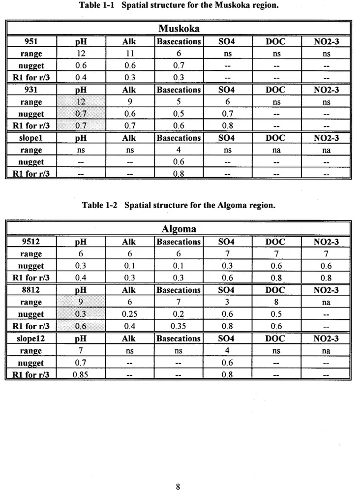
The following tables present the results gathered by region; ns means no spatial structure and na means that data were not available.
9512 range nugget RI for r/3 8812 range RI for r/3 slooe12 range nugget RI for r/3
Table 1-1 Spatial structure for the Muskoka region.
Muskoka
N02-3
ns
Table 1-2 Spatial structure for the Algoma region.
Aigoma
pH Alk n. tlium S04 DOC N02-3
6 6 6 7 7 7
0.3 0.1 0.1 0.3 0.6 0.6
0.4 0.3 0.3 0.6 0.8 0.8
pH Alk"" tliOIl~ S04 DOC N02-3
na .J~ 0.4 0.35 0.8 0.6 pH
~==A=I=k==~B=a=se=c=at=io=n=s*=~SO~4==9==~DO==C==~==NO==2-3==91
7
m
m
4
ns
na 0.7 -- -- 0.6 0.85 -- -- 0.8--
--Table 1-3 Spatial structure for the Sudbury region.
0.35 0.6
RI for r/3 0.7 0.85
3 3 ns ns
0.65 0.8
In the Muskoka region, the range is large (up to 12 km) for sorne parameters; in the Algoma region, the maximum range is reduced to 9 km and in the Sudbury region, it is even smaller (6 km). In the 3 regions, the slopes present very little spatial structure and the levels of the nugget is high as
% of the total variance. Thus, this indirect secondary variate can be considered as completely spatially uncorrelated.
Taking the worse case situation of all parameters, years and variates, one can conservatively assess the spatial radius of influence to one third of the maximum range for the region and for the whole set of parameters:
In the Muskoka region, 4 km with a spatial correlation coefficient ofr1=O.7
In the Algoma region, 3 km with a spatial correlation coefficient ofr1=O.6 In the Sudbury region, 2 km with a spatial correlation coefficient ofr1=O.8
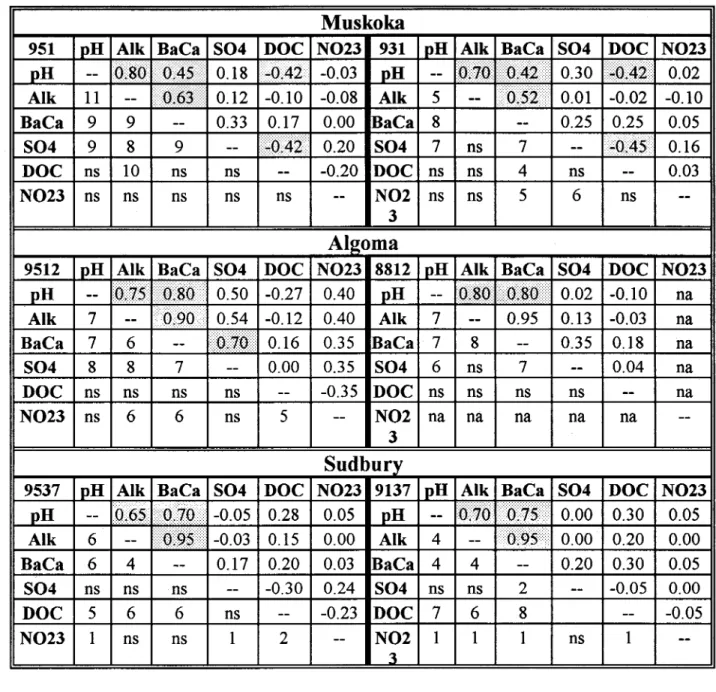
Spatial covariability between parameters
In order to assess the spatial covariability of the six selected parameters, we also used Variowin 2.2 the cross variograms and the lagged cross-correlations between parameters.
Table 1-4 Spatial covariability between partameters.
Muskoka
951 pHA1k
1
B.C.1
S04 DOCN!m
931 pH Alk BaCa S04 DOC N()23 pHQ(SQ
0.181-()42 •• ·•
-0.03 pH--
Q.îQ
••••••• Ô.4.î ••
0.30 1 ...••••••••••• 0.02 Alk 11 -- 0.12 -0.10 -0.08 Alk 5--
Q.{jg;
0.01 -0.02 -0.10 BaCa 9 9--
0.33 0.17 0.00 R".C'". 8--
0.25 0.25 0.05 ... S04 9 8 9--
IŒp,4-~ 0.20 S04 7 ns 7--
1+1),.4' 0.16 DOC ns 10 ns ns--
-0.20 DOC ns ns 4 ns--
0.03 N023 ns ns ns ns ns--
N02 ns ns 5 6 ns --3Aigoma
9512 pH Alk BaCa S04 DOC N023 8812 pH Alk BaCa S04 DOC N023 pH
--
Ih;;;':;';'
.1 .... .. · ... IIRÛ.· 0.50 -0.27 0.40 pH--
ViP\! .. ViP!:} 0.02 -0.10 naAlk 7
--
1 ŒYU./ 0.54 -0.12 0.40 Alk 7--
0.95 0.13 -0.03 naBaCa 7 6
--
iQ.jQ 0.16 0.35 BaCa 7 8--
0.35 0.18 naS04 8 8 7
--
0.00 0.35 S04 6 ns 7--
0.04 naDOC ns ns ns ns
--
-0.35 DOC ns ns ns ns--
naN023 ns 6 6 ns 5
--
N02 na na na na na--3
Sudbury
9537 pH Alk BaCa S04 DOC N023 9137 pH Alk BaCa S04 DOC N023 pH
--
IQ,6~ 1· ••• ··O.jQ) -0.05 0.28 .. 0.05 pH--
IÔl'7Q
IÔ.7S •••••• •
0.00 0.30 0.05Alk 6
--
1 •••••• 0)95 •• • ••••• -0.03 0.15 0.00 Alk 4--
i>0.95· •• •
•••
0.00 0.20 0.00BaCa 6 4
--
0.17 0.20 0.03 BaCa 4 4--
0.20 0.30 0.05S04 ns ns ns
--
-0.30 0.24 S04 ns ns 2--
-0.05 0.00DOC 5 6 6 ns
--
-0.23 DOC 7 6 8--
-0.05N023 1 ns ns 1 2
--
N02 1 1 1 ns 1--3
On these tables, the upper right triangles presents the global levelof correlation between the parameters, and the lower left triangles present the radius of influence (in km) of the more intimate relationships. The cells of the higher values are shaded and consistently demonstrate a close relationship between pH and Alk, pH and BaCa, BaCa and Alk. The range of influence, shown in the lower triangles are of the same order of magnitude as the ranges established in the previous section. The results for the slopes are more erratic, but nevertheless exhibit high values for the same combinations of parameters:
Muskoka Algoma Sudbury pH - Alk 0.45 0.52 0.27 pH -BaCa 0.50 0.22 Alk - BaCa 0.35 0.55 0.7 Alk - S04 -0.40 -0.24 pH - S04 -0.60 -0.45 -0.20 BaCa - S04 0.50
Closing this section, one could add that, for more in-depth purposes, the spatial tools used here could certainly be re-used with success in analysing the spatial behaviour, when applied not on the totality of the lakes of each region as was done here, but_on members of the different classifications of lakes related to their geology, volumes and other geophysical attribut es and as such, add to the interpretation of the recovery of the lakes of the region ...
1.2.2 Temporal persistence.
Even if the presence of temporal persistence seems unlikely in our case of samples taken once a year or once every two years on lakes with yearly turnover, statistical analyses were performed to ensure that this possible dependance has no significant effect on trend detection results.
A first analysis was performed in our R3 report to determine the possible presence of temporal autocorrelation in the data obtained trom the 3 regions. In this first analysis (R3, table 86, page 37) the correlation between pairs of years has been studied for the lakes of the Muskoka region. This analysis allows only to determine the maximum level of autocorrelation, because, as discussed in R3 report, " ... , this correlation contains a part related to the levels of the parameters of the lakes. A lake presenting, for a parameter such as pH, a level higher in 1990 than the bulk of the other lakes will probably have also higher values for the other years"
Thus the occurrence ofvery close values for two consecutive years seems more related to their origin from the same lake than to possible temporal persistence.
A second analysis performed for the Muskoka region, in the same report (R3, table 87, page 38) shows that the random sampling of a single value per lake (eliminating the possibility of temporal persistence) yields very similar results as the ones obtained by the use of all the data available for each lake.
Table 1-5 Trend detection using regressions using one observation per lake vs using ail observations for alilakes (Muskoka region).
1 observation per lake Ali observations for each
lake
Parameter n RMSE Siope Estim. Estim. n RMSE Siope Estim.
1990 1995 1990 5.57 27.08 Estim. 1995 6.02 20. 74 Alkalinitv 228 26.97 1.2100 16.93 23.00 772 29.00 0.900 19.96 24.46 Calcium 235
0.65:-(),llQQ
2.19 1.64 790 0.551"1"lh8 2.22 1.6CIMapnp~illm 235 0.20ISQ.()2QO 0.63 0.48 790 0.181+ŒIJ]:$ 0.67 0.51
Potassium 235 0.12 0.0000 0.33 0.33 790 0.13 -0.002 0.34 0.33
Sodium 235 0.94 -0.0150 0.76 0.68 790 0.92 -0.032 0.81 0.65
Sulfate 235 2.01 iJ
b.53Qg
7.04 4.37 7901.73IJà~--6.-93-t--4-.3-S"
Silicate 235 1.23 Il 1 I!Jt 1.20 1.74 790 1.221ULpmm 1.25 1.66Chloride 235 1.62 -0.0010 0.46 0.46 790 1.54 -0.028 0.52 0.38
TIC 135 0.34~Q 0.83 0.54 464 0.36 -0.015 0.65 0.58 DOC 204 3.13 0.0370 6.00 6.19 693 2.96 0.010 5.97 6.03
It--N_~_~_N_O_3--;-~_~_:i-_~_:_~~-tI_±_oÔ_·.O()_03_·.t·~-t4Qr--_~_:~-~i--~_:~-~+-:_:~-+--~-:~-~r= -1t---~-:~-~;---~-:~--i~1
TN
69 0.12 n.a. 0.38 0.38 231 0.16 n.a. 0.40 O.4CNH3
135 37.71 -0.2400 31.83 30.64 464 36.55 -0.690 37.06 33.62 TP 204 9.14 ..1.ô(iôÔ
13.12 7.82 690 11.48 (HE170 13.51 7.66 Shaded areas are ass('~iateè to siQnificant slooes at the 5% s\Qnificant levelOne can note that:
al The results related to trend significance are similar except for TIC and N02N03.
bl The RMSE and location parameters (ordinate at the origin, slope, estimated values for 1990 and
1995) are consistent from one analysis to the other.
The similarities in results of the se analyses allows the following important conclusions:
al The possible autocorrelation has a negligible effect on trend detection conclusions iflakes of the Muskoka region are sampled annually, bi-annually or tri-anually. As a consequence it is proper to use all the available years for regional trend detection.
bl In a network rationalisation scheme, the similarity in results suggests that the number of lakes sam pied each year can be reduced and that a sufficient temporal trend detection power would be retained.
Even though the analyses performed in previous reports tend to conclude to the absence of an auto correlation effect on the conclusions of the trend detection analyses, no attempt has been performed to evaluate the significance of the first order autocorrelation coefficient in studied regions. The main reason for not estimating the first order autocorrelation coefficients was the short lengths of the series and the non-equidistance of the observations for the Muskoka and Algoma regions. However, an attempt is now performed with the data of the Sudbury region where equidistant observations are available during 6 consecutive years (1990-1995) for a group of 49lakes. Three parameters are studied: pH, sulfates and alkalinity. Given the fact that trends affect the autocorrelation coefficient, the estimation of this parameter has been performed on detrended data. Table 1-6 presents the Durbin-Watson (DW) statistics used to test the presence ofa positive first order autocorrelation coefficient. Regretfully, this test is not recommended for short series and critical values are only tabulated for series larger than 14. Durbin-Watson statistics should only be regarded as indicators of the possible presence of autocorrelation. Given the small size of the series treated here (n=6), a significant autocorrelation can be suspected for Durbin-Watson statistics smaller than 1.0.
Table 1-6 Durbin-Watson statistics and estimated first order autocorrelation coefficient of simple Iinear for trend detection in the Sudbury re~lOn.
pH pH Alkalinity Alkalinity 804 804
Lac Number DW 8tatistic ri DW 8tatistic rI DW 8tatistic ri
2 l.99 -0.10 l.64 -0.12 l.80 -0.14 3 l.87 -0.05 2.24 -0.19 2.11 -0.24 5 l.56 -0.06 2.38 -0.32 2.15 -0.14 13 l.13 0.15 l.57 0.09 2.32 -0.20 16 l.98 -0.16 2.34 -0.32 l.46 0.09 17 l.02 0.22 1.41 0.19 2.32 -0.30 22 2.38 -0.28 2.45 -0.34 2.55 -0.40 197 3.10 -0.62 3.25 -0.66 l.44 0.04 199 2.66 -0.46 2.04 -0.21 2.48 -0.46 219 3.41 -0.73 3.27 -0.70 2.12 -0.15 225 l.52 -0.04 1.27 0.11 2.70 -0.50 240 l.52 -0.03 1.63 0.00 2.00 -0.16 247 2.11 -0.31 2.37 -0.39 3.15 -0.61 248 l.61 -0.05 2.08 -0.14 1.35 0.20 250 1.57 0.11 1.45 0.18 2.57 -0.47 251 2.70 -0.55 3.38 -0.75 1.39 0.13 254 2.73 -0.54 3.05 -0.58 3.19 -0.65 257 l.89 -0.23 1.86 -0.17 2.70 -0.50 258 1.31 0.12 l.26 0.17 l.44 0.09 259 1.30 0.05 l.27 0.05 2.23 -0.40 266 2.79 -0.49 3.20 -0.60 2.07 -0.22 268 2.24 -0.27 2.91 -0.49 3.47 -0.74 299 1.61 0.02 1.75 -0.05 l.l5 0.26 316 1.36 0.13 2.23 -0.21 3.55 -0.81 333 2.56 -0.50 2.29 -0.30 l.90 -0.12
pH pH Alkalinity Alkalinity S04 S04
Lac Nurnber DW Statistic ri DW Statistic ri DW Statistic ri
338 2.14 -0.27 1.85 -0.07 2.67 -0.47 401 2.30 -0.34 2.92 -0.48 1.86 -0.11 402 1.93 -0.21 1.68 0.10 2.48 -0.33 403 1.52 -0.08 1.06 0.21 2.07 -0.15 404 2.11 -0.13 2.20 -0.13 3.07 -0.55 407 1.57 -0.11 1.50 0.14 2.91 -0.51 408 1.88 -0.20 1.38 0.15 3.21 -0.66 409 3.11 -0.65 2.85 -0.54 1.82 -0.09 410 3.10 -0.68 2.75 -0.50 2.57 -0.50 524 2.91 -0.47 2.99 -0.57 1.98 -0.24 527 2.17 -0.22 2.56 -0.32 2.57 -0.30 530 2.40 -0.24 2.52 -0.28 2.19 -0.11 583 1.28 0.11 1.64 0.06 2.90 -0.60 589 1.67 -0.10 2.19 -0.14 1.76 0.00 590 1.56 0.02 1.72 0.04 1.14 0.20 593 2.25 -0.36 2.03 -0.13 2.07 -0.21 856 2.95 -0.63 3.19 -0.67 2.33 -0.28 900 1.13 0.13 1.24 0.16 2.73 -0.37 902 2.47 -0.30 3.02 -0.56 2.39 -0.29 905 2.22 -0.38 2.05 -0.13 1.31 0.20 909 1.94 -0.24 2.19 -0.20 1.54 -0.01 920 1.07 0.18 1.45 0.11 1.78 -0.03 922 2.61 -0.50 2.32 -0.40 2.06 -0.16 932 1.33 0.08 2.68 -0.34 1.82 -0.02
Table 1-6 shows that no lake, for any parameter, exhibits a DW statistics lower than 1.0. Furthermore the estimators for the order-l autocorrelation coefficients are quite often negative (76%, 69% and 82% of aIl cases for pH, alkalinity and sulfates respectively) and never larger than 0.26. Even if the previous results have been obtained in the context of very short samples, they nevertheless enforce the validity of the hypothesis ofno temporal persistence, for yearly or bi-yearly samplings. In face of these results and the actual unavailability of larger samples, we will in the following parts accept the hypothesis that temporal persistence has a negligible effect on the detection of trends, thus on the rationalisation of the network of lakes, and this, by extension, in the 3 regions.
1.3 Conclusions
In this chapter dealing with the spatio-temporal persitence ofhistorical data, we have established or infered by induction:
Secondly, that spatial existence was present, but that the radius of influence where spatial persistence contains significant redundancy in information is limited to 4, 3 and 2 km for the Muskoka, Algorna and Sudbury regions. As a consequence, we have classified in descending order the lakes, in each cluster, for the Muskoka and Algorna regions and for the whole Sudbury region, according to the nurnber of other lakes present in their radius of cornrnon information. It has been verified that this order was almost the sarne as if the worse lake was first identified, eliminated, and then the distances of the rernaining lakes recounted to identifY the second worse, an so on. This caveat, because it was at first believed that, given the fact that one distance affects 2 lakes counts, elirninating the first rnost close lakes, other nearby lakes could possibly have biased counts of proxirnity, which was not the case.
A synthesis of the result is given at in the Appendix A-2 as Tables M-22/25, A-23/27 and S-24 , for the Muskoka and Algorna clusters and for the whole Sudbury region. The tables contain the narne of the lake, the nurnber of other lakes within their radius of influence, the classification criteria and the nurnber of years the lake was sarnpled for further use.
CHAPTER2 Sampling strategies 2.1 Statistical consideration about the CWS/LRTAP network.
The databank provided by the CWS presents several characteristics that must be taken into account in the rationalization process. First, and this is particularly true for the Algoma and Muskoka regions, lake selection wasn't done with a completely random sampling. As we see it, lake selection in the Algoma and Muskoka regions was conducted according to a simple c1uster sampling: Random choice of 7 clusters (plots 5km x 5 km) in the Muskoka region and of 9 clusters in the Algoma region, followed by the selection of alliakes located in each of the clusters. This sampling method needs special variance estimators since the use of several units (lakes) spatially near from each others will usually underestimate the target population variance.
To better understand the consequences of such an historical sampling scheme, a short discussion on the target populations and on the sampled lakes will be presented:
In the present report, three regions are studied. These regions are aIllocated in (or in the vicinity) of what is called Northern Ontario. Collectively, they could be used to assess the detection of regional trend for Northern Ontario, giobally speaking. The target population could then be: ail smalliakes in Northern Ontario, but the selection oflakes at three sites located near Sault Ste. Marie, Sudbury and Hunstville would surely underestimate the target population variance and probably be biased for level parameters (means and trend slopes) since no lake would be sampled between Sault Ste. Marie, Manitoba and the north of Thunder Bay ..
If the three studied sites are to be used giobally to produce a regional trend detection, the target population should be: ail sm ail lakes located in Ontario between Sault Ste. Marie and the Algonquin Provincial Park. The three sites cover a good part of the region defined above and should give unbiased estimates for level parameters (means and trend slopes). However, special care must be taken to the variance estimates since lakes are grouped at only three sites, with probably less variability than in the target population. In addition, in two of these three sites, the lakes are grouped within plots, with probably less variability than in their complete respective regions. The three sites could also be studied separately :
1/ Given the presence oflakes weIl scattered in the Wanapitei study area (50 km North of Sudbury), the target population can then be defined as: ail small (to be quantified .. ) lakes located in an area of approximately 30km by 30 km: 900 km2. The goal of a regional trend detection would then
be to evaluate the statistical significance of changes in this area for different chemical parameters. Although the conclusion of a regional trend detection analysis does not allow to draw conclusions for individuallakes, regional trend detection can be quite useful when long enough time series are not available for individuallakes. The use of severallakes regionally compensates, in part, for the shortness of temporal series: one is trading the lack of one long time series at an individual site which could give significant trend detection results, for shorter multiple regional stations. As the selected lakes cover the complete region, their mean values and variances should be unbiased estimators of the target population mean and variance.
2/ The 7 plots of the Muskoka region are located in an area of approximately 3000 km2
. The target
population is then defined as: ail smalllakes (to be quantified .. ) in that area. Inside the region, lakes are selected according to a simple cluster sampling. Spatial correlation analysis shows that lakes spatially close tend to be more correlated than lakes far apart. Thus, the original sampling plan tend to underestimate the target population variance and let trend detection tests conclu de too often that a (significant) trend exists for the target population. This should be taken into account in regional trend detection at this site.
3/ The 9 plots of the Muskoka region are located in an area of approximately 2000 km2
. The target
population is then defined as: ail smalllakes ( to be quantified .. ) in that area. Inside the region, lakes are selected according to a simple cluster sampling. Spatial correlation analysis shows that lakes spatially close tend to be more correlated than lakes far apart. Thus the original sampling plan tend to underestimate the target population variance and let trend detection tests conclude too often that a (significant) trend exists for the target population. This should be taken into account in regional trend detection at this site.
The rationalization strategies and optimization will be done according to site characteristics and the following working hypotheses.
1/ No temporal autocorrelation on a yearly basis sampling
2/ Spatial correlation is present and its effect should be considered in order to evaluate the possible effect of selecting severallakes too close together.
3/ Variance stationarity in time (years added would not increase or decrease the variance around the trend slope : RMSE).
4/ Eventual trends are monotonic.
5/ Lakes sampled must be chosen from the already sampled lakes. No new lakes can be added.
2.2 Historical sampling
In the past, 260, 253 and 161 lakes have been sampled in the Muskoka, Algoma and Sudbury regions, for a total of 674 lakes, but not on a yearly basis. The sampling effort was averaging 331 lakes a year between 1990 and 1994, and 646 lakes a year in 1995-96. The purpose of the rationalisation is to reduce this number to the order of magnitude of 200, while minimizing the loss in trend power detection, taking into consideration the information contained in the already acquired data. From the previous chapter and our
ru
report ( Tables 91, 92 and 93, pages 44 and 45), it was found that the lakes of the Sudbury region exhibited the large st spatial variability ( see MS lake vs MS year, in the tables), the lowest radius of influence, and in addition, the longest sampled series. At the opposite, the Muskoka and Algoma regions are showing the largest redundancy in information related in part to the historical choice to sample lakes within 5 km c1usters ( so called "plots"). Forthis reason these two regions are the more likely candidates for lake number reduction without losing much information.
2.3 Strategies
Regional sampling provides different types of information:
- Synchroneous measurements provide a spatial picture of the region.
- Successive measurements of the same lakes of a region allow to determine the hydro-meteorological characteristics with time. We will calI this information the "year"effect.
- Long term trend and its associated detection power is related to the length of the sampled series and to the information content of the data.
In this situation, 2 broad classes of strategies can be considered: • The sampling of one region each year, with a return after 3 years.
This strategy gives a detailed spatial picture of the region every 3 years, with lots of spatial redundancy, especially in the Muskoka and Algoma regions, misses the "year"effects for the non-sampled, intermediary years. As a consequence, a regional diagnostic regarding the recovery can only be performed every 3 years for a particular region .
• The sampling of every region each year, but only with a limited number of lakes; different lakes being sampled each year on a regularly rotating basis. In this scheme, the lakes sampled in a region for a particular year should be chosen to be as independent ( far apart) from each other as possible: For the same region, the lakes chosen for the next year will be different from the first set and also chosen to be as dispersed as possible and so on until the sampling returns to the first set. This scheme presents a logistical difficulty with a yearly sampling program involving aIl the 3 regions during the short duration of the fall turnover. As the sampling is performed by helicopter, this drawback seems not unsurmontable in practice and is disregarded in view of the following advantages:
It surveys completely the "year"effect and gives a good evaluation of the time trajectory of the regions. It exploits the long series of the Sudbury region and monitors the evolution of the high variability of this region. Selecting dispersed lakes within c1usters in the Muskoka and Algoma regions williimit the acquisition of redundant information and allow yearly trend diagnostics.
CHAPTER3
Power analysis of sampling strategies
3.1 The independent case.
The power analysis in the independent case is perfonned to show the detectable amplitude in the best possible situation (no spatial correlation effect). This power analysis allows the selection of an adequate sampling strategy which can th en be studied for the influence of spatial correlation. The power analysis was perfonned mainly to determine :
• the number of lakes needed at each site;
• the time of sampling of those lakes at each site;
with the detection of global trends of 0.5a, 9 times out of 10 as a goal. Power tables are presented for each of the three sites. These tables, (3 for each region with aIternate strategies) are located at the Appendix A-3 and they present:
• the detectable trend amplitudes for power of 90% with the already sampled lakes up to 1995 and 1996.
• the detectable trend amplitudes over the next decade. The definitions of the column contents are the following:
Column 1 : Number of lakes; it presents the number of lakes to be sampled after 1996 after rationalization. For years 1995 and 1996, the detectable trends amplitudes are calculated with the real number ofsampled lakes (1995: 260 for Muskoka, 253 for Algoma and 159 for Sudbury; 1996: 226 for Muskoka, 239 for Algoma and 156 for Sudbury).
Column 2 : Year; it presents the year to which the detectable trend amplitudes correspond. Column 3 : Denominator; it presents the value of:
"(X L....t i
-x
mean )2where ~ represents the ith sampled year and ~ean represents the mean of the sampled years. The summation is done for aIl sampled years and aIl lakes. F or the same sampled years, two "independent" lakes would then contribute the same value to the denominator. The addition oflakes increases the denominator and decreases the detectable trend amplitude. For example, lakes sampled
in 1994, 1995 and 1996 have a denominator of2 (12+02+12), and 200 "independent" lakes sampled in 1994, 1995 and 1996 have a denominator of 400.
Since detectable trend amplitudes with 90% power are obtained by:
10.8902
one can easily s.ee the importance of having more sampled lakes in order to decrease the detectable trend amplitude.
Column 4: Annual relative amplitude (No); it presents the annual trend amplitudes which can be detected with a power of90%. These "unitless" trend amplitudes are discussed in terms of"number ofcr". For example, 0.01 in column 4 means that a trend ofO.01cr per year can be detected 9 times out of 10. The term relative is associated to the presence of cr in the trend amplitude while the term annual is associated to the "per year", in the trend amplitude.
Column 5: Global relative amplitude (Ncr); it presents the global trend amplitudes which can be detected with a power of9001o. These "unitless" trend amplitudes are discussed in term of"number of cr". For example, 0.5 in column 5 means that a trend ofO.5cr for the complete sampled period can be detected 9 tîmes out of 10. The term relative is associated to the presence of cr in the trend amplitude while the term global is associated to the "complete sam pied period" in the trend amplitude.
Column 6: Annual absolute trend pH (A); it presents the annual trend amplitudes which can be detected with power 90% for pH. These trend amplitudes are presented in pH units and are obtained by replacing cr by the RMSE obtained in the regional trend detection analyses of Report R3. For example, 0.01 in column 6 means that a trend of 0.01 unit of pH per year can be detected 9 times out of 10. The term absolute is associated to the absence of cr in the trend amplitude, while the term annual is associated to the "per year" in the trend amplitude.
Column 7: Annual absolute trend Alkalinity (A); it presents the annual trend amplitudes which can be detected with power 90% for alkalinity. These trend amplitudes are presented in ppm and are obtained by replacing cr by the RMSE obtained in the regional trend detection analyses of Report R3. For example, 0.01 in column 7 means that a trend in alkalinity of 0.01 ppm per year can be detected 9 times out of 10. The term absolute is associated to the absence of cr in the trend amplitude while the term annual is associated to the "per year" in the trend amplitude.
Column 8: Annual absolu te trend Basecat (A); it presents the annual trend amplitudes which can be detected with power 90% for base cations. These trend amplitudes are presented in ueqlL and are obtained by replacing cr by the RMSE obtained in regional trend detection analyses performed for
this report. For example, 0.01 in column 8 means that a trend of 0.01 ueqlL per year can be detected 9 times out of 10. The term absolute is associated to the absence of cr in the trend amplitude while the term annual is associated to the "per year" in the trend amplitude.
Column 9: Annual absolute trend Sulfates (.1); it presents the annual trend amplitudes which can be detected with power 90% for sulfate concentrations. These trend amplitudes are presented in ppm and are obtained by replacing 0' by the RMSE obtained in the regional trend detection analyses
ofreport R3. For example, 0.01 in column 9 means that a trend of 0.01 ppm per year can be detected 9 times out of 10. The term absolute is associated to the absence of 0' in the trend amplitude while
the term annual is associated to the "per year" in the trend amplitude.
Column 10: Global absolute trend pH (.1); it presents the global trend amplitudes which can be detected with power 90% for alkalinity. These trend amplitudes are presented in ppm and are obtained by replacing 0' by the RMSE obtained in the regional trend detection analyses of report R3.
For example, 0.01 in column 10 means that a trend of 0.01 ppm for the complete sampled period can be detected 9 times out of 10. The term absolute is associated to the absence of 0' in the trend
amplitude while the term global is associated to the "complete sam pied period" in the trend amplitude.
Column 11: Global absolute trend Alkalinity (.1); it presents the global trend amplitudes which can be detected with power 90% for pH. These trend amplitudes are presented in pH units and are obtained by replacing 0' by the RMSE obtained in the regional trend detection analyses of Report RJ.
For example, 0.01 in column 6 means that a trend of 0.01 unit of pH for the complete sampled period can be detected 9 times out of 10. The term absolu te is associated to the absence of 0' in the trend
amplitude while the term global is associated to the "complete sam pied period" in the trend amplitude.
Column 12: Global absolute trend Basecat (.1); it presents the global trend amplitudes which can be detected with power 90% for the basecations. These trend amplitudes are presented in ueqlL and are obtained by replacing 0' by the RMSE obtained in regional trend detection analyses performed for
the present report. For example, 0.01 in column 12 means that a trend of 0.01 ueqlL for the complete sampled period can be detected 9 times out of 10. The term absolute is associated to the absence of cr in the trend amplitude while the term global is associated to the "complete sam pied period" in the trend amplitude.
Column 13: Global absolute trend Sulfates (.1); it presents the global trend amplitudes which can be detected with power 90% for sulfate concentrations. These trend amplitudes are presented in ppm and are obtained by replacing 0' by the RMSE obtained in the regional trend detection analyses
of Report R3. For example, 0.01 in column 13 means that a trend of 0.01 ppm for the complete sampled period can be detected 9 times out of 10. The term absolute is associated to the absence of 0' in the trend amplitude while the term global is associated to the "complete sam pied period"
Nine power tables are presented in the independent case: three tables for each site. For the Muskoka and Algoma sites, three power tables (Tables M-26 to M-28 and A-28 to A-30 in Appendix A-3) present three possible strategies:
#1/ Sampling of 180, 195 and 21
°
lakes once every three years; #2/ Sampling of30, 40 and 50 lakes per year on a three year cycle; #3/ Sampling of 60, 65 and 70 lakes per year on a three year cycle.Strategy #1 corresponds to a round robbin global strategy and present three possible choices for the number of lakes. Strategies #2 and #3 correspond to split sampling strategies and present six choices for the number of lakes.
For the Sudbury sites, the three power tables (Tables S-25 to S-27 in Appendix A-3) also present three possible strategies :
#1/ Sampling of 130, 140 and 150 lakes once every three years; #2/ Sampling of 40,45 and 50 lakes per year on a three year cycle; #3/ Sampling of 60, 65 and 70 lakes per year on a two year cycle.
Strategy. #1 corresponds to a round robbin global strategy and present three possible choices for the number of lakes. Strategies #2 and #3 correspond to split sampling strategies and present two possible cycles and three choices for the number of lakes in each cycle.
3.2 Choice of an "optimal" strategy.
The optimization of the sampling strategy is done using both qualitative and quantitative criteria. The criteria are :
• Maintain a global trend detection power of 90% for trends of amplitude 0.50'; • Decrease as much as possible the redundant information introduced by lake plots; • Increase the number oflakes in sites showing high variability;
The money criteria will not be discussed since the cost of acquiring a new sample is practically the same for all sites. The other criteria should be optimized: Having the most adequate information for regional trend detection at the least possible cost (sampling effort).
The constraints are :
• Oruy lakes already sampled will be sampled in the future (no new lake);
• High redundancy of information for lakes located within the same plots, at the Algoma and Muskoka sites
3.2.1 Muskoka site.
Tables M-26, M-27 and M-28, in the Appendix A-3, present the sampling strategies for the Muskoka site. The round robbin strategy allows to increase power (decrease the detectable trend amplitude) more quickly than the split sampling strategy for the same number of sampled lakes on a three year basis: For 180 lakes we can detect a global trend of 0.0380' as soon as 1997 for the first strategy, while reaching only 0.0390' in 1998 for the second one. However, this gain for the Muskoka site is obtain at the expense of the other sites which will have to wait one or two years to be sampled. The gain for the Muskoka region is only due to the fact that the power tables are produced with the arbitrary choice of sampling Muskoka tirst.
The choice between round robbin and split sampling strategies appear quite simple for the Muskoka site. Given the following facts:
• Very IittIe power detection gain, if any, can be achieved by the selection of a round robbin strategy.
• The high level of expected redundancy between lakes of the same plots points towards the selection of only few lakes per plot (hard to achieve in a round robbin strategy);
• The split sampling strategy allows an annual follow-up of trends; identification of "special" high or low years;
• Both sampling strategies allow to maintain a 90% power to detect trend amplitudes of 0.50'. we thus believe that the split sampling strategy is by far the most appropriate strategy for regional trend detection in the Muskoka site.
Concerning the selection of the n um ber of lakes sampled per year, an optimum is more difficult to obtain. In fact, a sampling strategy of as less as 30 lakes sampled per year would still allow to detect a trend of 0.50' with a 90% power in the case of complete spatial independence. However we believe that the presence of spatial correlation forces the selection of more lakes, as "independent" as possible to maintain the detection of 0.50' with a 90% power in a dependent case. Given the presence of spatial correlation (discussed in more details in section 3.4.1), we believe that approximately 60 lakes per year should allow to maintain the detection of a 0.50' with a 90% power in our dependent case. We also believe that the selection ofmore than 60 lakes per year would force the selection of even more redundant lakes with equal cost but not much new information.
3.2.2 Algoma site.
Tables A-28, A-29 and A-30, in the Appendix A-3, present the sampling strategies for the Algoma site. Given the similarities between the Muskoka and Algoma sites, the choice between round robbin and split sampling strategies is the same for both sites. Given the same facts than in the Muskoka site:
• The high level of expected redundancy between lakes of the same plots points towards the selection of only few lakes per plots (hard to achieve in a round robbin strategy);
• The split sampling strategy allows an annual foIlow-up of trends; identification of particularly high or low years;
• Both sampling strategies aIlowto maintain a 90% power to detect trend amplitudes of 0.50'.
we believe that the split sampling strategy is by far the most appropriate strategy for regional trend detection in the Algoma site.
Like for the Muskoka region, an optimum is difficult to obtain for the selection of the number of lakes sampled per year. Once again, a sampling strategy of as less as 30 lake sampled per year would allow to detect a trend of 0.50' with a 90% power in a completely independent case. However we believe that the presence of spatial correlation forces the selection of more lakes, as "independent" as possible, to maintain the detection of O. Sa with a 90% power in a dependent case. Given the presence of spatial correlation (discussed in more details in section 3.4.1) we believe that approximately 60 lakes per year should allow to maintain the detection of a O. Sa with a 90% power in our dependent case. We also believe that the selection of more than 60 lakes per year would force the selection of more redundant lakes with equal cost but not much new information.
The selection of 60 lakes per year in the Algoma site corresponds to approximately 7 lakes per plot, while the selection of 60 lakes per year in the Muskoka site corresponds to approximately 9 lakes per plot. Given the similar plot size for aIl plots and the similar variability from plot to plot (see for example our Report RJ, p.43: similar RMSE from plot to plot for regional trend detection with only plot 5 showing a possible greater variability), we suggest the selection of equal sample size in each plot.
3.2.3 Sudbury site.
Tables S-25, S-26 and S-27, in the Appendix A-3, present the sampling strategies for the Sudbury site. For this site, the lakes aren't grouped into small plots and the spatial correlation is less important than the other sites. Nevertheless, the following facts :
• Very little power detection gain, if any, can be achieved by the selection of a round robbin strategy.
• The split sampling strategy allows an annual foIlow-up of trends; identification of particularly high or low years;
• Both sampling strategies allow to maintain a 90% power to detect trend amplitudes of O. Sa;
show that a split sampling strategy is the most appropriate strategy for regional trend detection in the Sudbury site.
Like for the Muskoka and Algoma regions, an optimum is difficult to obtain for the selection of the number oflakes sampled per year. Past reports show that less trends are detected in the Sudbury site. A higher variability between lakes being part of the problem, the selection of more lakes for this site should be envisaged in order to balanced for this higher variability. Unfortunately, the number of lakes already sampled in the Sudbury region is smaller than in the Algoma and Muskoka sites so it's
impossible to sample more than 53 lakes per year on a three year cycle. Given this fact, we suggest to use a strategy of sampling lakes on a two year cycle in the Sudbury region rather than on a three year cycle like in the Algoma and Muskoka sites.
On a two year cycle, table S-26 shows the detectable trend amplitudes for sample sizes of 60, 65 and 70 lakes per year. The small gain in power from the addition of 10 lakes (from 60 to 70 lakes per year) being quite small in practice (for example, the global trend amplitude detectable with a 90% power will be 0.3630' in year 2000 with 60 lakes per year compared to 0.3490' for the same year with 70 lakes per year). Thus, we suggest to sample 60 lakes per year on a two year cycle in the Sudbury site.
3.3 Selected sampling strategy.
We propose the following sampling strategy :
• 63lakes sampled (9 per plot) per year on a three year cycle in the Muskoka site ~
• 63 lakes sampled (7 per plot) per year on a three year cycle in the Algoma site~
• 60 lakes sampled per year on a two year cycle in the Sudbury site~
This strategy ensures a follow-up for 498lakes with the following break-down : • A follow-up for 72.7% of260 lakes previously sampled in the Muskoka region~
• A follow-up for 74.7% of253 lakes previously sampled in the Algoma region~
• A follow-up for 74.5% of 161lakes previously sampled in the Sudbury region~
Furthermore, this sampling strategy requires only 183 lakes to be sampled each year. However, this strategy solely oriented towards regional trend detection may not be optimal for other purposes. Fortunately, the small number oflakes sampled each year in the chosen strategy in comparison with previous sampling strategies allow the CWS to increase the selected sample sizes to meet other needs. 3.4. Further developments for the selected sampling strategy.
3.4.1 Discussion on spatial correlation.
The presence of spatial correlation for lakes inside the same plots in the Muskoka and Algoma regions affects variance estimators. Two different way to see the effect of spatial correlation on the variance estimators arrive to similar conclusions. First, developments associated to water quality networks (Sherwani and Moreau, "Strategies for water quality monitoring",1975) arrive to the conclusion that n spatially correlated observations correspond to a smaller number of independent observations called "effective" number of observations (n*). The relation between n and n* is obtained by :
n
-=(1 +p(n-l»
where p is the mean correlation coefficient for the sampled lakes.
The second way to look at the effect of spatial correlation on the variance estimators cornes trom classic statistical sampling techniques textbook. Cochran ("Sampling techniques", p. 241, 1977) presents in section 9.4 the variance of the mean in a single-stage cluster sampling in terms of intracluster correlation as :
- 1-f NM-1 2
Var(y)=-. S (1 +(M-1)p)
n M 2(N-1)
and
and concludes that, in terms of variance estimators for the mean, the difference between a simple random sampling of nM elements and a single-stage cluster scpnpling with n clusters of size M is the multiplication factor :
(1 +(M-1)p)
The results of these two approaches bring us to the conclusion that the variance estimators used in trend detections analyses should be obtained by using the effective number of observations instead ofn (number ofdependent observations). In a way similar to Lettenmaier (1976), we should, by analogy, evaluate the power of the regional trend detection network with effective number of observations instead of n.
Both approaches also are in concordance with our hypotheses :
• Lakes trom different clusters must be seen as independent;
• The effect of spatial correlation should be significant for lakes located in the same cluster. Table 3.1 presents the effective number of independent observations for values of mean correlation coefficient (p) ranging from 0.0 to 0.9. This table shows that for high mean correlation coefficient (p>O.3) the effective number of observations can not b~ higher than 2 independent lakes what ever the actual number of sampled lakes.
Table 3.1 : Effective number of independent observations for mean correlation coefficients from 0 0 to 0 9
.
. .
ilofl~kp\1 r=O_O .. r==G.l r=O_2 r=O_3 r=O_4 r=O_~ r=O_6 r=O_7 r=O_8 1 r=O_9
1 1 1 1 1 1 1 1 1 1 1 2 2 1.8 1.7 1.5 1.4 1.3 1.3 1.2 1.1 1.1 3 3 2.5 2.1 1.9 1.7 1.5 1.4 1.3 1.2 1.1 4 4 3.1 2.5 2.1 1.8 1.6 1.4 1.3 1.2 1.1 5 5 3.6 2.8 2.3 1.9 1.7 1.5 1.3 1.2 1.1 6 6 4 3 2.4 2 1.7 1.5 1.3 1.2 1.1 7 7 4.4 3.2 2.5 2.1 1.8 1.5 1.3 1.2 1.1 8 8 4.7 3.3 2.6 2.1 1.8 1.5 1.4 1.2 1.1 9 9 5 3.5 2.6 2.1 1.8 1.6 1.4 1.2 1.1 10 10 5.3 3.6 2.7 2.2 1.8 1.6 1.4 1.2 1.1 20 20 6.9 4.2 3 2.3 1.9 1.6 1.4 1.2 1.1 30 30 7.7 4.4 3.1 2.4 1.9 1.6 1.4 1.2 1.1 40 40 8.2 4.5 3.1 2.4 2 1.6 1.4 1.2 1.1 50 50 8.5 4.6 3.2 2.4 2 1.6 1.4 1.2 1.1 60 60 8.7 4.7 3.2 2.4 2 1.6 1.4 1.2 1.1 70 70 8.9 4.7 3.2 2.4 2 1.7 1.4 1.2 1.1 80 80 9 4.8 3.2 2.5 2 1.7 1.4 1.2 1.1 90 90 9.1 4.8 3.2 2.5 2 1.7 1.4 1.2 1.1 100 100 9.2 4.8 3.3 2.5 2 1.7 1.4 1.2 1.1
The results of section 1-2-1 clearly showed the presence of spatial correlation for lakes inside the same plot. Although the spatial correlation appears to be very high for sorne parameters, we believe that the effect of spatial correlation on regional trend detection is mitigated by the following facts:
• the spatial correlation is lower when trend slopes rather than level values are used to construct vanograms;
• the intrinsic correlation between lakes of the same site is included in spatial correlation even if it' s not distance-related.
In addition, the effect of spatial correlation can be reduced by lake selection. Lakes as far apart as possible should be used for (yearly) monitoring, in plots from the Algoma and Muskoka sites. The chosen sampling strategy allow to maximize distances between sampled lakes since only 7 or 9 lakes are sampled by plot. Table 3.1 also showed that in presence of spatial correlation, the choice of 7 or 9 lakes is associated to an effective number of independent observations almost equivalent to much larger sample sizes. For example, given a mean correlation coefficient of 0.2 , 9 dependent lakes are equivalent to 3 independent lakes while 30 dependent lakes are equivalent to 4 independent lakes; meaning that the cost of 21 additional dependent lakes is associated to the information of one addition al independent lake.
The complementary analyses performed in this report suggest that the effect of spatial correlation
should lead to a review of the results associated to the significance ofsome regional trend detected in the Aigoma and Mukoka regions (Report R-3). Thus, this problem should be revisited in view of the new information (section 1.2.1) contained in the present report.
CHAPTER4 Rationalisation
4.1 Selected sampling effort
According to the results of the previous chapter related to the trend detection power of the future network, the selected sampling effort is the following:
• In the Muskoka region: selection of 9 lakes in each plot (7) to be sampled each year (63 lakes), on a rotating basis of 3 years , for a total of 189 lakes.
• In the Algoma region: selection of 7lakes in each plot (9) to be sampled each year (63Iakes), on a rotating basis of 3 years , for a total of 189 lakes.
• In the Sudbury: selection of 60 lakes to be sampled each year, on a rotating basis of 2 years , for a total of 120 lakes.
Globally, a total of 189
+
189+
120=
498lakes will be monitored, to be compared with the actual total of672lakes, i.e. a reduction of 74% without notable loss of power.The tables 4.1, 4.2 and 4.3 present for each site and for the selected lakes groupings, the historical and future (next decade) numbers oflakes monitored and its effects on the denominator ( See: section 3.1, column 3 ) which controls the detection power. As a consequence, given the chosen sampling strategy, we can estimate the global detectable trend amplitude with power 90% for aIl 17 measured parameters plus base cations. Table 4.3 presents such global amplitudes for aIl 18 parameters in the three sites, while table 4.4 presents annual detectable trend amplitude with power 90% for all 17 measured parameters plus basecations.
Table 4.1 : Presentation of denominator approximation for actual sampling and for the next decade for the selected sampling . h M k k .
strategy ID t e us 0 a regIOn.
Possible combinations of sampled ,ears. Denominator Number of lakes associated with the combinations at the left for a ~iven year.
90 91 93 95 96 97 98 99 00 01 02 03 04 05 for Ilake 1995 1996 1997 1998 1999 2000 2001 2002 2003 2004 2005 93 95 2,0 29 29 29 29 29 29 29 29 29 29 29 90 93 95 12,7 134 5 5 5 5 5 5 5 5 5 5 90 91 93 95 14,8 97 0 0 0 0 0 0 0 0 0 0 90 91 93 95 96 26,0 0 97 66 35 4 4 4 4 4 4 4 90 93 95 96 21,0 0 129 97 65 33 33 33 33 33 33 33 90 91 93 95 96 97 39,3 0 0 31 31 31 0 0 0 0 0 0 90 93 95 96 97 30,8 0 0 32 32 32 0 0 0 0 0 0 90 91 93 95 96 98 46,8 0 0 0 31 31 31 0 0 0 0 0 90 93 95 96 98 37,2 0 0 0 32 32 32 0 0 0 0 0 90 91 93 95 96 99 56,0 0 0 0 0 31 31 31 0 0 0 0 90 93 95 96 99 45,2 0 0 0 0 32 32 32 0 0 0 0 90 91 93 95 96 97 100 73,7 0 0 0 0 0 31 31 31 0 0 0 90 93 95 96 97 100 58,8 0 0 0 0 0 32 32 32 0 0 0 90 91 93 95 96 98 101 90,9 0 0 0 0 0 0 31 31 31 0 0 90 93 95 96 98 101 73,5 0 0 0 0 0 0 32 32 32 0 0 90 91 93 95 96 99 102 110,9 0 0 0 0 0 0 0 31 31 31 0 90 93 95 96 99 102 90,8 0 0 0 0 0 0 0 32 32 32 0 90 91 93 95 96 97 100 103 135,9 0 0 0 0 0 0 0 0 31 31 31 90 93 95 96 97 100 103 111,4 0 0 0 0 0 0 0 0 32 32 32 90 91 93 95 96 98 101 104 164,0 0 0 0 0 0 0 0 0 0 31 31 90 93 95 96 98 101 104 135,4 0 0 0 0 0 0 0 0 0 32 32 90 91 93 95 96 99 102 105 195,9 0 0 0 0 0 0 0 0 0 0 31 90 93 95 96 99 102 105 162,9 0 0 0 0 0 0 0 0 0 0 32 3186 5352 6079 7243 8948 10911 13437 16598 20208 24457 29397
Table 4.2 : Presentation of denominator approximation for actual sampling and for the next decade for the selected sampling
t t . th Al .
s ra egy ID e I~oma re~lOn.
Possible combinations of sampled ,ears. Denominator Number of lakes associated with the combinations at the left for a given year.
88 92 94 95 96 97 98 99 00 01 02 03 04 05 for Ilake 1995 1996 1997 1998 1999 2000 2001 2002 2003 2004 2005 88 92 94 95 28,8 236 0 0 0 0 0 0 0 0 0 0 88 95 24,5 17 14 14 14 14 14 14 14 14 14 14 88 95 96 38,0 0 3 3 3 3 3 3 3 3 3 3 88 92 94 95 96 40,0 0 236 173 110 47 47 47 47 47 47 47 88 92 94 95 96 97 53,3 0 0 63 63 63 0 0 0 0 0 0 88 92 94 95 96 98 60,8 0 0 0 63 63 63 0 0 0 0 0 88 92 94 95 96 99 70,0 0 0 0 0 63 63 63 0 0 0 0 88 92 94 95 96 97 100 87,7 0 0 0 0 0 63 63 63 0 0 0 88 92 94 95 96 98 101 104,9 0 0 0 0 0 0 63 63 63 0 0 88 92 94 95 96 99 102 124,9 0 0 0 0 0 0 0 63 63 63 0 88 92 94 95 96 97 100 103 149,9 0 0 0 0 0 0 0 0 63 63 63 88 92 94 95 96 98 101 104 178,0 0 0 0 0 0 0 0 0 0 63 63 88 92 94 95 96 99 102 105 209,9 0 0 0 0 0 0 0 0 0 0 63 7202 9897 10737 12050 13940 16106 18879 22335 26251 30859 36215
Denominator for a ,;ven year