HAL Id: hal-00745076
https://hal-mines-paristech.archives-ouvertes.fr/hal-00745076
Preprint submitted on 26 Oct 2012
HAL is a multi-disciplinary open access
archive for the deposit and dissemination of sci-entific research documents, whether they are pub-lished or not. The documents may come from teaching and research institutions in France or abroad, or from public or private research centers.
L’archive ouverte pluridisciplinaire HAL, est destinée au dépôt et à la diffusion de documents scientifiques de niveau recherche, publiés ou non, émanant des établissements d’enseignement et de recherche français ou étrangers, des laboratoires publics ou privés.
optical spaceborne sensors
Philippe Blanc, Lucien Wald
To cite this version:
Philippe Blanc, Lucien Wald. A review of earth-viewing methods for in-flight assessment of modulation transfer function and noise of optical spaceborne sensors. 2009. �hal-00745076�
A review of earth-viewing methods for in-flight assessment of
modulation transfer function and noise of optical spaceborne
sensors
Philippe Blanc and Lucien Wald
MINES ParisTech, Centre Energétique et Procédés B.P. 207, F-06904 Sophia Antipolis Cedex, France
E-Mail: philippe.blanc@mines-paristech.fr; lucien.wald@mines-paristech.fr
Abstract: Several earth observation satellites bear optical imaging sensors whose outputs are essential in many environmental aspects. This paper focuses on two parameters of the quality of the imaging system: the Modulation Transfer Function (MTF) and Signal to Noise Ratio (SNR). These two parameters evolve in time and should be periodically monitored in-flight to control the quality of delivered images and possibly mitigate defaults. Only a very limited number of past and current sensors have an on-board calibration device fully appropriate to the assessment of the noise and none of them has capabilities for MTF assessment. Most often, vicarious techniques should be employed which are based on the Earth-viewing approach: an image, or a combination of images, is selected because the landscape offers certain properties, e.g., well-marked contrast or on the contrary, spatial homogeneity, whose knowledge or modeling permit the assessment of these parameters. Several methods have been proposed to perform in-flight assessments. This paper proposes a review of the principles and techniques employed in this domain.
Keywords: Remote sensing; Image Processing and Forming; Modulation and Optical Transfer Functions; Signal to Noise Ratio; Vicarious in-orbit assessment; Image Quality.
1. Introduction
Several earth observation satellites bear optical imaging sensors whose outputs are essential in many environmental aspects. They are dedicated to applications that cover various domains, from meteorology to surveillance and mapping, with spatial resolution ranging from several kilometers to several tens of centimeters. As the expertise in processing and exploitation of such images is increasing, there is a growing need for assessing the performances of the imaging system [17, 26]. Of particular interest here are image quality criteria related to spatial resolution performance. They indicate the ability of a system to image a landscape with its structures and more generally speaking, its spatial variations. The radiometric calibration, i.e., the ability to measure accurately the radiance emitted by the observed landscape, is not dealt with in this review.
Image quality results from a complex relationship between the impulse response of a spaceborne optical imagery system, its radiometric noise, its spatial sampling period, or frequency, and the possible on-ground digital post-processing for deblurring and denoising. The combination of those elements defines the quality and the amount of measurement – or more generally information – that can be extracted from the imaging system. The sampling period is usually defined by the ground sampling distance (GSD) or by the corresponding Nyquist frequency defined as half the inverse of the GSD [39]. Given a GSD, the Nyquist frequency corresponds to the highest spatial frequency that can be represented by the imaging system.
The radiometric noise is usually characterized by its standard deviation or its signal to noise ratio (SNR) for different radiance levels emitted by near-Lambertian scenes. It includes the column-wise noise due to Poissonian signal fluctuations induced by the detectors and the electronic conversion image chain, and the line-wise noise that corresponds to the equalization residuals errors [23]. The SNR –or the standard deviation of the noise– contributes to assess the radiometric resolution of imaging systems.
The impulse response of the spaceborne optical imagery system, called point spread function (PSF), includes optical effects –diffraction and aberrations–, spatial and temporal integration of the photosites –detectors effects–, and motion blur effects due to line of sight movements and perturbations during the integration time [45]. The PSF defines the apparent shape of a point target as it appears in the resulting image: it is therefore directly related to the sharpness of images provided by the imaging system. The modulus of the Fourier transform of the PSF is called modulation transfer function (MTF). The MTF informs on the contrast of the different spatial frequency components of the observed scene.
Measures related to the PSF or the MTF are gaining widespread acceptance in the photo-optical instrumentation community [1]. Those measures can be direct measurement of MTF or PSF on a 1D cross-section / profile or 2D sampling grids or measures that describe some relevant characteristics of the MTF or the PSF. Some of those relevant measures may be exploited as parameters of specific analytic or numeric models to estimate MTF or PSF on a given 1D or 2D sampling grid.
Pre-flight and in-orbit assessments of MTF and SNR are mainly used for the verification of the requirements –alignment, mirror realization, thermal stability– on optical cameras and detection sub-system, comparison between in-orbit and pre-flight measurements. For high resolution imaging systems such as Ikonos, Quickbird, Geoeye-1 or the future system Pléiades-HR [41], the MTF and SNR in-orbit assessments are useful for the design of on-ground post-processing for MTF compensation and/or deblurring. For such high resolution imaging systems, the MTF value at Nyquist and the SNR are coupled to assess the quality performance related to image resolution after the digital post-processing for deblurring and denoising. As described by Rosak et al. [41], the relevant figure of merit of the image quality is the product MTFxSNR. This figure of merit has been one of the major design drivers of Pléiades-HR.
The first section gives some definitions dealing with several important measures or criteria derived from PSF or MTF. The second section addresses in-orbit methods meant to perform absolute MTF or PSF measurements of optical imagery systems. The third section deals with in-orbit assessment of the radiometric resolution related to SNR or radiometric noise.
2. Some definitions
There are a number of measures of the PSF found in the literature, for example:
the full width half maximum (FWHM) of the PSF, along a given direction: this scalar informs on the width of the blurring function that has to be related to the GSD of the system;
the encircled energy (EE) diameter informs on the isotropic width of the PSF for a given percentage of its encircled energy. A typical figure of merit for EE is the diameter of the PSF at which either 50% or 80% of the energy is encircled [11];
the relative edge response (RER) is defined along a given direction, as the difference of the normalized edge response of the system, called edge spread function (ESF), at points spaced from the edge by ±0.5 GSD [22].
For the MTF, a typical figure of merit is its value at the Nyquist frequency. In the context of monolithic telescope –as opposed to optical aperture synthesis– specifying the MTF value at the Nyquist frequency ensures that MTF values are higher for the frequencies lower than this Nyquist frequency.
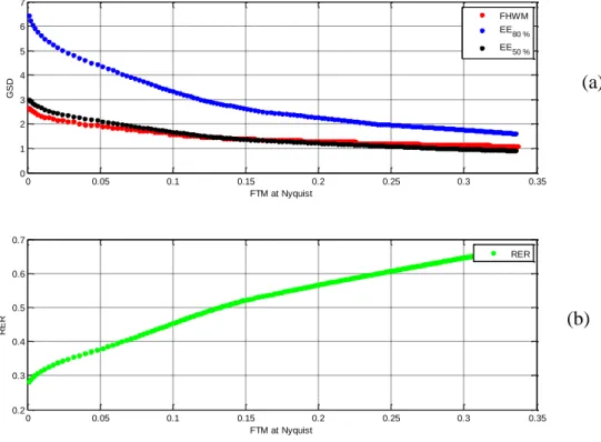
Of course, there are relationships between these different measures as they are related to both PSF and MTF. The EE and FWHM decrease with the MTF value at Nyquist (Figure 1a). On the contrary, the RER is proportional to the inverse of the width of the PSF and increases with the MTF value at Nyquist (Figure 1b).
Figure 1. Example of typical relationship between FWHM, EE diameters (a) and RER (b) with respect to the MTF value at Nyquist.
(a)
(b)
Other spatial resolution-related measures aiming at capturing the complex relationship between resolution performances and parameters related to –or derived from– the MTF, the PSF, the GSD and the SNR. The first example is the general image quality equation (GIQE) proposed by Leachtenauer et al. [22]. This measure takes into account the SNR, RER, GSD, as well as MTF compensation and artifacts in the edge spread function –due to Gibbs overshoots near the edge– to estimate the national imagery interpretability rating scales (NIIRS). This last measure relates directly the quality of an image to the interpretation tasks for which it may be used. Another example is the effective resolution elements (ERE) measure that defines the minimum size of an object with a given contrast within its environment for enabling its detection, location and identification (spatial effective resolution elements or detectable resolution element) or whose radiometric properties can be reliably measured (effective radiometric resolution element) [1, 55].
We give now some definitions about MTF, PSF and their relationships with the line spread function (LSF) and the edge spread function (ESF), as shown in Figure 2. The PSF includes different blur effects, such as optical diffraction and aberrations, detector spatial and temporal integration and motion blur effects. In general case, the PSF is not symmetrical: its Fourier transform, which corresponds to the transfer function of the imagery system, is therefore complex. Its modulus, the MTF, is thus only partial information of the PSF that focuses on Fourier spectral contrast.
The line spread function (LSF) is defined for a given orientation and corresponds to the integration of the PSF over the orthogonal to the direction:
0 0.05 0.1 0.15 0.2 0.25 0.3 0.35 0 1 2 3 4 5 6 7 FTM at Nyquist G S D FHWM EE80 % EE50 % 0 0.05 0.1 0.15 0.2 0.25 0.3 0.35 0.2 0.3 0.4 0.5 0.6 0.7 FTM at Nyquist R E R RER
LSF u PSF u, v dv PSF cos u sin v,sin u cos v dv (1)
Two particular cases of LSF are the horizontal and vertical direction LSF are important because it corresponds to the two separable axes of the detector and the motion blur MTF:
LSF 0 u PSF u, v dv
LSF 2 u PSF v, u dv
(2)
The modulus of the Fourier transform of LSF corresponds to the 1D cross-section of the MTF in the direction :
2i fx
MTF f MTF f cos , f sin LSF x e dx (3)
The edge spread function (ESF) is defined for a given orientation and corresponds to the primitive of the corresponding LSF:
x
ESF x LSF u du (4)
Figure 2. Example of a PSF (a) and the corresponding MTF (d). The line spread function LSF[ for the given direction (b) and the corresponding cross-section MTF[] (e). The edge response function
ESF[ for the direction (c) and the corresponding Fourier transform (f).
3. MTF / PSF in-orbit estimation
3.1. Target based absolute MTF estimation methods
Most of the absolute MTF in-orbit measurement methods for optical spaceborne imagery systems are based on image analysis from acquisition(s) of specific well known targets. Those targets can be
(a) -5 0 5 -5 0 5 -5 0 5 0 0.05 0.1 0.15 GSD (b) -5 0 5 0 0.2 0.4 0.6 0.8 GSD (c) (d) -1 0 1 -1 -0.5 0 0.5 1 0 0.2 0.4 0.6 0.8 1 0 0.2 0.4 0.6 0.8 1 Normalized frequency (e) 0 0.2 0.4 0.6 0.8 1 0 0.2 0.4 0.6 0.8 1 Normalized frequency (f)
dedicated man-made targets such as “on-purpose” painted surfaces [5, 20, 26, 39, 42], specific tarps [17, 38], single or multiple spotlights [25], or even convex mirror array [38]. Those targets can also be, especially for medium and low resolution imagery system, man-made objects such as bridges [15, 46], buildings [20], runway painted lines [5]. Natural objects such as field transitions [21, 26], stars [15] moon border [15], ice shelf [31] are also used as MTF targets.
Those MTF targets can be categorized in four types, as proposed by Léger et al. [26]: The edge targets;
The pulse targets; The impulse targets; The periodic targets. 3.1.1. The edge target
An edge target corresponds to a high dark-bright contrast Heaviside edge. The acquisition of this target by an imagery system enables to obtain an accurate ESF. The derivative of this ESF 1D profile provides an estimation of the 1D cross-section MTF profile on the direction normal to the edge transition. Those targets can be artificial with painted surfaces or specific dark and bright tarps or natural such as agriculture fields, parking lots, ground / building transitions, water / ice shelf transitions or even dark space / moon transitions.
Figure 3. Schematic edge targets.
LW LT LT LT LT LH a Surrounding background
Direction of the MTF profile
Helder et al. [17] give some rules of thumb for an “appropriate” edge target (Figure 3), dedicated to accurate MTF estimation. The target should be large enough to be able to extract an included edge target that is not affected by the surrounding background. The transition distance LT presented in
Figure 3 should be greater than the radius extent of the PSF. They suggest that a raw estimate of this radius is between 3 and 5 times the GSD of the system.
Figure 15 in Appendix A gives an estimation of the radius extent of the PSF, defined as the 95% encircled energy radius, depending on the MTF value at Nyquist. The included “core” target –without the target borders, possibly affected by the surrounding background– should be greater than one extent
radius beyond the edge: the width in the direction of the MTF profile of the target, called LW, should
be greater than twice the radius of the PSF, between 6 to 10 GSD. The height of the target –normal to the MTF profile– should be large enough to “stack” and oversample the ESF in order to respectively improve the SNR budget and increase its sampling frequency. Helder et al. [17] suggest that this height, called LH, should be greater than 20 GSD. The angle of the edge with respect to the direction of
the MTF profile, called a, should be around 90°. A slight difference of a from 90° is important to be able to oversample the ESF. These authors suggest that a difference of 8 degrees from 90° is nearly ideal. Moreover, the dark and bright difference divided by the standard deviation of the noise should be greater than 50.
An edge target corresponds to a high contrast Heaviside edge. The main key parameters of the pulse target are:
the differential radiance L between the dark and bright part of the target; the width of the target in the direction of the MTF profile, noted LW;
the orientation angle a with respect to the direction of the MTF profile; the height LH of the target in the direction normal to the MTF profile.
The image m of an edge target is therefore a set of LH sampled ESFs, in the desired direction of the
MTF profile. Those ESFs correspond to LSFs convoluted by the Heaviside function u. In other words, each line of the image of the edge target is therefore noisy sampled version of the same ESF but slightly translated. This can be written as:
n 0
0
m k ESF k x n / tan n k
LSF u k x n / tan n k (5)
These different versions of “poly-phase” sampled ESF enable the creation of a “synthetic” ESF over-sampled with a factor :
0
m k ESF x k / n k (6)
Where n is an independent Gaussian noise whose standard deviation is noted .
The orientation angle a conditions the maximum over-sampling factor of the ESF along the direction of the MTF profile:
Figure 4. Maximum over-sampling factor depending on the orientation angle with respect to the MTF profile.
There is an important trade-off between the effective chosen oversampling factor and the noise regularization to improve the SNR budget of the reconstructed oversampled profile. Indeed, choosing an oversampling factor less than the maximum one enables to “stack” different sampled ESF noisy profiles for a same sampling phase. In the mean, each sub-sampling of the reconstructed oversampled ESF profile can be seen as the results of the binning of LH real samplings from original noisy sampled ESFs profiles. In other words, this binning improves the SNR budget: the resulting standard deviation of the noise of the stacked and oversampled ESF profile, noted verifies:
n H n
H
L
L (8)
Non-parametric methods different from this “simple” binning are of course available to get regularized oversampled ESF profile from the set of sampled noisy ESFs. Helder et al. [17] proposed a specific filtering method –called modified Savitzky-Golay filter– that is based on parabolic regression on sub-pixel sliding 1-pixel window. In that case, the estimation of the resulting standard deviation of the noise on the oversampled ESF is maybe more complex than the previous equation.
A good compromise is to set the oversampling factor to the smallest value –with an optional margin– enabled by the sampling condition of Shannon, in order to maximize the noise reduction by stacking the LH noisy profiles. Of course, this can be done provided that this “optimal” oversampling
factor is less than the maximum oversampling factor conditioned by the orientation angle a of the target:
opt
min
2
min tan , 1 M arg in
N (9) 60 65 70 75 80 85 90 2 3 4 5 6 7 8 9 10 15 20 a (°) M a x im u m o v e rs a m p lin g f a c to r ma x ( a ) (l o g -s c a le )
Finally, the non-parametric estimation of the LSF from the reconstructed over-sampled ESF profile can be made with the “signal” deconvolution approach developed based on Wiener filtering developed in the Appendix B:
0
m k LSF u x k / n k (10)
The modulus of the Fourier transform of the truncated Heaviside function of width LW and
oversampled by a factor is:
W
sin L f 2
U f L
sin f (11)
For spatial frequencies that are close to odd multiples of the inverse of the edge’s width LW, this
modulus of the Fourier Transform can be approximated by:
W
2k 1 L
f , k , U f
L f (12)
On the contrary, the function U f has zero-crossings for even multiples of 1/ LW and:
W
2k
f , k , U f 0
L (13)
As the width of edge LW is supposed to be large with respect to the PSF’s extent, the alternation
between 0 and L f has a small “frequential period” 1/LW.
Therefore, for suitable frequencies, i.e. in the neighborhood of odd multiples of 1/LW, the relative
root mean square error (rRMSE) of the MTF estimation is:
1 2 2 2 2 MTF W W W 2k 1 L rRMSE f L E H f L L f (14)
The usual approach to estimate the LSF from the ESF reconstructed is the convolution with the first order derivative filter h 1[17, 26]:
1 1 f 0 1 h 1 0 1 2 L i f H f sin 2 f i 2 L L (15)
As shown by the previous equation, this derivative filter approximates the inverse of the Fourier transform of the Heaviside function for small values of spatial frequency. Nevertheless, this filter does not take into account neither the zero-crossings nor the radiometric noise n. Figure 5 represents an example of a Wiener filter compared to the first order derivative filter and to the “strict” inverse filter. The Wiener filter takes into account:
the zero-crossings for even multiples of 1/LW: for those frequencies, the Wiener filter is null;
the standard deviation of the noise: considering this standard deviation with respect to the differential radiance L, the Wiener filter “stops” the deconvolution after the normalized spatial frequency 0.6 and completely damps the signal beyond the normalized spatial frequency 1.
Of course, this is an example: the deconvolution and damping bandwidth of the Wiener filter strongly depends on the SNR of the profile.
Figure 5. Examples of MTFs of the first order derivative filter (green line) and the Wiener filter (blue line). Those transfer functions are compared to the inverse filter of the Heaviside function u (red line).
The resulting relative root mean square errors for these three approaches for the deconvolution of the ESF profile are given in Figure 6. Only odd multiples of 1/LW frequencies have been considered
here. The Wiener approach is obviously the optimal approach and the first order derivative gives the worst results. 0 0.2 0.4 0.6 0.8 1 1.2 1.4 1.6 1.8 2 0 0.01 0.02 0.03 0.04 0.05 0.06 0.07 0.08
Normalized spatial frequency Wiener Filter
H,1 U-1
Figure 6. Examples of relative root mean square errors (in %, in log-scale) for the three different deconvolution kernels (Wiener, first order derivative and inverse kernels) presented in Figure 5.
3.1.2. The Pulse target
A pulse target consists of a bright region surrounded by dark regions (Figure 7). The main key parameters of the pulse target are:
the differential radiance L between the dark and bright parts of the target; the width of the pulse, noted W;
the orientation angle a with respect to the direction of the MTF profile;
the height LH of the target in the direction normal to the MTF profile. The importance of the
orientation angle and the height of the target is exactly the same as for the pulse target presented in the previous sub-section.
Figure 7. Schematic pulse targets.
a LT LT LT LT LW LH W Surrounding background
Direction of the MTF profile
The image m of this target is therefore a set of LH sampled LSFs in the direction of the MTF profile
convoluted by the pulse of width W, noted w. These convoluted LSFs are noted hereinafter LSFw.
0 0.2 0.4 0.6 0.8 1 1.2 1.4 1.6 1.8 2 100 101 102 103 104
Normalized spatial frequency
rR M S EM T F ( % , lo g -s c a le ) Wiener Filter H ,1 U-1
Once the LSFw profile has been computed by stacking and interleaving the different sampling
phases, we obtain a 1D LSFw profile oversampled by the factor with a reduced Gaussian noise n
of standard deviation :
W 0
m k LSF x k / n k (16)
The modulus of Fourier transform of the oversampled pulse target w, noted W verifies, in the
Nyquist interval:
W
sin Wf
f L L W sinc Wf
sin f (17)
Then, applying the equation (58), the relative mean square error of the MTF estimator is, then:
1 2 2 2 2 2 MTF n w L rRMSE f E H f W sin c Wf 1 L (18)
One can note that, on account of the sinc, if the size in pixel W of the pulse target is close to an even number, sinc(Wf) is close to zero in the neighborhood of the Nyquist frequency. The mean square error of the MTF estimator is then close to the expected value of the square of the MTF. It means that, in the case of pulse target’s width close to even multiple of the GSD, the relative root mean square error of the MTF estimator, rRMSEMTF(0.5) at the Nyquist frequency is equal to 100 % !
As an illustration, we have simulated the case of MTF estimation with six pulse targets of different widths (0.2, 0.5, 1, 2, 3 and 5 GSD) with two different ratios L (50 and 200). Figure 8 gives the corresponding relative root mean square error of the MTF estimator in log-scale for different normalized spatial frequencies up to the Nyquist frequency.
This example shows that the accuracy of the MTF estimation for a particular spatial frequency strongly depends on the width of the pulse target. More precisely, on account of zero-crossing of the Fourier transform of the pulse, the relative root mean square error of the MTF estimator is close to 100 % for frequencies in the neighborhood of multiples of the inverse of the width of the pulse. On the contrary, the Fourier transform of the pulse has local maxima for odd multiple of the inverse of twice the width of the pulse. The neighborhoods of those frequencies are therefore the most suitable frequencies for the MTF estimation.
Figure 8. Relative root mean square error of the MTF estimator rRMSEMTF for different widths of
pulse target and for two ratios L LSF (red: 50, blue: 200).
For the same characteristics of the radiometric noise and size of the target LW, a performance
comparison has been made between the edge target and three pulse targets of widths ½ GSD, GSD and 3 GSD (cf. Figure 9a).
The resulting performances for those four targets are presented in Figure 9b. Those performances are formulated in terms of theoretical relative root mean square error of the four different MTF estimations corresponding to the four simulated targets. This figure shows that the performance of the MTF estimation is globally decreasing with the spatial frequency. This performance depends strongly on the width of the targets with respect to the spatial frequency that is considered. For a given SNR and a given target, the relative root mean square error (rRMSE) of the MTF estimation (14, 18) defined for each spatial frequency can be seen as its corresponding SNR function. This SNR function may be exploited in the optimization of the MTF parametric models. For example, in case of optimization based on the root mean square difference between the raw Wiener-based MTF estimation and the modeled one, each term of the sum can be weighted by the inverse of the corresponding value of the SNR function. 0 0.1 0.2 0.3 0.4 0.5 10-1 100 101 102 W = 0.2
Normalized spatial frequency
rR M S EM T F ( % , lo g -s c a le ) 0 0.1 0.2 0.3 0.4 0.5 10-1 100 101 102 W = 0.5
Normalized spatial frequency
rR M S EM T F ( % , lo g -s c a le ) 0 0.1 0.2 0.3 0.4 0.5 10-1 100 101 102 W = 1.0
Normalized spatial frequency
rR M S EM T F ( % , lo g -s c a le ) 0 0.1 0.2 0.3 0.4 0.5 10-1 100 101 102 W = 2.0
Normalized spatial frequency
rR M S EM T F ( % , lo g -s c a le ) 0 0.1 0.2 0.3 0.4 0.5 10-1 100 101 102 W = 3.0
Normalized spatial frequency
rR M S EM T F ( % , lo g -s c a le ) 0 0.1 0.2 0.3 0.4 0.5 10-1 100 101 102 W = 5.0
Normalized spatial frequency
rR M S EM T F ( % , lo g -s c a le )
Figure 9. (a.1) Edge target. (a.2) Pulse target (W = 1/2 GSD). (a.3) Pulse target (W = GSD). (a.4) Pulse target (W = 3 GSD). (b) Resulting relative root mean square error rRMSEMTF(f) for the four
targets (a).
(a) (b)
3.1.3. Other targets : the impulse and periodic targets
An impulse target corresponds to a point source or a set of point sources used to directly obtain an acquisition of the sampled PSF)with one or different sampling grids (spatially or temporally). The artificial targets can be “active” sources such as Xenon lamps or “passive” sources, such as convex mirrors.
The experimental site of ONERA in Faugac-Mauzac (France) has at least two 3 kW Xenon spotlights that can be aimed at spaceborne imagery systems. These artificial impulse targets have been used to assess the absolute MTF of SPOT-5 [25, 26]. Leger et al. draw the conclusion that, on account of the available Xenon lamp power and beam divergence, the GSD of the remote sensing system should be less than 30 m.
Rangaswamy in [38] has tested 1.2 m convex mirrors to create array of artificial passive point sources. This array of point source targets has been used to assess the MTF of Quickbird II (61 cm GSD) and Ikonos (1 m GSD).
Stars can be excellent natural impulse targets provided agile maneuvering satellite platforms. One of the method used to assess the MTF of the Earth Observing-1 Advanced Land Imager (10 m GSD) consisted in scanning different stars by using a slower than nominal angular scan speed [15]. Stars in
0 0.1 0.2 0.3 0.4 0.5 0.6 0.7 0.8 0.9 1 100
101 102
Normalized spatial frequency
rR M S EM T F ( % , lo g -s c a le ) Edge target Pulse Target (W = 0.5) Pulse Target (W = 1) Pulse Target (W = 3) (1) (2) (3 ) (4)
the Pleiades constellation and the star Vega in the Lyrae constellation were found to be excellent natural impulse targets in term of radiance contrast: they have been used to assess the PSF, and therefore the MTF of EO-1 ALI for its different spectral bands.
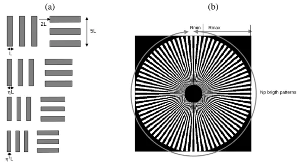
A periodic target consists of specific patterns (edges or pulses) that are periodized. Even if numerical MTF assessment is possible, those targets are in fact meant to direct and quick visually assessment of the resolving power of the imagery system [26]. Examples of those periodic patterns are the standard USAF three-bar pattern or the Siemens radial stars pattern [39] both depicted by Figure 10.
Figure 10. Example of periodic targets: (a) three-bar pattern (typically 6
1 2). (b) Siemens-star pattern. (a) (b) 5L 2L L L L Rmin Rmax Np brigth patterns
The performance analysis of the Wiener approach presented for the edge and pulse targets can be easily derived to be applied for impulse targets and three-bar and Siemens star patterns.
3.2. Bi-resolution MTF estimation methods
The bi-resolution MTF estimation method makes use of ratio of the Fourier spectra of two images of the same scene in order to estimate the ratio of their respective MTF. This approach requires specific pre-processing such as geometric registration and radiometric alignment. Change detection algorithm could be also used to determine areas that are temporally stable between the two instants of acquisition.
This approach can be used for two different cases. In the first case, the two MTF of the two images are unknown and their respective GSD are comparable. In this case, only relative MTF estimation can be done. This approach was used for SPOT systems to estimate temporal evolution of the MTF due to, for example, defocus degradation or spatial MTF variation in the field of view of the instrument [26].
In the second case, one of the two images has a higher spatial resolution by at least a factor 5. In this case, even if the MTF of the high resolution image is unknown, it is assumed to be equal to one, at the scale of the low resolution image. In other words, this approach enables an absolute MTF estimation of the low resolution image. This approach has been used for the SPOT 4 commissioning phase presented by Kubik et al. [21] to assess the MTF of the low resolution sensor Vegetation with the high resolution SPOT image.
A direct approach consists in first estimating the power spectrum density (PSD) of the two co-registred images. These PSD estimations can be achieved by the Welch method [35]. The square root of the ratio of the two PSDs is then an estimation of the ratio of the two MTFs. This “direct” application of the bi-resolution method suffered from an overestimation of the MTF due to aliasing effects [21] [26]. To compensate for these aliasing effects, Viallefont-Robinet [50] proposed a bi-resolution method taking into account PSD estimation of the aliasing component in low bi-resolution image for the MTF estimation.
3.3. “Blind” absolute MTF estimation methods with specific on-board devices
Several specific devices exist aiming at estimating the MTF without any required knowledge of the observed scene or object: in this case, such approaches are called “blind” methods. An example of these “blind” approaches requiring specific on-board devices is the phase diversity method [34]. This image processing technique infers the global MTF from a set of more than two concomitant image acquisitions of the same extended object or “rich” natural scenes (e.g. urban areas).
The first matrix image acquisition corresponds to a “standard” focal-plane acquisition. Therefore, this acquisition takes into account the unknown MTF / PSF.
The other acquisitions are made with additional known perturbations of the MTF. A simple way to do this is to translate the other detector matrixes in the focal plane to induce different known defocuses for the secondary image acquisitions. Practically, the image processing corresponds to a joint and iterative estimation of:
the unknown scene, via a deconvolution processing taking into account of the previous MTF estimation ;
the MTF, via a Zernike model as described in the sub-section §3.4.1, taking into account the current estimation of the unknown object.
Those two conjoint estimations are iterated until convergence. 3.4. Direct and indirect parametric models of the MTF
Different models of MTF exist in the bibliography. Those models can be direct 2D MTF models, or indirectly, through LSF or ESF parametric 1D models. These parametric models can be fitted on the
“raw” MTF / PSF / LSF or ESF estimated by the signal processing approach. There are many optimization approaches to determine those parametric models. The most widely used methods are [37]:
the downhill simplex method: this multidimensional optimization method is useful for non smooth (noisy) or discontinuous cost functions because it does not use the gradient of the cost function to be optimized;
the Levenberg-Marquardt method: this multidimensional optimization method is a gradient and hessian based method. The gradient and the hessian of the cost-function can be given or numerically estimated.
3.4.1. Parametric 2D MTF models
Delvit et al. in [8, 9] have proposed a simplified 2-parameter 2D MTF models:
2
2 2
x y x x x x x y
B C
A
MTF f , f exp f f sinc f sinc f
(19) where fx and fy are spatial frequencies normalized by the sampling frequency, respectively
across-track and along-across-track.
The expression A stands for an approximation of the optical MTF including the diffraction phenomena and different optical errors sources such as aberrations, decentring or focusing. The expression B is an approximation of the detector MTF defined as the MTF degradation due to the spatial integrator effect across-track of the detector. The expression C is an approximation of the detector MTF along-track – sinc(fy) – combined with the smearing along-track effects due to detector
displacement during the integration time.
Léger et al. [25] propose a complementary Steel model in order to take into account more precisely a possible defocus focus of the optical system:
defoc x y 1c x y MTF f , f 2J X f , f (20) where: 2 2 x y x y f , f f f
J1c x J1 x x and J1 is the first order J-Bessel function;
X , f f 1 Nf
N ;
is the central wavelength;
is the detector size (in the focal plane); N is the F-number.
As far as the detector MTF is concerned, a more accurate standard model is a 1 parameter trapezoid detector model:
det det
MTF f sinc f sinc f (21)
To take into account a possible multi-phase Time Delay Integration sub-system (e.g. PLEIADES system) or an integration time less than the line sampling time, the smearing along-track MTF model can be a 1 parameter model:
sm y sm y
MTF f sinc f (22)
Moreover, especially for high resolution system with a “large” time delay integration apparatus, an additional MTF degradation has to be considered. This specific MTF degradation is related to the motion blur due to line of sight temporal perturbations during the integration time. Precise model of motion blur, sometimes called desynchronization MTF for high resolution TDI imagery system such as PLEIADES-HR, can be very complex, depending on the high or low frequency nature of the perturbations with respect to the integration time [45]. The equation below corresponds to a simple model, based upon a low frequency perturbation assumption:
mb mb
MTF f sinc f (23)
The combination of those models, leading to a 7-parameter model, can improve the accuracy and the relevancy of the MTF model by taking into account defocus, motion blur and trapezoidal detector effects on MTF degradation : 2 2 x x x x 1c x y opt x det x det y det y det sm y sm mbx x mby y mb MTF f exp f f 2J X f , f MTF sinc f sinc f MTF sinc f sinc f MTF sinc f MTF sinc f sinc f MTF (24)
It is important to note that the instrument is well known thanks to the detailed optical design and the on-ground calibration of sub-systems such as detectors unit or surface quality mirror (wave front error) that are not prone to change in-orbit. In other words, several parameters have not to be estimated during the in-orbit MTF assessment. Usually, the detector and the smearing along-track MTF degradation are stable and well known. Therefore, their corresponding model parameters have not to be estimated during the in-orbit optimization of the MTF model.
The previous optical MTF model, even with its improvement based on a defocus MTF model, is very simple. Mugnier and Le Besnerais [30] have proposed, for the optical MTF, a « physical » multi-parameter model based on a Zernike orthonormal decomposition of the wave-front error (WFE) that corresponds to the optical aberration in the entrance annular pupil of the instrument:
0
N
l l l l 1
WFE p Z p (25)
where p corresponds to the spatial location in the pupil entrance.
In [30], Mugnier and Le Besnerais have limited the Zernike decomposition to 8 parameters from Z4
(defocus) to Z11 (spherical decomposition).
The optical PSF is then numerically computed as the squared modulus of the Fourier transform of the complex pupil:
x y 2 2i WFE p ,p opt x y x y PSF x, y FT P p , p e , F F (26) where:
x, y corresponds to the spatial location in the focal plane;
P is the pupil support generally circular or even annular, in the case of central obscuration of the telescope;
An intermediate and simpler mean to “physically” model the optical MTF is to combine a perfect diffraction limited optical MTF with a Gaussian global model of optical aberration MTF:
2 2 diff opt x y x y x x y y x y f K F aber opt x y MTF f , f P p , p P p f , p f dp dp F F MTF f , f e (27)
Figure 11 represents cross-sections of the isotropic diffraction limited optical MTF with different ratio of the central obstruction with respect to the pupil diameter.
The two physical previous models have the advantage to be easily “transposed” from a spectral band to another one, by taking into account their respective central wavelengths. Spectral sensitivity
S could be used in those physical models, instead of the central wavelength :
2 2 S diff opt x y x y x x y y x y f K F aber opt x y 1 MTF f , f N S P p , p P p f , p f dp dp d F F MTF f , f N S e d N S d (28)
Figure 11. Cross-section of the diffraction limited optical MTF for different ratios of central obscuration. Frequencies are normalized by the cut-off frequency 1/(N).
3.4.2. Parametric 1D LSF or ESF models
Several models of ESF can be found in the literature that enable to avoid noise and aliasing “contamination” on the MTF cross-section estimation from a edge target. Thomas [47] proposes a sigmoid 3-parameter model:
x 0 1 2
1 ESF x
a a a (29)
Leloglu and Tunali [27] have proposed first a “simple” 3-parameter model based on the error function erf:
0 1 2
ESF x a a erf a x (30)
This model, also mentioned by Helder et al. [17] corresponds in fact to a gaussian model for the PSF, and, therefore, for the MTF. This model is judged in both papers too rough to be able to follow high frequency effects of the ESF, like ringing or ripples near. Indeed, the PSF with its potential skewness and secondary lobes due to diffraction and optical aberrations is definitively not as simple as a Gaussian curve.
To circumvent this limitation, Leloglu and Tunali [27] have proposed a 6-parameter model as a combination with the erf based previous model and a fifth order odd polynomial apodized with a hamming window w: 3 2k 1 0 1 2 l k 1 ESF x a a erf a x w x c x (31)
Helder et al. [17] have mentioned another 10-parameter ESF model based upon Fermi functions, of the form: 0 0.1 0.2 0.3 0.4 0.5 0.6 0.7 0.8 0.9 1 0 0.1 0.2 0.3 0.4 0.5 0.6 0.7 0.8 0.9 1 /D = 0.000 = 0.100 = 0.200 = 0.300 = 0.400 = 0.500
1 3 k k k k 1 x b ESF x d a exp 1 c (32)
In addition to their “intrinsic” model parameters, the different ESF models should have one additional parameter: the sub-pixel shift of the ESF with respect to the sampling grid for the sampled ESF measured in the edge target image.
4. Signal to noise ratio (SNR)
4.1. Definition of the SNR
The signal to noise ratio (SNR) is one of the elements of the image quality. It characterizes the radiometric noise. The image noise quantifies the variation of the radiances at a given radiance level for a uniform landscape. It is defined as:
SNR = m / (33)
where m is the mean of a series of radiances for this uniform landscape and is the standard deviation of this series.
If the imaging system is such that a line of the image is acquired by a CCD array, then the noise in the image is a combination of two separate noises [21, 36]:
column-wise noise, also called instrumental noise: caused by Poisson fluctuation of the signal delivered by the detector and various constant electronic onboard chain noises,
and line-wise noise, also called normalization noise; following image normalization, the residuals may cause visible “columns” on a uniform landscape.
In this case, each noise must be assessed separately. They are then quadratically summed to yield a single value.
If the imaging CCD array is a matrix – e.g., the PolDER system –, then each CCD has its own noise. As there are several normalization steps to equalize the CCDs signal, the noise is assumed in the same way than for the line-wise noise. The SNR is a function of the mean radiance of the landscape. The SNR is usually lower for low values of radiance (dark landscape) because the relative influence of the noise is larger. For large radiances, the SNR increases as the relative influence of the noise decreases. Accordingly, the SNR should be known at different radiance levels.
In some cases, a model can be established that relates the noise to the absolute calibration coefficient, onboard image amplification gain, and radiance. In this way, once the SNR is known for a reference radiance and neutral gain whose value is 1, it can be assessed for any radiance and gain. In the case of a CCD array, the model applies to the column-wise noise [23].
If there is an on-board calibration device, e.g., a calibration lamp, the SNR is estimated by collecting a series of observations of this lamp. This can be done during the planned calibration sequences. The emission of the lamp is assumed to be constant during the period of collection. From this series, the mean and standard-deviation are computed and the SNR is assessed. In case of CCD arrays, this technique can only apply to column-wise noise, i.e., the time-series must be collected by the same CCD [21]. For line-wise noise, vicarious techniques should be adopted.
4.1.1. SNR estimation needs absolute calibration
The SNR is a ratio and its value depends whether it is expressed in radiances or digital counts. The SNR depends upon the quality of the absolute calibration of the instrument and in the case of CCDs array(s) of the inter-CCD and inter-array calibration. The conversion of a digital count DC into radiance L is in the form:
L = a DC + (34)
where a is a gain and an offset.
Because is not zero, the SNR is not equal in digital counts or in radiances. The SNR should be expressed in radiances and it cannot be generally computed with digital counts. The smaller is, the smaller the difference between the two SNRs.
4.1.2. Effects of the atmospheric extinction of radiance on SNR estimation
The radiance measured at system level depends on the optical properties of the atmosphere in both downwards and upwards directions. At first order, and under clear skies, one may write:
Lsat = Lground + Latm (35)
where Lsat is the observed radiance, Lground is the radiance coming from the ground, is the
transmittance of the atmosphere and Latm is the radiance due to scattering by the atmospheric
constituents.
It is usually assumed that the terms and Latm exhibit no high spatial frequencies. Accordingly, the
standard-deviation of Lsat is equal to
[Lsat] = [Lground] (36)
Hereinafter, the operators [ ] and m[ ] denotes respectively the standard deviation and the mean of the operand.
From these equations, one concludes that the SNR differs whether it is computed in radiances with or without atmospheric correction. The lower Latm is, the smaller the difference.
The following is a rough calculation of the error that is committed on the SNR if computed without correction. Let denote SNRsat the SNR assessed from the satellite radiances without correction.
Let SNRactual be the actual SNR. Assuming (36), one obtains a relationship between the SNR assessed
from the satellite and the actual SNR:
ground sat sat ground sat ground sat ground actual m L L m SNR L L m L L L SNR (37) where is equal to atm ground m L L (38)
Assume a typical value of 150 for SNRactual and a value of 0.7 for . Assume that Latm is about 0.05
times m. Then, typically:
11 (39)
This raw calculation indicates the level of uncertainty that can be expected if one does not correct for atmospheric effect. Accordingly, the assessment of SNR should take into account the optical effects of the constituents in the atmosphere.
In addition, this uncertainty may be considered close to that would be observed if the atmospheric terms Latm and contain high frequencies. In [33], Panchev suggested to use the structure function or
variogram –see section 4.5.2– to assess the intensity of the small-scale structures. Practically, it could be applied on images acquired over sites suitable for absolute radiometric calibration of sensors based on the sole observations of the Rayleigh scattering of the light by atmospheric molecules ; this is usually made over the open oceans. During this operation, spatial homogeneity is assumed. Computing the structure function will permit to assess the heterogeneity of these atmospheric terms, though the contributions of the ocean surface may play a role.
4.2. Earth-viewing approach for SNR assessment
Only a very limited number of imaging systems has an on-board calibration device fully appropriate to the assessment of the SNR. Most often, vicarious techniques should be employed. These techniques are based on the earth-viewing approach. In this approach, an image acquired by the system, or combination of images, is used to compute the SNR. The radiance emitted by this landscape has certain properties, e.g., spatial homogeneity, whose knowledge permits to assess the SNR.
Before discussing the methods to assess the SNR in the earth-viewing approach, we should study the role played by the image quality in the assessment of the SNR. As earth-viewing techniques deal
with images, there is a link between SNR, MTF and PSF. The following section shows that a minimum surface exists for an accurate assessment of the SNR.
4.3. Relationships between SNR, MTF and PSF – Minimum surface
The assessment of the MTF has been recognized as depending on the SNR [8, 17, 27]. The MTF assessments are getting noisier as the SNR decreases. In [17], Helder et al. indicate that the SNR should be above 50 for accurate results with edge target methods. Helder and Choi [16] underline that significant tradeoff exists between MTF and SNR.
4.4. Minimum surface for SNR estimation
Reciprocally, it may be shown that the accurate assessment of the SNR is related to the PSF. SNR assessment requires accurate assessments of the standard deviation of the noise. Statistically, for typical remote sensing systems, the assessment of the standard deviation on a homogeneous surface needs a larger number of independent measures than the mean radiance assessment. In other words, the minimum surface of homogeneous regions required for SNR assessment is typically larger than that required for the mean radiance assessment. In the following, we establish a relation between the accuracy of the SNR assessment and the PSF.
The SNR assessment on a homogeneous surface can be viewed as the joint estimation of the mean
m and the variance v 2 of a random Gaussian white noise n. Let us call m ,e ve e2 and SNR e
respectively the estimation of m, v 2 and SNR m v m .
The aim of the following calculation is to determine the minimum number N of independent measures of the random gaussian white noise n to obtain a good accuracy of the SNR assessment. In the remote imagery domain, this minimum number N is related to a minimum homogenous surface of N GSD2.
Let consider nk k 1,N, N independent measures of a random Gaussian white noise n whose mean
m and variance 2
v are both unknown. The unbiased optimal estimators me and ve are, in this case:
N e k k 1 1 m n N and N 2 e k e k 1 1 v n m N 1 (40)
The SNR estimation SNRe is then defined by:
e e e e e m m SNR v (41)
From Student t-distribution TN-1 with N-1 degrees of freedom, the 95 % confidence interval
(noted 95 %-CI) relative error of the mean estimator 0.95m can be derived:
0.025 0.95 N 1 e m N 30 t 2 N m N SNR N (42)
where tN is defined as P TN 1 tN 1 1 where P is the probability density function.
The relative error of the mean estimator depends on the number N of independent measures but also on the SNR. Most spaceborne imagery systems have a SNR greater than, let say, 50. Therefore the relative error of the mean estimator is better than 0.4 % as long as the surface of the homogeneous region exceeds 10x10 pixels.
4.4.2. Relative error of the standard deviation estimator
From 2-distribution with N-1 degrees of freedom, the 95 % confidence interval relative error of the standard deviation 0.95
can be derived: 2 N 1,0.025 0.95 N 1 N (43)
where 2N, is the inverse of the chi-square cumulative distribution function with N degrees of freedom at the values in a.
One can note that the relative error does not depend on the SNR: it only depends on the number N of the independent measures available. Also of interest is the fact that the relative error of the standard deviation estimator is more than 30 times greater than the relative error of the mean estimator for the same surface, for SNR greater than 50. As illustrated in Figure 12, a relative error better than 1 % requires a surface of the homogeneous region greater than 140x140 pixels.
Figure 12. 95 %-CI relative error of the standard deviation estimator versus surface of the homogeneous region in pixel.
4.4.3. Relative error of the SNR estimator
For small mean and standard deviation estimation errors, dm and d, the corresponding SNR estimation relative error dSNR/SNR is given, in first order Taylor expansion, by:
dSNR dm d
SNR m (44)
Therefore, the 95 %-CI relative error of the SNR estimation is approximated by the quadratic sum of the corresponding CI relative errors of the mean and the standard deviation. In other words, for typical spaceborne imagery system (SNR > 50), the 95 %-CI relative error of the SNR estimator is close to the 95 %-CI relative error of the standard deviation estimator. Figure 12 gives the required minimum surface for a given relative SNR accuracy, provided that SNR is greater than 50. However, the SNR assessment should take into account the spatial quality of the imaging system. The extent of the PSF gives the minimum distance between the homogeneous region and the surrounding background to avoid surrounding “contaminations” on the standard deviation assessment.
Consequently, given a relative SNR accuracy, the minimum homogeneous surface for SNR assessment, and more exactly for the assessment of the standard deviation, should obey these two constraints:
LT should be greater than the radius extent of the PSF;
LH x LW should be greater than the required minimum surface.
4.5. Methods to assess the SNR
A method for assessing the SNR is made up of three components that are linked: the selection of the site, the method to compute the mean m and the noise , and the instant when to apply the assessment with respect to routine operations and other calibration operations.
101 102 103 104 105 106
0.1 % 1 % 10 % 100 %
Surface of the homogeneous region in pixel (log-scale)
9 5 % C I R e la ti v e e rr o r o f th e s ta n d a rd d e v ia ti o n e s ti m a to r 0 .9 5 ( % , lo g -s c a le )
There are two approaches in the selection of a site: single view or synthetic landscape. In the single view approach, one image is acquired over a given site. In the synthetic landscape approach, several images are acquired and merged in order to create a synthetic landscape having the requested properties.
4.5.1. Single view – Homogeneous area
The principle of the single view for assessing the SNR is to find a homogeneous area representing a uniform landscape, to compute both the mean and the standard-deviation on this area and finally to build the ratio of the mean to the standard-deviation.
Homogeneous areas have been identified in the world and are used in various calibration operation. However, according to the various publications, it appears that the selection of a large homogeneous area is a problem. There are only a few sites, e.g., Railroad Valley (Nevada, USA) or White Sands (New Mexico, USA), that may be suitable but their spatial homogeneity is not large enough [4, 18, 28, 48].
The influence of the heterogeneity on the SNR assessment depends on the characteristics of the system. What is important are the scales of the heterogeneities with respect to the GSD. For a given intensity in heterogeneity, the larger the GSD, the smaller the influence. The previous section shows that assessing the SNR for a large pixel size requests more ground surface than for a smaller pixel size. Thus, calibration sites may be suitable for certain systems and not for others.
The mean value of the radiance of the landscape should be large enough to obtain a reliable assessment of the SNR. This prevents deep oceanic areas to be exploited to that goal because their reflectivity is low, outside sun glitter conditions.
It appears from the literature survey that selecting a homogeneous area and quantifying its homogeneity is not an easy task. Accordingly, authors have adopted different approaches to cope with this problem of homogeneity. Many of these works intend to select landscapes with no or little high frequencies and to suppress the low frequencies – also called background – in order to obtain a homogeneous landscape.
4.5.2. Single view – Quasi-homogeneous area
One of the most known methods is the Fourier transform of a portion of an image [19, 32]. The noise appears at high wavenumbers (high frequencies). However, the very chaotic behavior of the spectral density for high wavenumbers as well as the presence of large scale trends may render the estimates of both the noise and the mean m rather inaccurate.
A more recent method is to exploit the variogram , also called structure function in turbulence [33]. Because the variance of the noise appears in the variogram as the nugget variance, variogram offer a good readiness of the noise variance even in presence of large variations of the actual signal. It is also invariant, by definition, to systematic errors.
The variogram depicts the spatial variability at increasing distances h (scales) between sample points, as defined by Matheron in [29]:
2
h E Z x h Z x (45)
where E[ ] is the mean operator.
This quantity divided by two is called the semivariogram. The variogram puts on a rational and numerical basis the well-known concept of the "range of influence" of the variable in a fashion more or less similar to the covariance function for a stationary function. Figure 7 illustrates a semivariogram in presence of uncorrelated noise. As the distance h increases, the semivariogram tends to the variance of the image.
Figure 13. Illustration of a semivariogram with uncorrelated noise.
The variogram should equal 0 as h tends to 0. The value of h close to origin gives a measure of the variance of the structures the sizes of which are smaller than the sampling size. This variance 0 is called the nugget effect or nugget variance or random variance.
The spatial behavior of Z(x) is closely related to the shape of (h) near the origin. If (h) is twice differentiable at the origin, then Z(x) is smoothly continuous and it contains rather energetic long wavelength terms. If (h) is linear near the origin, then Z(x) is continuous but not necessarily derivable. lf (h) is not continuous at the origin, hence presenting a nugget effect, Z(x) is not continuous and is rather erratic.
In presence of uncorrelated noise, and if trueh denotes the actual variogram without noise, one
obtains: h = trueh (46) 0 2 4 6 8 10 12 14 16 18 20 0 1 2 3 4 5 6 Distance h V a ri a n c e
The nugget effect is the variance of the noise . If the area is homogeneous, the spatial average of the radiance provides the mean m. If heterogeneous, the image may be locally detrended by adjusting e.g., a polynomial function. The residuals are considered as stationary; the variogram and the average may be computed.
Curran and Dungan [7] and Wald [53] assessed the SNR for respectively AVIRIS and AVHRR images by this means. Outside the difficulties in detrending properly, the issue is the estimation of the unknown (0) from some estimated values of (h). If one assumes that (0) and
hlim0 h are equal, one
may overestimate the variance of the noise. Other approaches, such as extrapolation to ordinate using analytical forms of the semivariogram, may lead to underestimation.
In a recent work [14], Guo and Dou propose a common and feasible way for estimating the variance of the noise, provided a suitable sub-image is found where the signal may be assumed to be stationary; the first application to FY-2 thermal imagery is convincing.
In studies on signal denoising presented in [10], Donoho and Johnston (1994) compute the wavelet coefficients of quasi-homogeneous areas. These wavelet coefficients represent the local intensity of structures for a given scale. Taking the median absolute deviations noted MAD of the finest wavelet coefficients, Donoho and Johnston [10] find that the standard-deviation of the noise can be estimated in a very robust way by:
= MAD / 0.6745 (47)
This method can also be applied in an area exhibiting smooth low frequencies; detrending is nevertheless necessary for the computation of the mean.
More recently, Delvit et al. in [8] exploit both the wavelet transform and the variogram to compute the SNR. They stress the importance of the characterization of the landscape in order to discriminate the landscape information from the noise. They choose to model the semivariogram of an image by the following function:
h = ec hb ea ln(h) (48) where a, b, and c are parameters to be determined, called the landscape structure parameters.
The proposed method is based on an Artificial Neural Network (ANN). The principle is to firstly train the ANN for the noise of simulated or perfectly known images, and then to use the ANN to assess the noise of unknown images. Inputs to the ANN are the landscape structure parameters and elements that characterize the energy in high frequencies.
The authors choose the wavelet packets decomposition, focusing on those packets whose noise is prominent against the landscape signal on account of the damping of the MTF. The MTF induces very important dampening in the diagonals of the Fourier space (Figure 14). For these Fourier areas, the
landscape contribution to the image can be neglected. The entropy and the L² norm of the packet are the inputs to the ANN. This method has also a similar component devoted to the assessment of the MTF; it is quite promising. Its qualities should be demonstrated in real cases. Though, Delvit et al. claim that it should work for any type of landscape, the authors of the present work believe that images exhibiting smooth landscapes with low-energy intrinsic high frequencies would be more suitable for SNR assessment.
Figure 14. Example of adapted wavelet packets decomposition to isolate wavelet coefficients where the MTF is low (source: [8]).
4.5.3. Synthetic landscape
The constraint on a homogeneous existing area may be reduced if one considers a synthetic landscape. A synthetic landscape is constructed by the fusion of actual single images [51]: the properties of the synthetic landscape are more suitable to SNR assessment than those of each single image.
One possible solution is to exploit the existence of desert area whose reflectance is very stable in time, once corrected for bi-directional effects. Such areas were identified by Cosnefroy et al. [6] in Northern Africa. These sites are exploited by Eumetsat for the calibration of the Meteosat satellites [13, 12] , Vegetation [18] and SPOT-5 [23].
If the same pixel is acquired at different cloud-free instants, a time-series of radiances may be constructed which should be constant. The mean and standard-deviation may be computed and the SNR assessed at this radiance level. This approach has not yet been exploited. However, a fairly close approach is used for SPOT-5 by Lebègue et al. [23] for the column-wise noise. Snowy expanses of Greenland in boreal summer and Antarctic in austral summer are assumed to be constant in time, at
least between two consecutive passes. If the two images are perfectly superimposed, the landscape contribution at any scale can be eliminated by a simple difference at each pixel for the area of interest. The residuals are the noise. The standard-deviation is then computed from the residuals, the mean radiance is estimated from the mean of the two images and the SNR can be estimated.
A parameterized model of column-wise SNR function of radiance provides the SNR value at the reference radiance L2: 2 2 0 L SNR L v (49) where:
L is the variance of the photonic noise, proportional to the considered entrance radiance; 2 v is the variance of the readout noise independent of the photonic noise. 0
Another possible solution is to construct this landscape by summing up cloudy images. After a certain period, all pixels are cloudy and under certain conditions, this synthetic landscape may be considered as uniform.
The principle has been discussed by Vermote and Kaufman [49] for absolute calibration. Under certain conditions, radiance reflected by thick clouds exhibits low spatial variance [43, 44]. If one is able to pick-up such cloudy pixels and only those, one may construct a synthetic image of high radiance and low variance. This approach has not been tested for SNR assessment. For past experience, it should be recommended to focus on clouds over deep oceanic areas (e.g., southern hemisphere) to prevent any influence of the ground whose reflectance often exhibits marked spectral changes, and to avoid specular reflection at the surface of the ocean, which is marked by large gradients in reflectance [54].
Such an approach has been applied for performing inter-band calibration of POLDER but for single images [2]. These authors underline that cloud selection is crucial for accurate results and that it depends upon the wavelength under concern. For AVHRR, where the spectral bands are large, the method does not call upon very bright clouds [3]. On the contrary, clouds with medium reflectivity are an ideal target. The method constructs the density of probability of the cloudy pixels and imposes constraints in representation of clouds of medium brightness.
In [24], Lefèvre et al. derived a method for absolute calibration of Meteosat images that was successfully applied by Rigollier et al. [40] for the calibration of several years of images. This method may be applied to the assessment of the SNR.
Lefèvre et al. [24] found two statistical quantities in Meteosat images that are constant with time. They state that this constancy is due to the fact that in the entire field of view of the Meteosat sensor, the mixed presence of land, ocean, and clouds of different reflectivity over approximately one third of
the Earth, whatever the day and time of the year, may lead to the preservation of such statistical quantities with time.
If L5(t) and L80(t) denote respectively the radiances corresponding to the percentiles respectively
5 % and 80 % of the histogram of radiances of the mid-day image, they found that
80 5 0
L t L t
0
t I t (50)
i.e., the quantity (L80(t) – L5(t)) / I0(t) is constant over time, where I0(t) is the incoming extraterrestrial
irradiance. If is the relative eccentricity correction characterizing the change with time in the distance between the sun and the earth, then
I0(t) = I0 (1+) (51)
Using several images, one may construct a time series of this quantity, L5, and L80. Then, one may
compute the mean value m:
80 5
m E L L / 2 (52)
and the noise :
2
80 5
V L L 1 (53)
where V[ ] denotes the operator of variance.
This approach may be applied to sensors having a narrow field-of-view. In that case, several images of e.g., southern oceans with clouds should be summed up to find a constant statistical quantity.
5. Conclusion
We have seen the importance of the parameters MTF and SNR in the assessment of the image quality. The assessments of the MTF and SNR can be performed by the means of respectively specific targets at ground and on-board calibration devices. This review demonstrates that there is a number of algorithms available that permit to exploit suitable landscapes that are found on the earth. It appears that accurate assessment of MTF and SNR can be performed without specific targets and devices. To our opinion, methods are now available and can be operationally implemented for the on-going assessments of the performances in spatial resolution of an optical imaging system aboard a spacecraft. The research in this domain is vivid though limited to space agencies, instruments makers and a few experts in universities. It is benefiting from advances in many scientific domains and especially signal processing and environmental modeling.
Acknowledgements
![Figure 2. Example of a PSF (a) and the corresponding MTF (d). The line spread function LSF[ for the given direction (b) and the corresponding cross-section MTF[] (e)](https://thumb-eu.123doks.com/thumbv2/123doknet/8320123.280426/6.893.97.788.639.1032/figure-example-corresponding-spread-function-direction-corresponding-section.webp)