CROSS SECTION GENERATION STRATEGY FOR HIGH
CONVERSION LIGHT WATER REACTORS
by
BRYAN R. HERMAN
B.S. Nuclear and Mechanical Engineering, 2009 Rensselaer Polytechnic Institute
SUBMITTED TO THE DEPARTMENT OF NUCLEAR SCIENCE AND ENGINEERING
IN PARTIAL FULFILLMENT OF THE REQUIREMENTS FOR THE DEGREE OF MASTER OF SCIENCE IN NUCLEAR SCIENCE AND ENGINEERING
AT THE
MASSACHUSETTS INSTITUTE OF TECHNOLOGY SEPTEMBER 2011
02011 Massachusetts Institute of Technology All rights reserved
Signature of Author.. ...
Department of Nuclear Science
. . .g
*
: . .f .... .- ... Visiting Associate Professor of... and Engineering
July 29, 2011
Eugene Shwageraus, Ph.D. Nuclear Science and Engineering Thesis Supervisor ...
Benoit Forget, Ph.D. Nuclear Science and Engineering
Thesis Supervisor Certified by ... .. .. .. .. Certified by...
y/
Assistant Professor of Certified by ... .. .. .. ... . .. . .. .f. . .. . . . ... . .. . . . Mujid S. Kazimi, Ph.D.TEPCO ofejssor f Nuclear Science and Engineering Professor of Mechanical Engineering Thesis Reader
Mujid S. Kazimi, Ph.D. Chair, Department Committee on Graduate Students
CROSS SECTION GENERATION STRATEGY FOR HIGH CONVERSION LIGHT WATER REACTORS
by
BRYAN R. HERMAN
Submitted to the Department of Nuclear Science and Engineering on July 29, 2011 in Partial Fulfillment of the Requirements for the Degree of Master of Science in Nuclear Science and Engineering
Abstract
High conversion water reactors (HCWR), such as the Resource-renewable Boiling Water Re-actor (RBWR), are being designed with axial heterogeneity of alternating fissile and blanket zones to achieve a conversion ratio of greater than one and assure negative void coefficient of reactivity. This study assesses the generation of few-group macroscopic cross sections for neutron diffusion theory analyses of this type of reactor, in order to enable three-dimensional transient simulations. The goal is to minimize the number of energy groups in these simulations to reduce computational
effort.
A two-dimensional cross section generation methodology using the Monte Carlo code Serpent, similar to the traditional deterministic homogenization methodology, was used to analyze a single RBWR assembly. Results from two energy group and twelve energy group diffusion analyses showed an error in multiplication factor over 1000 pcm with errors in reaction rates between 10 and 60%. Therefore, the traditional approach is not sufficiently accurate. Instead, a three-dimensional homogenization methodology using Serpent was developed to account for neighboring zones in the homogenization process. A Python wrapper, SerpentXS, was developed to perform branch case calculations with Serpent to parametrize few-group parameters as a function of reactor operating conditions and to create a database for interpolation with the nodal diffusion theory code, PARCS. Diffusion analyses using this methodology also showed an error in multiplication factor over 1000 pcm.
The three-dimensional homogenization capability in Serpent allowed for the introduction of ax-ial discontinuity factors in the diffusion theory analysis, needed to preserve Monte Carlo reaction rates and global multiplication factor. A one-dimensional finite-difference multigroup diffusion theory code, developed in MATLAB, was written to investigate the use of axial discontinuity fac-tors for a single RBWR assembly. The application of discontinuity facfac-tors on either side of each axial interface preserved multiplication factor and reaction rate estimates between transport the-ory and diffusion thethe-ory analyses to within statistical uncertainty. Use of this three-dimensional assembly homogenization approach in generating few-group macroscopic cross sections and axial discontinuity factors as a function of operating conditions will help further research in transient diffusion theory simulations of axially heterogeneous reactors.
Thesis Supervisor: Eugene Shwageraus
Title: Visiting Associate Professor of Nuclear Science and Engineering Thesis Supervisor: Benoit Forget
Acknowledgments
I would like to express my sincere appreciation to my advisors, Professor Eugene Shwageraus, Professor Benoit Forget and Professor Mujid Kazimi. The enriching conversations with Professor Shwageraus over the past two years have given me a great understanding of reactor physics and the cross section generation process. I am very thankful that I was able to work and learn from him during his two year visitation at MIT. Professor Forget has provided invaluable insight during the course of this work. He has helped me through many tough problems and gave me new ideas to pursue that have made this work successful. Without Professor Kazimi, this project would not have been possible. I would like to thank him for his guidance.
I would also like to thank Dr. Kord Smith. Without him, the formulation of axial discontinuity factors for this work would not have been possible. I look forward to learning from him as he begins his tenure at MIT.
I would also like to express my sincere gratitude to Dr. Brian Aviles, my fellowship mentor from Knolls Atomic Power Laboratory. He has sparked my interest in multiphysics analyses of nuclear reactors and brought me into the naval lab family. He has been a great source of knowledge during the past few years and I look forward to working with him in the future.
Special thanks to Dr. Jaakko Leppanen for his assistance using the Serpent code. I would also like to thank Professor Downar and his research group at the University of Michigan for their help with PARCS.
Thanks to all of my friends who I have learned so much from over the past few years at MIT and during my undergraduate study at RPI. Our study groups and daily interactions have helped me get through challenging times.
I would also like to thank my closest friends, Robert Gibson and Matthew Mascelli. Their friend-ship and support throughout the years have helped me become the person I am today.
Without my loving family, especially my mother and father, I would not be where I am. They have given me emotional support, encouragement, and financial means as I attain my personal goals. My brother, Christopher, is one of my best friends who is also aspiring to become a nuclear engineer. I dedicate this thesis to him.
This research was performed under appointment to the Rickover Fellowship Program in Nuclear Engineering sponsored by Naval Reactors Division of the U.S. Department of Energy.
Table of Contents
1 Introduction
1.1 Breeding in Light Water Reactors . . . .
1.2 M otivation . . . .
1.3 Homogenization of Cross Sections . . . .
1.3.1 Deterministic Methods -Self Shielding Treatment
1.3.2 Deterministic Methods -Spatial Homogenization
1.3.3 Monte Carlo Methods . . . .
1.4 Full Core Calculations . . . .
1.5 O bjectives . . . .
2 Serpent Reactor Physics Burnup Code
2.1 Using Serpent for Cross Section Generation . . . .
2.1.1 Geometry Creation...
2.1.2 Material Specification . . .
2.1.3 Burnup Calculations .
2.1.4 Detector Tallies . . . .
2.1.5 Other Features . . . .
2.2 Description of Lattice Codes .
2.2.1 Deterministic . . . .
2.2.2 Monte Carlo . . . .
2.3 Two-Dimensional Pin-cell Depletion
2.4 RBWR Serpent Assembly Model .
2.4.1 Geometry Specifications .
2.4.2 Material Specifications . . .
2.4.3 Operating Conditions . . .
2.4.4 Other Control Information .
Comparison . . . . 3 6 . . . 3 8 . . . 3 8 . . . . 3 9 . . . . 4 0 . . . . 4 1 . . . . 4 1 . . . . 4 1 . . . . 4 2 . . . . 4 7 . . . . 4 8 . . . . 4 8 . . . . 5 2 . . . . 5 5 14 14 15 16 16 22 23 31 35 36 36
2.4.5 Comparison with MCNP5 . . . .
2.5 Neutron Balance in Monte Carlo Codes . . . .
2.6 Three-Dimensional Cross Sections . . . .
3 Preparation of Homogenized Parameters
3.1 Branch Cases . . . .
3.1.1 Instantaneous Branch Cases . . . .
3.1.2 History Branch Cases . . . .
3.2 SerpentXS Wrapper . . . .
3.2.1 Input to SerpentXS . . . .
3.2.2 Framework of SerpentXS . . . .
3.2.3 Generation of Homogenized Parameters
3.2.4 Creation of PMAXS Database . . . . .
3.3 Spatial Multigroup Diffusion Solver . . . .
3.4 PWR Lattice Test . . . . 55 57 65 73 . . . 7 3 . . . 74 . . . 77 . . . . 7 9 . . . . 80 . . . . 8 5 . . . . 8 8 . . . . 9 2 . . . . 9 5 .. . . .100
4 Diffusion Theory Analysis of RBWR
4.1 Introduction . . . .
4.2 Two-Zone Examples . . . .
4.2.1 Fissile-Fissile System . . . .
4.2.2 Fissile-Blanket System . . . .
4.3 Axial Discontinuity Factors . . . .
4.3.1 Incorporation of Discontinuity Factors in Finite Difference Equations
4.3.2 Implementation of Discontinuity Factors into Analysis . . . .
4.4 Two-Zone Diffusion Analysis with Discontinuity Factors . . . . 4.5 RBWR Single Assembly Analysis . . . .
4.5.1 Reference Discontinuity Factors . . . .
4.5.2 Application of Discontinuity Factors to PARCS . . . .
107 . . . 107 . . . 107 . . . 108 . . . 108 . . . 115 . . . 116 . . . 118 . . . 121 125 126 . . . 134
4.5.3 Approximation of Discontinuity Factors . . . 136
4.5.4 Effect of Void Distribution on Discontinuity Factors . . . 138
5 Conclusions and Future Work 141 5.1 Conclusions . . . 141 5.2 Future Work . . . 142 5.2.1 Serpent Improvement . . . 143 5.2.2 SerpentXS Improvement . . . 143 5.2.3 Methodology Improvement . . . 144 References 146 A Code Comparison Input Files 150 A. 1 Pin-cell Code Comparisons . . . 150
A.1.1 CASMO4E . . . 150
A.1.2 Dragon . . . 150
A.1.3 BGCORE-MCNP5 . . . 152
A .1.4 Serpent . . . 153
A.2 Serpent -RBWR Single Assembly . . . 155
A.3 MCNP5 -RBWR Single Assembly . . . 168
A.4 RBWR Two-Dimensional Example Input Files . . . 177
A.4.1 Lower Reflector . . . 177
A.4.2 Lower Fissile Zone Sub-region 3 . . . 180
A.4.3 Upper Reflector . . . 183
B SerpentXS -PARCS Input Examples 186 B. 1 SerpentXS Branch Input File . . . 186
B.2 SerpentXS PWR Geometry File . . . 187
C MATLAB Multigroup Spatial Diffusion Solver 193
C.1 Example Input File ... 193
C.2 Source Code . . . 194
C.2.1 Power Iteration Routine . . . 194
C.2.2 Build Loss Matrix . . . 195
C.2.3 Build Production Matrix . . . 198
C.2.4 Fixed External Source . . . 199
C.2.5 Extract Heterogeneous k-effective . . . 199
C.2.6 Compute Interface Currents . . . 200
C.2.7 Coarse Mesh Homogeneous Flux Distribution . . . 201
C.2.8 Compute Homogeneous Interface Flux . . . 202
C.2.9 Extract Heterogeneous Interface Flux . . . 203
C.2.10 Compute Discontinuity Factors . . . 203
D RBWR Single Assembly Code Inputs 205 D .1 Serpent . . . 205
D. 1.1 Branch Case Input File . . . 205
D. 1.2 Geometry Input File . . . 207
D.2 PARCS . . . 219
D.2.1 UF1 PMAXS File . . . 219
List of Figures
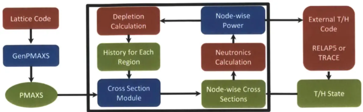
1.1 1.2 1.3 1.4 1.5 1.6 2.1 2.2 2.3 2.4 2.5 2.6 2.7 2.8 2.9 2.10 Side-View of RBWR Assembly Assembly Lattice Configuration Cross-section of a Fuel Rod Unit RBWR Axial Void Fraction Distri Coolant Density Axial Distributio Comparison of Axial Flux Distrib Comparison of Power Density . Comparison of Fission Neutron Pr Comparison of Absorption Rate D Computational Node n NomenclaHitachi Fuel Assembly and Core Layout . . . . Overall Reactor Analysis Calculation Scheme . . . .
Deterministic Cross Section Generation Procedure . . . .
Free-flight Distance in Delta Tracking . . . . PARCS Solution Scheme . . . .
Quarter Core BWR Geometry used in Full Core Analyses . . . . .
Three-Dimensional Homogenization Diagram of a Single Assembly
Pin-cell Geom etry . . . .
Comparison of k-effective for Different Lattice Codes . . . . Difference in k-effective between Several Codes and CASMO4E Comparison of Uranium-235 Number Density versus CASMO4E
Comparison of Plutonium-239 Number Density versus CASMO4E Comparison of Xenon- 135 Number Density versus CASMO4E . .
Dragon -Serpent Comparison of Total Macroscopic Cross Section
Dragon -Serpent Comparison of Fission Neutron Production Cross
S
. . . 4 9 . . . 4 9 C ell . . . 5 1 bution . . . 53 n in RBWR Assembly . . . 57 ution . . . 58 . . . 5 8 oduction Density . . . 59 ensity . . . 59 ture . . . 6 1 2.20 Power Distribution Diagram of RBWR Assembly (side-view) . . . 70
. . . . 15 . . . . 17 . . . . 17 . . . . 25 . . . . 32 . . . . 32 . . . . 37 . . . . 43 . . . . 43 . . . . 44 . . . . 45 . . . . 45 . . . . 46 . . . . 46 ection . . . . 47 2.11 2.12 2.13 2.14 2.15 2.16 2.17 2.18 2.19
2.21 2.22
2.23 3.1 3.2
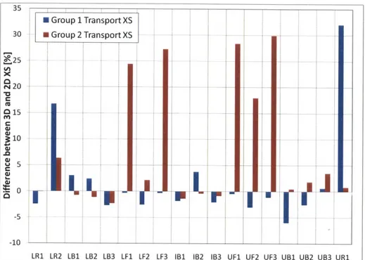
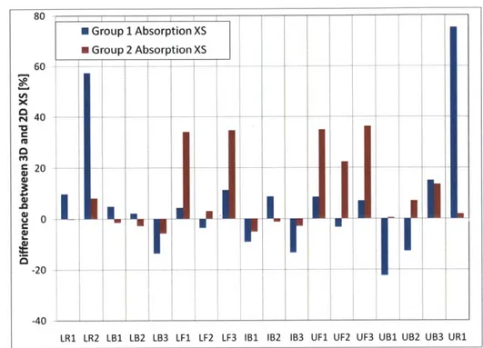
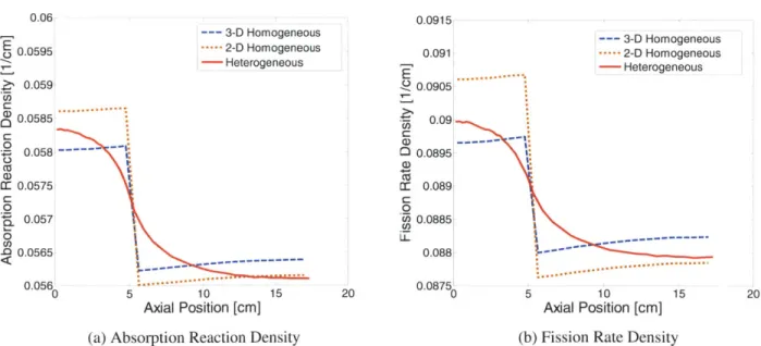
Differences between 3-D and 2-D Transport Cross Differences between 3-D and 2-D Fission Producti Differences between 3-D and 2-D Absorption Cros PMAXS "Tree-Leave" Structure . . . . Fuel Temperature Instantaneous Branch Case PMA
Sectio on Cro
s Secti
XS Ex
3.3 Interpolation Example for History Cases Structure . . . .
3.4 Serpent to PARCS Flow Diagram . . . .
3.5 Overall Flow of SerpentXS Branch Case Generator . . .
3.6 Data Structure Organization in SerpentXS . . . .
3.7 Discretization of Spatial Domain . . . .
3.8 Orientation of Partial Currents at Reactor Boundaries . .
3.9 Homogenization Process of PWR 2-D Lattice . . . .
3.10 Geometry and Power Distribution Pictures from Serpent 3.11 Reference Case Results . . . . 3.12 Control Rod Results . . . . 3.13 Coolant Density Results . . . . 3.14 Poison Concentration Results . . . . 3.15 Fuel Temperature Results . . . .
4.1 Two-zone Homogenization Process . . . .
4.2 4.3
Spatial Distribution of Reaction Densities for the Fissile-F Spatial Distribution of Reaction Densities for Fissile-Blan
4.4 Spatial Flux Distribution for Fissile-Blanket System .
4.5 4.6 4.7 4.8 4.9 ns . . . . 71 ss Sections . . . 71 ons . . . 72 . . . 75 am ple . . . 76 . . . 79 . . . 82 . . . . 86 . . . . 88 . . . . 95 . . . . 98 . . . .101 . . . .102 . . . .104 . . . .104 . . . .105 . . . .105 . . . .106 . . . .109 issile System . . . .109 ket System . . . .113 . . . .113
Spatial Distribution of Reaction Densities for Fissile-Blanket System - 12G Coarse Region Homogeneous Flux Distribution . . . . Comparison of Reaction Densities for Fissile-Blanket System with ADFs . Comparison of Group 1 Collapsed Flux . . . . RBWR Assembly Group I Flux from Two Group Calculation . . . . . . . . 115
. . . . 122
. . . . 122
. . . . 126
4.10 4.11 4.12 4.13 4.14 4.15 4.16 4.17 4.18 4.19 4.20
4.21 Approximated Discontinuity Factors for Two and Twelve Groups . 139
RBWR Assembly Group 2 Flux from Two Group Calculation . . . 129
Assembly Fission Rate Density from Two Group Calculation . . . 131
Fission Production Cross Section from Two Group Calculation . . . 131
Assembly Absorption Rate Density from Two Group Calculation . . . 132
Absorption Cross Section from Two Group Calculation . . . 132
RBWR Assembly Group 3 Flux from Twelve Group Calculation . . . 133
RBWR Assembly Group 12 Flux from Twelve Group Calculation . . . 133
Comparison of Group 3 Absorption Cross Section . . . 134
Assembly Fission Rate Density from Twelve Group Calculation . . . 135
Assembly Absorption Rate Density from Twelve Group Calculation . . . 135
List of Tables
2.1 Geometric and Operating Conditions of Pin-cell . . . 42
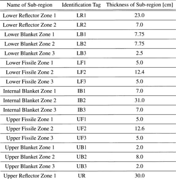
2.2 Description of Sub-Regions in RBWR Assembly . . . 50
2.3 Material Composition of Boron Carbide Rods in LR2 . . . 52
2.4 Material Composition of Depleted UOX in Blanket Regions . . . 52
2.5 Isotopic Composition of TRU Nuclides in Fuel Mixture . . . 53
2.6 Material Composition of Fuel in Fissile Regions . . . 54
2.7 Operating Conditions of RBWR Assembly . . . 56
2.8 Comparison of Eigenvalues between Serpent and MCNP5 . . . 56
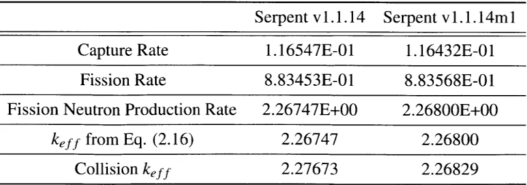
2.9 Comparison of Eigenvalues with Modification of Serpent . . . 65
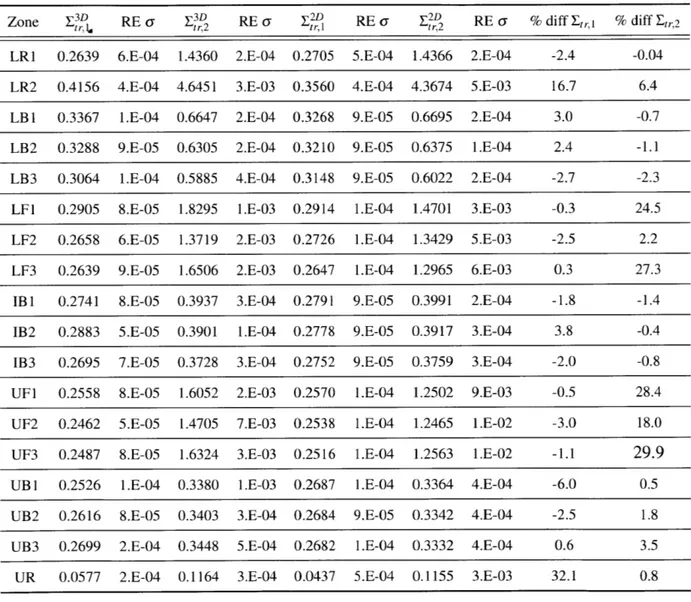
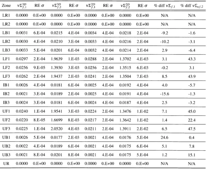
2.10 2-D and 3-D Transport Cross Section Comparison . . . 67
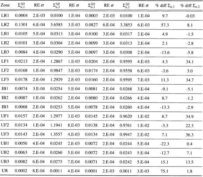
2.11 2-D and 3-D Absorption Cross Section Comparison . . . 68
2.12 2-D and 3-D Neutron Fission Production Cross Section Comparison . . . 69
3.1 Homogenized Parameters for PARCS Calculation . . . 81
3.2 Logicals for PMAXS Database . . . 83
3.3 Parameters for PMAXS File . . . 93
3.4 PWR Geometric Conditions . . . 100
3.5 Instantaneous Branch Case Description . . . 102
4.1 Eigenvalue and Integral Reaction Rates for Fissile-Fissile System . . . 110
4.2 Eigenvalue and Integral Reaction Rates for Fissile-Blanket System . . . 112
4.3 Twelve Group Energy Structure . . . 114
4.4 Eigenvalue and Reaction Rates for Fissile-Blanket System -Twelve Group . . . 114
4.5 Fissile-Blanket Interface Currents for Two Energy Groups . . . 121
4.6 Discontinuity Factors for Different Currents . . . 122
4.7 Current Comparison of Eigenvalue and Reaction Rates . . . 123
4.10 Current Comparison of 12 Group ADF Eigenvalue and Integral Reaction Rates . . 125 4.11 Comparison of Multiplication Factors for RBWR Single Assembly . . . 127 4.12 Reference Two Group Axial Discontinuity Factors . . . 128 4.13 Two Group Discontinuity Factors for Perturbed Void Distribution . . . 140
1 Introduction
1.1
Breeding in Light Water Reactors
A High Conversion Water Reactor (HCWR) or Light Water Breeder Reactor (LWBR) is a nuclear reactor which is cooled by light water and can produce more fissile material than it consumes. The first LWBR program was started by the U.S. Department of Energy in the mid-1960s to develop a light water reactor to expand nuclear fuel resources. This core was designed and built at the Shippingport Atomic Power Station in Shippingport, Pennsylvania and operated for five years. At the end of operation, an examination was completed and concluded that the fissile inventory of the expended core was 1.39 percent greater than the fissile inventory of the initial core (Atherton, 1987).
A breeder reactor produces more fissile fuel than it consumes while it generates energy. A fissile isotope is an isotope that can undergo fission when interacting with thermal neutrons, while fertile isotopes refer to materials that transform into fissile isotopes when interacting with a neu-tron. Each fissile isotope that undergoes fission produces on average two or three more neutrons. One of these neutrons is required for another fission to maintain the nuclear chain reaction, while the others are free to interact or leak from the reactor. To have a high breeding ratio, the remain-ing neutrons need to interact with fertile material to produce more fissile fuel. The conversion or breeding ratio, if it is greater than unity, is defined as the ratio of the average rate of fissile isotope production to the average rate of fissile isotope consumption (Duderstadt and Hamilton, 1976). Some of these neutrons will interact with other non-fuel core materials or eventually leak out of the system. In the Shippingport LWBR, the fissile material was uranium-233 while the fertile ma-terial was thorium-232. After the LWBR program was finished, this style of reactor core was not utilized in the commercial nuclear industry. All of the commercial nuclear reactors in the U.S. are of the Boiling Water Reactor (BWR) or Pressurized Water Reactor (PWR) type.
Two examples of programs in Japan have been established recently to design HCWRs to in-crease utilization of LWR fuel. Hitachi is designing the Resource-renewable Boiling Water Reactor (RBWR) model AC, while the Japanese Atomic Energy Agency is designing the Reduced Mod-eration Water Reactor (RMWR) as part of their innovative water reactor for flexible fuel cycle (FLWR) program (Takeda et al., 2007; Iwarnura et al., 2006; Uchikawa et al., 2007). These reac-tors operate with mixed oxide fuel that has a breeding ratio of 1.01. The core is characterized by two fissile zones sandwiched between axial internal blankets of depleted uranium dioxide (UOX). Unlike conventional BWRs, these advanced reactor designs are axially heterogeneous with fissile zones producing neutrons and blanket zones consuming them. To increase the breeding ratio, these cores must operate at a higher heavy metal to water ratio. This is partially obtained by increasing the void fraction, in some assemblies up to 80%, compared to conventional BWRs. In conventional BWRs, the core average void fraction is about 40%, whereas, in the RBWR it is about 60%. This higher void fraction is obtained by reducing the flow to power ratio. The heavy metal to water ratio is also raised by reducing the pin pitch and arranging it in a hexagonal lattice. An illustration of a fuel assembly and a full core arrangement is shown in Figs. 1. la and 1.1b, respectively. Similar to a conventional BWR assembly, the RBWR fuel assembly has a shroud surrounding it with a control rod inserted between assemblies. The fuel assembly contains five different enrichment fuel pins radially. An assembly of the RBWR contains five distinct active axial core zones: lower blan-ket, lower fissile, internal blanblan-ket, upper fissile and upper blanket. In these type of designs, a high
( 10.7wt% 5
(13.5wt% 22e
( 16.8wt% 51 18.2wt% 70 199.2mm 19.5wt% 123
Average Fissile Pu Enrichment 18.Owt%
Number of Fuel Rods 271
-194.7mm Fuel Rod Diameter 10.1mm
Fuel Rod Gap 1.3mm Thickness of Control Rod 6.5mm
(a) Hexagonal Fuel Assembly Configuration (b) Axial Zone Configuration in Full Core Design
Figure 1.1. Hitachi Fuel Assembly and Core Layout (Takeda et al., 2007)
axial leakage is needed to keep the void coefficient of reactivity negative. Instead of losing these neutrons, they interact in spatially separate blanket zones to produce more fissile isotopes. This axial configuration is shown in Fig. 1. 1b where zones are on top of one another in a parfait form.
A hexagonal assembly that is axially heterogeneous with a high void fraction in the upper part of the assembly, makes it a difficult problem to solve from a reactor physics standpoint. As will be described in Section 1.3, macroscopic few-group cross sections and other parameters required for solution of the neutron diffusion equation are conventionally generated from two-dimensional radial lattice calculations. These cross sections may not be accurate because the RBWR does not have a distinct flux energy spectrum along the third dimension. Rather, this spectrum is con-tinuously changing along the axial direction because of the changing void fraction and material zones. Thus, decoupling zones from each other may not be valid. As the void fraction increases, the moderator in the assembly becomes less dense and the mean free path of neutrons increases. Therefore, neutrons will travel further in the upper portion of the assembly and impact the behavior of neighboring zones. Two-dimensional codes are therefore limited in capturing the effect of such heterogeneity. In this work a Monte Carlo approach is proposed for homogenizing cross sections and other important parameters in this type of core using its three-dimensional neutron transport simulation capability.
1.2
Motivation
The motivation for this work came out of ongoing efforts to perform void coefficient and transient analyses for the RBWR. Since these reactors have a unique axial design, full three-dimensional power/void feedback is required. Before any transient calculations are performed, a steady state solution of the core with a converged power and thermal-hydraulic distribution is needed. The fo-cus of this work is to lay a foundation on how to determine a three-dimensional power distribution of the RBWR. To determine this distribution, a three-dimensional neutronic calculation must be performed which uses few-group homogenized parameters including macroscopic nuclear cross
sections as input. Current conventional two-dimensional homogenization methods do not work for highly heterogeneous cores and therefore a new method is required. The large material discon-tinuities and spectral gradients in the axial direction in these reactors requires a new approach to generating few-group homogenized parameters. This work investigates a three-dimensional ho-mogenization method involving axial discontinuity factors which may be required in generating these few-group homogenized parameters to obtain an accurate full core power distribution.
1.3 Homogenization of Cross Sections
To perform a full analysis of a reactor core, many steps need to be performed to accurately calcu-late the core multiplication factor, reaction rates and lifetime. Although computational power is continuously increasing, the ability for three-dimensional full core transport calculations in rou-tine reactor design is still far in the future. Performing a full core transport calculation would require a solution of a discretized problem of approximately 1012 unknowns. This is unrealistic for routine design, optimization of fuel management and transient calculations. To reduce the compu-tational burden, spatial and energy condensation is performed (Sanchez, 2009). Figure 1.2 shows the general overall process in flow chart form. The process starts with neutron cross section data set preparation from evaluated nuclear data files, then lattice calculations to perform energy and spatial condensation to a few energy groups and ends with a full core reactor calculation.
The neutron cross sections are used to characterize the probability of interactions at different neutron energies. The energy distribution of cross sections is commonly broken up into regions based on important physics that occur in that range. Below about 1 eV is referred to as the thermal energy region where the neutron energy is on the order of the chemical binding energy and thermal motion of molecules of a material. Therefore, it is necessary to take into account the thermal mo-tion of isotopes that are bound in a molecule. Above 1 eV, the resonances of heavy isotopes become important and self-shielding must be taken into account. At this stage, self-shielding is character-ized in terms of an equivalent dilution cross section. Cross sections are parametrcharacter-ized by dilution cross section and by nuclide temperature since the Doppler effect will impact the shape of the res-onances. To perform these steps, a cross section processing code such as NJOY (Macfarlane and Boicourt, 1975) is used. From this point, there are two main methods that will be discussed in order to perform few-group cross section generation: deterministic and stochastic (Monte Carlo). The term few-group cross section generation is equivalent to generation of homogenized parameters or generation of multigroup constants for full core deterministic calculations. In today's industry, deterministic methods are used to generate homogenized few-group cross sections. However, with the increasing computational power, Monte Carlo methods can also be used for this purpose.
1.3.1 Deterministic Methods -Self Shielding Treatment
In nuclear engineering, deterministic methods are classified as methods in which the neutron trans-port equation and/or diffusion equation is discretized and solved directly with numerical methods. An illustration of the steps needed for a deterministic analysis are shown in Figure 1.3. As stated before, the beginning of the process involves processing neutron cross section data. For determin-istic methods, the module GROUPR in NJOY is used to generate a fine structure of multigroup cross sections that are a function of dilution and temperature. Depending on the application, the
Figure 1.2. Overall Reactor Analysis Calculation Scheme (Hebert, 2009)
Basic data base:
- cross-sections
- decay chains energy per Int.
-ission yields
Get basic cross-sections Generate multi-group library Unit-cell Calculations
Fuel Assembly/ Lattice Calculations Whole Core Calculations
Unit cell 1D transport of
equivalent cel
r
a Mato 0 a C31
a a a0 aaC7
a a3 coo 0 a
a ma Do a
0 am 0 am 0
a 00 Mm 0
0 0 moo 0 0
a
C30-Fuel assembty 20 transport or diffusion Reactor coreFigure 1.3. Deterministic Cross Section Generation Procedure Depletionl calculationl
Spitial kinetic", calcul"Itioll
Multigroup cross sections are generated by conserving reaction rates within a specific energy group. To perform this spectral homogenization, GROUPR weights the energy dependent cross section by a flux spectrum as described by
fEg
_1 a, (E') p (E')dE'(ax)g g (1.1)
-1 $(E')dE'
g
In Eq. (1.1), g is the energy group number, (ax), is the group-averaged microscopic cross section for reaction type x, Eg and Eg_1 are the lower and upper boundaries of the energy group,
respec-tively, ax (E) is the energy dependent microscopic cross section for reaction type x and 4 (E) is
the energy dependent flux spectrum. The equation is solvable if both the energy dependent cross section and flux spectrum are known. Unfortunately, the flux spectrum is not known at this step as the full problem would need to be solved in order to know this quantity. In deterministic methods, a flux spectrum must be assumed. Usually, a Maxwellian spectrum is chosen for thermal energy groups, an asymptotic slowing down spectrum is used in the resonance region and a Watt fission spectrum is used in the fast range. The choice of flux spectrum is one of many approximations that must be made in the deterministic methodology.
The fine structure multigroup cross sections are then generated for different dilution cross sec-tions and temperatures. The dilution cross section is also referred to as the background cross section, sigma zero cross section or Bondarenko cross section. This cross section characterizes self-shielding of isotopes and therefore must be generated specifically for isotopes that contain resonances, referred to as resonant isotopes. Cross sections must be generated for a range of di-lution cross sections and temperatures as the didi-lution and temperature of the actual geometry in the full core is not yet known. There are many complicated models for shielding (mutual self-shielding effects) and this is the source of another approximation needed in deterministic methods. The simplest self-shielding method for understanding dilution is the Bondarenko method (Bon-darenko, 1964). For a homogeneous mixture of two materials and isotropic scattering in center-of-mass system, the integral slowing down equation that GROUPR solves is
/E/ai
ES1 (E')Er (E)
#
(E) j ( ,(E')
dE' (1.2)/E/a
2 s2 E' (E') dE'.E (1 - a2) E '
In Eq. (1.2), Et (E) is the energy dependent macroscopic total cross section,
#
(E) is the energydependent scalar neutron flux, Es, (E) is the energy dependent scattering cross section and a, is related to the nuclear mass number (A) for material n,
(A-1
)2. In this example, the subscript nrefers to material numbers where material 1 is the moderator that is a pure scatterer with a constant cross section and material 2 is a purely absorbing resonant isotope such as uranium-238. The macroscopic cross sections can be divided by the number density of the resonant absorber, where the constant cross section of material 1 can be replaced with a dilution cross section, ao. Equation (1.2) becomes
[jO + ar2 (E)]# (E) = f
(E')
dE' (1.3)E (I- 1l) El
/E/a2
Gs2 (E') (E) dEE (I- a2) El
where Ct2 (E) is the energy dependent microscopic total cross section of material 2, Cas2 (E) is the
energy dependent scattering cross section of material 2 and ao is the dilution cross section. In this formulation for a homogeneous system, the dilution cross section is defined as the macroscopic potential scattering (equivalent to total for a pure scatterer) cross section over the number density
of the resonant isotope (material 2),
O - NES (1.4)
N2
Therefore, if the number density of the resonant absorber is small compared to the macroscopic potential scattering cross section of the moderator, the value of the dilution cross section is very
large. In the limit of very small number densities of resonant isotopes, an infinite dilution condition
will exist. This means that the resonances of the resonant absorber are not important in shaping the neutron flux spectrum and therefore the spectrum will take on the asymptotic form of 1/E.
However, if the number density of the resonant absorber is large, the resonances are not diluted
and impact the neutron energy spectrum. In the Bondarenko method, the flux energy spectrum
is represented by the asymptotic form. In the more general case this function can be denoted as
C(E). Therefore the slowing down equation takes on the following form if a narrow resonance approximation is assumed in the moderator (Macfarlane and Boicourt, 1975):
[o + ar2 (E)]
#
(E) C (E) o + 2 s (E) (E') d. (1.5)E (I -- a2) E
For heterogeneous systems, a dilution cross section can also be constructed. According to
equivalence relationships, a heterogeneous system can be represented as a homogeneous system
if the dilution cross sections are equivalent (Duderstadt and Hamilton, 1976). For heterogeneous
systems such as a lattice, the slowing down equation can be constructed in the fuel, where the fuel contains only a pure resonant absorber and the moderator contains a pure scatterer. In addition, it is assumed that rod shadowing is not important such as the case where a single fuel pin is surrounded by an infinite moderator. Thus, once the neutron leaves the fuel pin, it will interact in the moderator.
The slowing down equation can be formulated for this situation in collision probability form,
/E/af
Ef('VfYf (E) Of (E) VfPfaf (E) j( (E') )dE(1.6)
t ~E (I - af) ElO
/E/an
Em (E')+ VmPmng. (E) j ( / ,m (E') dE'.
fE (I -aUm) E
In Eq. (1.6), Vf is the fuel volume, Vm is the moderator volume, Pf f (E) is the energy depen-dent fuel-to-fuel collision probability and Pm>sf (E) is the moderator-to-fuel collision probability.
The subscripts,
f
and m represent the fuel and moderator, respectively. Using the reciprocityre-lation of collision probabilities, Pf-m (E) Ef (E) Vf = Pmsf (E) Em (E) Vm and that neutrons must
be conserved, Pf- + Pf f = 1, Eq. (1.6) can be rewritten as,
VfEt{ (E)
#f
(E) VfPff (E)f
(#
(E')
dE' (1.7)E ( -- af) E'
1 - Pf_ f(E)] Etf(E) Vf E /am Em (E'),
+ Ef (E)
IE
(1 -am) E' OM(E')dE'.The moderator can be assumed to be a pure scatterer and flux energy spectrum in the moderator takes the asymptotic form. The slowing down equation can be written in its final form as
/E/af
E (E') [1 - Pfyf (E)] Ef (E)Ef (E) Of (E) = Pf _f(E) ,f
(E' ) dE'+.
(1.8)t fE 1I - af) Ef E
Using the Wigner rational approximation, the fuel-to-fuel collision probability is Ef (E)
Pf -+f (E) = (1.9)
Eft (E) + Ee
where Ee is a fictitious cross section denoted as the macroscopic escape cross section. The macro-scopic escape cross section is a function of geometry given as the inverse of the mean chord length
of the geometry, 1,
1
Ee . (1.10)
Combining Eqs. (1.8), (1.9) and (1.10), and rearranging it into the form of Eq. (1.5), the dilution cross section (neglecting bell factor, which is a small correction factor for the Wigner rational approximation (H6bert, 2009)) can be identified as
Go = - ==> Ge.(1)
1Nf
Note that C (E) is taken as 1/E in Eq. (1.5). Therefore, for the situation where there is only a purely absorbing resonant isotope in the fuel and lattice effects are neglected, the dilution cross section is the microscopic escape cross section. It is interesting to note that the dilution of the resonant isotope in the fuel for this situation is independent of the moderator. This is because lattice effects were neglected.
To include lattice effects, it is common to characterize the probability that a neutron leaving the fuel will interact with another fuel element. This effect is usually called the Dancoff correction and is commonly denoted as C. The opposite probability is that the neutron interacts in the moderator before colliding in another fuel element and this is known as the Dancoff factor and is denoted as D (Sugimura and Yamamoto, 2006). For the same situation described above, but now taking into account lattice effects, the fuel-to-fuel collision probability is modified to account for rod
Ef(E)
Pf-a_ (E) = (1.12)
Ef (E) +DEe
Therefore, to first order, the dilution cross section is modified yielding
D
GO = Due = - (1.13)
1Nf
In this formulation of the dilution cross section, the moderator dependence is taken into account by the Dancoff factor, where different moderators will yield different Dancoff factors.
A more general situation is when the fuel is made up of both resonant and non-resonant isotopes such as uranium 238 and oxygen. This situation represents a more realistic case where fuel is made up of uranium dioxide. Again, the fuel is arranged in a lattice where lattice effects are taken into account with the Dancoff factor. The slowing down equation for this situation is
/E/af,R
f,R (E')Vf Et(E) Of (E) VfPf f (E) Of (E')dE'
]E (~ - cf,R) E' ()dE
/El/af,NR
Ef,N R E'" V5Pfp g(E) J (F') ,pf (E') dE'
E - af,NR) El
/E/am
Em(E')" VmPm-nf (E)
j
( OM (E') dE', (1.14)fE (1 -- am) El
where the fuel, denoted with superscript
f,
is split into two components: the resonant isotope,denoted with superscript R and non-resonant isotope, denoted with superscript NR. Applying the reciprocity relation, conservation of neutrons and the asymptotic flux energy spectrum for the non-resonant isotope and the moderator, Eq. (1.14) becomes
Ef'R (E) + Ef'NR] Of (E) Pfrf (E) s (F) Pf(E')dE' (1.15)
E (1- af,R) E
Pfa (F) Ef,NR [1 - Pff (E)] Ef'R (E) + Ef'NR
E E
Eq. (1.15) can be rearranged into the form of Eq. (1.5) where C(E) = 1/E. For the definition of the collision probability in Eq. (1.12), the dilution cross section in this form becomes
Ef,NR De(
0 = NR + NR' 1'16)
f f
This form of the dilution cross section can be compared to the heterogeneous form in Eq. (1.13) and the homogeneous dilution cross section in Eq. (1.4). By inspection, the first term in Eq. (1.16) is similar to the homogeneous form and the second term is the heterogeneous form (Yamamoto, 2008). Therefore, the general heterogeneous background cross section is made up of a homoge-neous part and a spatial dependent part. The dilution cross section can be represented in general as
ahet _ hon D2e (1.17)
where the homogeneous background cross section is a superposition of all of the potential cross sections, ay, of non-resonant isotopes (k) in the material,
h Nka k
k f
If the resonant isotopes of the fuel material are not pure absorbers, then the potential scattering
cross section should also be included in Eq. (1. 18).
1.3.2 Deterministic Methods -Spatial Homogenization
After the energy dependence of cross sections has been reduced in the range of hundreds to thou-sands of energy groups, further refinement of the energy groups are made on a pin cell level. As shown in Fig. 1.3, pin cell transport is performed via collision probability methods where a material-specific spectrum can be calculated to account for spatial and energy self-shielding. Since the geometry is starting to be resolved, the dilution of the resonant isotopes can be calcu-lated with Eq. (1.17). The parametrized cross section sets from NJOY can then be interpocalcu-lated
for temperature and dilution so that the appropriate self-shielded cross sections are used in the
transport calculation. Cross sections are then further collapsed into generally tens to hundreds of energy groups. These cross sections are then utilized in lattice calculations (Smith, 1986). For deterministic analyses the lattice calculation involves a two-dimensional slice of an assembly with
zero net current boundary conditions. By assuming zero net current boundary conditions, i.e. no
leakage of neutrons, a distortion in the flux spectrum is present due to deviation from critical con-dition (k-effective of 1). To correct for this, leakage models can be used to force the assembly to yield a multiplication factor that is representative of what would be seen in the actual core.
The geometry is discretized and the the group flux is calculated in every spatial mesh via
col-lision probability methods or method of characteristics (Hebert, 2009). Cross sections are then homogenized spatially over the whole lattice in a few energy groups (Rahnema and McKinley, 2002). The cross sections are homogenized to the point where a full core calculation is feasible in a reasonable amount of time. Before a full core calculation can be performed, cross sections must also be generated for a wide range of possible operating conditions. This process is called generating branch cases and is described in Section 3.1. A description of full core calculations is presented in Section 1.4. The major assumption in deterministic methods at the lattice stage is that the lattice being analyzed can be decoupled both radially and axially from the rest of the core. This approximation has been dealt with by introducing color-sets or supercells, and axial buckling to attempt to capture the spectral effects of neighboring zones. Although this may work for some situations, this assumption may not be applicable in general. The use of Monte Carlo for homog-enized cross section generation may help circumvent many of the needed assumptions that have been discussed for deterministic methods, including the use of equivalent dilution cross section to
1.3.3 Monte Carlo Methods
Although not a new idea, there have been several recent studies using Monte Carlo methods to generate few-group homogenized parameters for full core deterministic calculations (Leppanen, 2007a; Pounders, 2006). In a Monte Carlo analysis, neutrons are simulated one at a time and ran-dom sampling of probability distributions is used to simulate the fundamental physics of neutron transport. The general advantages of using a Monte Carlo code are continuous energy representa-tion of cross secrepresenta-tion data and the ability to handle arbitrary geometry. This is different from the deterministic approach where continuous energy cross sections must be homogenized into a few thousand groups in the first step. A Monte Carlo analysis does not need an initial flux spectrum guess to reduce the number of energy groups. Nuclear cross sections can naturally be defined from the cross section data depending on the neutron's energy. The dilution methodology presented in the deterministic analysis for self-shielding does not need to be performed because continuous energy cross sections are being used in the simulation of neutrons and their interactions. In the resolved resonance region, energy self-shielding is automatically taken into account with a con-tinuous energy representation of resonances. In addition, spatial self-shielding is also captured because neutrons are being tracked individually through the geometry. Dilution cross sections are still needed, however, in the unresolved resonance region where probability tables must be gen-erated (Levitt, 1972). Often in deterministic lattice codes, geometry is restricted because either collision probability or characteristic tracks must be superimposed on the geometry for the analy-sis. If the geometry is restricted to a certain number of configurations, these collision probabilities and characteristic tracks can be optimized to increase computational efficiency. Therefore, it is necessary for these codes to have built-in shapes for geometry. Although these codes can be ex-tended further for odd geometric shapes, it is relatively easy to handle arbitrary geometry in a Monte Carlo analysis. This is due to the simulation of path length of neutrons as they travel from region to region. A drawback of a Monte Carlo method is that it is a statistical process where expected values and associated variances are calculated. In order to get a good estimate of pa-rameters of interest, many particles need to be simulated and this takes computational time. This large computational time factor prevents Monte Carlo methods from being used in routine design calculations for commercial reactors.
Currently, full core Monte Carlo calculations coupled with thermal-hydraulic feedback are very difficult because it would take a prohibitively large amount of time and computing resources. In addition, a Monte Carlo neutronic analysis would also introduce stochasticity to the coupled ther-mal hydraulics analyses when performing both steady state and transient calculations. However, Monte Carlo methods can be used at the lattice level to generate a database of homogenized cross sections for use in full core analyses. Recently, VTT Technical Research Centre of Finland has developed a continuous energy neutron transport code with burnup capability for group constant generation called Serpent (Leppanen, 2007b). Serpent has been benchmarked by comparing re-sults against other neutron transport codes such as MCNP4C and CASMO-4E (Leppanen, 2005). In addition, some experimental benchmarking has been performed against axially-measured fission rates of a VVER-440 (Leppdnen, 2007b). All comparisons and benchmarks yield good results and prove that the physics simulated in Serpent agrees well with established codes and experimental measurements.
Since Serpent was designed specifically for homogenized group constant generation, it requires specialized tallies that are not present in many other codes. One of the limiting factors is that Monte
Carlo codes may take an excessively long time to run to get adequate statistics on these tallies. One method in Serpent that gives it a considerable speed-up is the use of an unionized energy grid for all point-wise cross section data. The main advantage is that the energy grid search needs to be performed only once for each neutron energy. Once the location of this energy point is known, it can be used as an index for each reaction type for all isotopes. Another advantage is that the macroscopic total cross sections can be calculated before the transport cycle, which eliminates the need for this process during the transport cycle. A main drawback of this method is that it requires more memory to store all of these cross section data. This procedure however cannot be done for the unresolved resonance region where the total macroscopic cross section will be determined from the sampling of probability tables. For the other energy regions, this is advantageous because the total cross section is needed to calculate the next flight distance. The free-flight distance that a neutron travels in Monte Carlo is calculated by
In()
s ,(1.19)=
-Et (E, ')
where s is the free-flight distance, 4 is a random number sampled uniformly between 0 and 1, and
Et (E, ') is the precomputed total macroscopic cross section that is energy and material dependent. Finally, another major advantage of a unionized energy grid is that the reactions, dictated by the relative ratio of nuclear cross sections, can be sorted in ascending order. Therefore, when deter-mining a reaction type, the most probable reaction is checked first before all others (Leppanen, 2009).
The other major source of speed-up in Serpent is the use of Woodcock delta tracking (Wood-cock et al., 1965). Delta tracking is an alternative to the conventional surface tracking method that is used to determine the free-flight distance in Eq. (1.19). Since the total cross section in the denominator is a function of material region, it is not statistically valid to sample the neutron across boundaries. Rather, the neutron is moved to the boundary and a new free-flight distance is sampled for the new material region. In the delta tracking method, the material total cross sec-tions are sampled in such a way that the free-flight distances sampled are valid over the entire geometry. To accomplish this, a cross section representing a delta collision is introduced such that the outgoing angle and energy are equivalent to the incoming angle and energy. A virtual total
cross section, E*, (E), can then be calculated as the summation of the material actual total cross
section, Etorm (E) and the delta scattering cross section, ES5m (E),
tot,m (E) = Etot,m (E) + ESm (E). (1.20)
The goal is to determine the smallest value of E,*o,, (E) for each energy such that it is spatially constant, and therefore the delta scattering cross section is allowed to change. Figure 1.4 shows an illustration of how the virtual cross section and total cross section may appear. The value of the virtual cross section corresponds to the maximum total cross section at each energy. Therefore, the free-flight distance can be sampled using the virtual cross section and only one random number is needed. At the collision another random number is sampled to determine if a "true" collision or a delta collision exists. If the delta tracking method is not efficient for the problem being studied, Serpent can use a conventional surface tracking method (Leppdnen, 2010a).
Serpent generates homogenized parameters automatically and lists them in the output file as a function of homogenization region and burnup step. The most important of the parameters
gener-I* XT
S
Figure 1.4. Free-flight Distance in Delta Tracking
ated are the geometry- and group-averaged homogenized cross sections. By simulating neutrons, Serpent is effectively solving Eq. (1.1) in each homogenization region. In Monte Carlo calcula-tions, the neutrons are simulated one at a time and therefore the homogenized cross section is of the form
(EX), = ' .j-~o (1.21)
In Eq. (1.21), (Ex)g is the group and region homogenized macroscopic cross section of reaction x, Exj is the macroscopic cross section that corresponds to the homogenization region and energy group g for the j-th event, and 4j is the flux. In Monte Carlo, there are different estimators of the flux and therefore the j-th event may correspond to a collision or a free-flight travel. Therefore the numerator is just a reaction rate which can easily be determined from built-in tallies that Serpent provides. For all of its tallies, Serpent uses a collision estimator when operating in Delta tracking mode. The collision estimator of the flux (volume integrated and unnormalized) is calculated by
-Wi
# - (1.22)
where wj is the weight of the neutron and Et, is the total macroscopic cross section that corre-sponds to the region and energy group for the j-th event. If Serpent is using surface tracking instead of Delta tracking, it uses a path length estimator of the flux given as
#j
= wjdj, (1.23)where dj is the path length that the neutron travels between collisions. Serpent is an analog Monte Carlo code and therefore the weight of the neutrons is unity and does not change throughout the calculation. Note, in order to get the final estimate of the flux,
#j
in Eqs. (1.22) and (1.23) needs to be divided by total initial source weight and volume of the homogenization region.The homogenization method discussed above works for general macroscopic cross sections needed such as total, absorption, fission and fission neutron production. In addition to these cross sections, a group transfer scattering matrix is also needed to characterize the percentage of neu-trons scattering from one energy group to another. Serpent calculates the probability of a neutron transferring from one group to another by using an analog estimator. It counts how many times a neutron transfers from one energy group to another and normalizes it by the total amount of scattering collisions from each energy group. The group transfer cross section in a certain homog-enization region can then be represented as
Es,h->g - EshPh-+g, (1.24)
where Es,h-g is the macroscopic group transfer scattering cross section between group h and group
g, Es,h is the homogenized macroscopic scattering cross section for energy group h and Phg is the
probability of scattering from group h to group g.
An important parameter to calculate in diffusion theory is the diffusion coefficient. This is probably one of the most difficult parameters to calculate, especially in Monte Carlo. The rigorous definition of the group diffusion coefficient is
Dg9 fVdv 3rf dED(-,E)V# (-r,E)
D =rdE Sfy d3 r
f
dEV 0 (-r, E)(TE) .(1.25)In Eq. (1.25), Dg is the spatial and energy group homogenized diffusion coefficient, D ('r, E) is the diffusion coefficient as a function of space and energy and V# (', E) is the gradient of the space and energy dependent flux (Duderstadt and Hamilton, 1976). This relation is very similar to the definition of a homogenized cross section from Eq. (1.21) except for the gradient of the flux. To get an accurate homogenized diffusion coefficient, the space and energy dependent diffusion co-efficient must be weighted by the current spectrum. Unfortunately, this is very difficult in lattice codes because of the imposition of zero net current boundary conditions. In Serpent, there are two main methods for estimating the diffusion coefficient from flux-weighted homogenized parame-ters. The first definition is derived from the Pi Equations (Bell and Glasstone, 1970), where the group diffusion coefficient can be defined as
1 1
D9 = (1.26)
3Etr,g 3 (Etg - Es1,g)
In Eq. (1.26), Dg is the group diffusion coefficient, Etr g is the macroscopic transport cross section, Et,g is the total macroscopic cross section and Esig is the first moment of the scattering cross section. The first moment of the scattering cross section is defined as the average cosine of the
scattering collision angle,
jo,g,
multiplied by the zeroth moment of the scattering cross section,Eso'g,
Es1,g = Ao19Eso1g. (1.27)
Since neutrons and scattering events are being simulated explicitly, the scattering cosine can be tallied and the average can be taken at the end of the calculation for a specific homogenization re-gion and energy group. Once this parameter is known, the Pi definition of the diffusion coefficient can be calculated.
The next definition of the diffusion coefficient in Serpent is more of a physical interpretation and is derived from the diffusion length. The diffusion length characterizes the distance that the neutron travels before it is absorbed. If this distance is denoted for energy group g by rg, then the mean square distance is related to the diffusion length, Lg, by (Lamarsh, 1966)
= 6L 2 (1.28)
Dg = (1.29)
r1g
where Erg is the removal cross section defined as
Er g = g- Es-,g-+g, (1.30)
The within group scattering cross section, Eslg-,g, represents the probability of a neutron in energy group g undergoing a scattering collision and leaving the collision with an energy also in energy group g. If the homogenization were taking place over one group, the removal cross section would then naturally reduce to the absorption cross section. Eqs. (1.26) and (1.29) were the original def-initions of the diffusion coefficient in Serpent. It was decided that the best diffusion coefficient for multiregion homogenization would be the Pi definition. This is because the mean square distance definition of the diffusion coefficient would correspond to neutrons traveling over multiple homog-enization zones, and therefore would be very difficult to characterize the diffusion coefficient for one of the regions. The Pi definition has more of a local definition and can be applied specifically to a single zone.
The models for diffusion coefficients defined above are different than what deterministic lattice
physics codes use. Current deterministic codes calculate the diffusion coefficient from a B1
fun-damental mode calculation (Stamm'ler and Abbate, 1983). This funfun-damental mode calculation, also called critical spectrum calculation, is important to get a better approximation of the neutron energy spectrum that the geometry will see in the core. Since lattice calculations are performed with zero net current boundary conditions, the system will not be critical and the contribution of neutrons produced from fission will be either overestimated (k > 1) or underestimated (k < 1) (Fridman and Leppanen, 2011). This will inevitably affect the homogenized parameters as they are
weighted by the neutron flux spectrum. The overall goal of the B1 fundamental mode calculation
is to iterate on a buckling term until the multiplication factor is unity. To accomplish this, cross
sections are homogenized over a few thousand groups and used as a starting guess in the B1
equa-tions (Hebert, 2009). The critical flux and current spectrum are then determined from solving the
B1 equations where k-effective is iterated to unity. The cross sections can then be re-homogenized
with the critical spectrum using Eq. (1.21) and the group diffusion coefficients can be calculated from the current spectrum with
Jg
D = (1.31)
where Jg is the group current, B is the buckling and
#g
is the group flux from the critical spectrum. This procedure has been implemented into Serpent and verified for steady state calculations (Frid-man and Leppanen, 2011). Unfortunately, the critical spectrum calculation is not available in the depletion module yet and therefore the Pi definition will be used in this work.The last parameters that are necessary for steady-state multigroup diffusion theory are the group fission spectrum, assembly surface discontinuity factors, assembly corner discontinuity factors and group form functions. The fission spectrum parameter defines the fraction of neutrons that are
emitted from fission into each energy group and is often referred to as the X -spectrum. The group
![Figure 2.5. Figure 2.6.E -10--23Ez4U)4 -5 - ---- -3 0 5 10 15 20 25 30 35 40Burnup [MWD/kgHM]-BGCORE(MCNP5_JEFF3.1) -SerpentENDF/B-VI.8-SerpentENDF/B-Vll.0 -SerpentJEFF-2.2-Serpent JEFF-3.1 -Serpent JEFF-3.1.1](https://thumb-eu.123doks.com/thumbv2/123doknet/14522272.531651/45.918.187.715.139.515/figure-figure-burnup-serpentendf-serpentendf-serpentjeff-serpent-serpent.webp)