Window-Slicing Techniques Extended to Spanning-Event Streams

HAL Id: hal-02947879

https://hal.archives-ouvertes.fr/hal-02947879

Submitted on 24 Sep 2020

HAL is a multi-disciplinary open access

archive for the deposit and dissemination of

sci-entific research documents, whether they are

pub-lished or not. The documents may come from

teaching and research institutions in France or

abroad, or from public or private research centers.

L’archive ouverte pluridisciplinaire HAL, est

destinée au dépôt et à la diffusion de documents

scientifiques de niveau recherche, publiés ou non,

émanant des établissements d’enseignement et de

recherche français ou étrangers, des laboratoires

publics ou privés.

Distributed under a Creative Commons Attribution| 4.0 International License

Streams

Aurélie Suzanne, Guillaume Raschia, José Martinez, Damien Tassetti

To cite this version:

Aurélie Suzanne, Guillaume Raschia, José Martinez, Damien Tassetti. Window-Slicing Techniques

Extended to Spanning-Event Streams. 27th International Symposium on Temporal Representation

and Reasoning (TIME 2020), Sep 2020, Bolzano (virtual), Italy. �10.4230/LIPIcs.TIME.2020.10�.

�hal-02947879�

Spanning-Event Streams

Aurélie Suzanne

Guillaume Raschia

José Martinez

Damien Tassetti

Abstract

Streaming systems often use slices to share computation costs among overlapping windows. However they are limited to instantaneous events where only one point represents the event. Here, we extend streams to events that come with a duration, denoted as spanning events. After a short review of the new constraints ensued by event lifespan in a temporal sliding-window context, we propose a new structure for dealing with slices in such an environment, and prove that our technique is both correct and effective to deal with such spanning events.

2012 ACM Subject Classification Information systems → Stream management

Keywords and phrases Data Stream, Spanning-events, Temporal Aggregates, Sliding Windows

Digital Object Identifier 10.4230/LIPIcs.TIME.2020.10

1

Introduction

Windows have become a pillar of streaming systems. By keeping only the most recent data, they transform infinite flows of data into finite data sets, allowing aggregate functions. These aggregates continuously summarize the data, providing useful insights on the data at a low memory cost. Sliding windows advance across time, and, in many cases, two successive windows share events, leading to redundancy in computation between consecutive or intersecting windows. This redundancy can be avoided. Techniques such as slicing allow to pre-compute aggregates on sub-parts of the windows which can then be shared among several others.

However, these optimisations, and streaming systems in general, were, up to now, limited to instantaneous events only, i.e., points in time (denoted PES). In this paper, we extend streaming systems and their slicing techniques to spanning-event streams (denoted SES) where events are not assigned to a single point in time but rather to a time interval. This extension cannot be done trivially, as lifespan of events imposes a cost on slice computations. Indeed, one spanning event can appear in several slices, which implies that aggregates, such as the count of events, cannot be deduced from the associated slices.

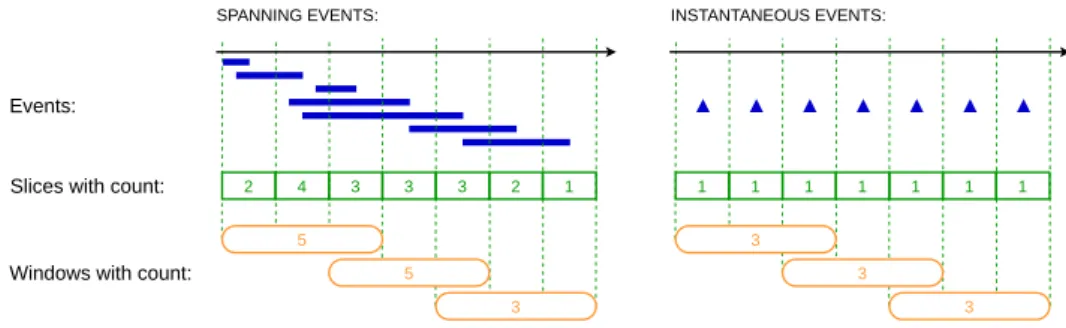
Figure 1 illustrates this problem, the first window contains five events, while the sum of events we can deduce from the associated slices is nine. With point events, both the direct sum of events and the sum from the slices return three.

© Aurélie Suzanne, Guillaume Raschia, José Martinez, and Damien Tassetti; licensed under Creative Commons License CC-BY

27th International Symposium on Temporal Representation and Reasoning (TIME 2020). Editors: Emilio Muñoz-Velasco, Ana Ozaki, and Martin Theobald; Article No. 10; pp. 10:1–10:14

2 4 3 3 3 2 1 Events:

Windows with count:

Slices with count: 1 1 1 1 1 1 1

SPANNING EVENTS: INSTANTANEOUS EVENTS:

3 3 3 5 5 3

Figure 1 Slices and windows with point vs. spanning events.

Applications of these spanning events can be found in particular in monitoring systems dealing with spanning events like telecommunications or transportation. Let us consider a telecommunication network with spanning events like phone calls, and antennas transmitting them. Antenna monitoring consists in retrieving, every five minutes, the number of devices connected to an antenna during the last fifteen minutes. With point events we have either the connection or disconnection of a device to an antenna as an indicator, but cannot use both at the same time. With spanning events we can use the phone call interval, hence improving the accuracy of our metric. In that case, events with device connection, disconnection, or on-going call, can all three be counted correctly as connected to the antenna.

In this paper, we propose a novel slicing technique designed for SES. This technique (1) adapts its structure to aggregate functions, (2) changes the workflow for event insertion to comply with the constraints of event lifespan, and (3) can be plugged into various stream slicer techniques. In order to do so, Section 2 reviews prior work done in the stream optimization field. Then, Section 3 provides background information and extends streams and windows to spanning events. This allows for presenting and extending slice structure to spanning events in Section 4. In Section 5 we study algorithms and complexity which can be achieved with this new structure, and experiment with it in Section 6. We conclude in Section 7.

2

Related Work

Commonly, in a stream, data is processed in an append-only continuous flow of point events which cannot be stored. To compute aggregates on this stream, we need to bound it in time, which allows for finite data set [2]. This is the rationale for windows. Many window flavors exist [5, 14] and this paper focuses on temporal sliding windows. These windows have the particularity to advance with time independently from the stream, using two parameters: the size or range ω, and the step β which determines how fast the window advances in time. Overlaps can happen in such windows as soon as ω > β, e.g., a window of size ω = 15 minutes advancing each β = 5 minutes.

Many techniques have been proposed to improve the performances of sliding windows on PES systems: buffers, buckets, aggregate trees, slices, and their compositions [21]. Naïve techniques keep all the events: buffers do just that, whereas Buckets [12] split them into sets (e.g., one per window). Buckets are especially used for out-of-order processing [13]. With overlapping windows, these methods lead to redundancy in computations as well as to spikes in the system when aggregates are released. Other techniques improve the system efficiency with shared computations among windows. Aggregate trees store partial aggregates in a hierarchical data structure. Slices divide the stream into finite non-overlapping sets of data, keeping only one aggregate value for each slice, on which the final aggregates are then computed. Slices can then be shared among windows. Further applicable optimization techniques depend on the window type used and on the presence of out-of-order events [19, 21].

In this paper, we are particularly interested in slicing techniques for which inner window optimizations can be adapted to spanning events, and their specific constraints. Several methods have been proposed for slices, which differ mainly in the way they create and release slices. Panes [11] provides a first “naïve” implementation, which partitions the stream into constant size slices, equal to gcd(β, ω). This technique generates a high number of slices when the range is not divisible by the step. This led to defining new methods. Pairs [10] creates at most two slices per step. Compared to Panes, this method reduces by a factor of two the number of slices [17]. These two techniques allow to deal with out-of-order streams [22]. Cutty [5] starts new slices at the beginning of windows, and final aggregation executes when needed, without closing any slice, which reduces the number of slices per window by a factor of two compared to Pairs. However, this comes at a cost and reduces effective bandwidth of the stream by sending additional events called punctuation which mark each slice start. As this technique does not separate slices when window ends, it does not allow for out-of-order events [22]. Last but not least, Scotty [22] takes into account out-of-order events with another enrichment of the stream that indicates the start of slices as well as the release of windows, and a system to update slices for which end time has passed when out-of-order events arrive. It also has the specificity of being able to deal with both sliding and session windows, where window bounds are defined by activity and inactivity.

These techniques can be further improved with final aggregation techniques. They define how to merge slice sub-aggregates. Naïve techniques iterate over all the slices (as done in this communication), however this leads to bottlenecks when computing final results. Other techniques compensate this by using aggregate trees or indexes, e.g., B-Int [3], FlatFAT [20], FlatFIT [16], TwoStacks [7], and DABA [18], SlickDeque [17].

3

Preliminaries

3.1

Time, time intervals, and time-interval comparisons

In this paper, we introduce and use time intervals. Time is represented as an infinite, totally ordered, discrete set (T, ≺T), where each time point c is called a chronon [4]. (Discrete) intervals are expressed with a lower and an upper bound, as pairs (`, u) ∈ T × T with

` ≺<sub>T</sub> u. By convention, an interval is written as a left-closed–right-opened interval [`, u).

We denote by I ⊂ T × T the set of time intervals. For any t ∈ I, `(t) ∈ t and u(t) /∈ t are respectively the lower and upper bounds of the interval t. A chronon c can be represented by the interval [c, c + 1).

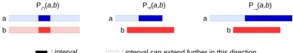
Two intervals can be compared with the thirteen Allen’s predicates [1]. We introduce three new predicates as a combination of Allen’s base predicates, which will prove useful hereafter. They are illustrated in Figure 2. Their corresponding formal definitions are:

P∩(a, b) := `(a) < u(b) ∧ `(b) < u(a), i.e., time intervals a and b have at least one chronon in common;

Pa(a, b) := `(b) < u(a) ≤ u(b), i.e., time interval a ends in b, an asymmetric relation; P→(a, b) := `(a) < u(b) < u(a), i.e., a overlaps and goes beyond b, asymmetric too.

3.2

Spanning-event Stream

Within our SES framework, we consider that each event comes with a time interval, adding the notion of lifespan to events. Instantaneous events can still be modelled with a single-chronon interval. We consider that events are received after their ending.

(a,b)

: interval can extend further in this direction : interval a a b a b b ∩ → P P(a,b) P (a,b)

Figure 2 The three interval comparison predicates used in this paper.

Spanning-event stream (SES) is defined in Equation 1 shown below. Ω corresponds to any set of values, either structured or not, that brings the contents of each event e ∈ S, and

t is the time interval of an event e. We denote by t(e) this value for an event e.

S = (ei)i∈N with ei= (x, t) ∈ Ω × I (1)

The order of events in the stream obeys the constraint: ∀(e, e0) ∈ S2_{, e < e}0 _⇔

u(t(e)) ≺_Tu(t(e0)), which means that events are ordered by their end-time. In this paper, only on-time events are considered. This implies that events are received as soon as their upper bound is reached, at time u(t(e)). The set of streams is denoted by S.

3.3

Aggregate Functions

In streaming systems, data load often makes it impossible to process data individually by an end-user application. A common solution is to use aggregates. Many aggregate functions exist, which can often be studied by categories rather than individually. We use two classifications, based on their properties about slices and spanning events.

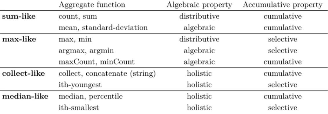
Table 1 presents how common aggregate functions [7, 20] are classified.

One can distinguish several algebraic properties [3, 6, 8, 9, 17] such as: distributive: a stream can be split into sub-streams and some functions allow to compute an aggregate from sub-aggregates, e.g., a sum can be computed from a set of sub-sums; algebraic: an aggregate can be computed from a list of distributive aggregates, e.g., a mean can be computed from sum’s and corresponding count’s sub-aggregates; holistic: some functions do not belong to any of the above categories, e.g., median. No constant bound on storage applies for the last category of functions. This leads to using specifically tailored algorithms. For this reason, this last category is not studied in this paper.

One can also distinguish among accumulative properties [15]: cumulative: an aggreg-ate is an accumulation of all the events, e.g., count adds one for each event; selective: an aggregate keeps only one event, in its original form, e.g., max keeps only the biggest value. Cumulative functions are sensitive to event duplicates. These do happen as a consequence of working with SES. Therefore, we shall study these categories separately.

3.4

Temporal Sliding Window with SES

Windows, in general, allow stream computations by dividing the stream into time intervals of interest where consecutive events can be aggregated. Sliding windows in particular are associated to a time interval. This time interval is defined in advance thanks to two parameters: the range ω, and the step β. Window life-cycle goes through several steps:

window creation is triggered when the window lower bound is reached, and window release is

triggered as soon as the upper bound is reached. Between these two triggers, the window accumulates all the incoming events of interest. At window release, the system computes the aggregate related to this window.

Table 1 Classification of most common aggregate functions.

Aggregate function Algebraic property Accumulative property

sum-like count, sum distributive cumulative

mean, standard-deviation algebraic cumulative

max-like max, min distributive selective

argmax, argmin algebraic selective

maxCount, minCount algebraic cumulative

collect-like collect, concatenate (string) holistic cumulative

ith-youngest holistic selective

median-like median, percentile holistic cumulative

ith-smallest holistic selective

We define such a set of windows in Equation 2. Swi is a finite sub-stream of S containing

the events that occurred in window wi, and ti is the time interval, also denoted t(wi).

WS= (wi)i∈N with wi= (Swi, ti) ∈ S × I (2)

However, SES obliges us to investigate modifications for temporal sliding windows. Firstly, window creation is not impacted by SES as the bounds of the window, t(w), are independent from the stream contents. When a new event arrives, it is assigned to the current window. In contrast, and due to its duration, an incoming event may need to be assigned to past windows too. Thus, triggering a window release at its upper bound would lead to loosing events for this window because they are still on-going and will be known only in the future. To overcome this problem, we introduce a time-to-postpone (TTP). Its role is to delay the window release, with a trigger now happening at the window upper bound plus the TTP. Of course, this value needs to be chosen very carefully as long-standing events could still arrive after the TTP. Several ways exist to define this value, from a fixed user-defined value to an evolving value continuously learned by the system. Accurate definition of the TTP is outside of the scope of this paper, as our topic here is centered on slicing optimizations. Hence we only consider the simplest case of a pre-assigned TTP larger than the largest event expected. With this delay, an event can now be taken into account by any unreleased window. Event affiliation to a window is defined accordingly to the intersection predicate P∩ from Section 3.1.

4

Slices

4.1

Point-event Slices

Slicing techniques divide windows into slices into which events are kept in the form of continuously updated sub-aggregates. These sub-aggregates are then combined in order to compute the window aggregate. Advantages of slices are numerous: (1) they limit memory usage by requiring only one aggregate per slice instead of buffering all the events, and (2) they reduces spikes in the system at window release since only partial aggregates need to be computed, and (3) they allow for computation sharing among windows [5, 11, 22].

We define a sequence of slices in Equation 3. φ ∈ Φ is an internal slice structure that stores the partial aggregate value, and t is the slice interval, also denoted by t(γ). The internal slice structure φ changes depending on the aggregate function used, e.g., sum would keep a sum for each slice, whereas mean would keep a sum and a count. A list of internal

structures for all common aggregate functions can be found in [20].

ΓW,S = (γi)i∈Nwith γi= (φ, t) ∈ Φ × I (3)

Slices obey two properties. They ensure that ΓW,S is a time partitioning of the stream S,

w.r.t. a family window W . These properties are: P1 ∀(i, j) ∈ N2_{, i 6= j → ¬ P}

∩(t(γi), t(γj)): two slices cannot overlap;

P2 u(t(γi)) = `(t(γi+1)): two successive slices meet, in Allen’s meaning.

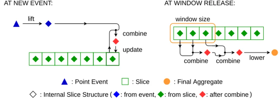
To use our slices, we adopt the incremental aggregation method introduced by Tang-wongsan et al. [20] and re-used in [21]. This approach is based on three functions. They are illustrated in Figure 3, and informally described as follows:

lift : S → Φ transform events for a future insertion in slices. It is used when an event arrives in the system, and transforms it into the internal slice structure.

combine : Φ2_{→ Φ gathers two slices internal structures into a new one. This operation is} used both at event insertion and at window release, as shown in Figure 3.

lower : Φ → Agg: computes the final aggregate from a slice internal structure, in order to actually release a window.

AT NEW EVENT: AT WINDOW RELEASE:

: Point Event lift combine update lower combine combine window size

: Internal Slice Structure

: Final Aggregate : from event, : from slice, : after combine

: Slice

( )

Figure 3 Usage of functions lift, lower and combine to insert events and release aggregates in PES.

As an example, we want to know, every 5 minutes, the number of device disconnections and the maximum call duration for an antenna for the past 15 minutes. For such a query, the slice structure would consist of partial counts and max. An illustrated scenario is as follows: In the initial structure, n represents the partial counts, and max the partial maximums

8 20 19 63 15 19 18 33 14 12 12 47 16 14 time n max 0 5 10 15 20 25 30 35

When a new event with a call duration of 18 minutes arrives at time 34, then: The event is transformed by lift, giving (n = 1, max = 18);

This lifted event is combine’d to the last slice, as illustrated below. 8 20 19 63 15 19 18 33 14 12 12 47 17 18 time n max 0 5 10 15 20 25 30 35

Finally, at window release, we apply two final steps:

We use combine incrementally for the first three slices. A first combine is applied on the two first slices and gives (n = 27, max = 63). Then a second combine on the previous result and third slice results in (n = 42, max = 63).

4.2

Spanning-event Slices

Now, we have to adapt slicing technique to SES. With spanning events, one event can find itself in several slices as shown in Figure 1, which is not the case for point events since slices are non-overlapping. Hence, the first adaptation is to give the possibility to update several slices during the insertion, at the combine level. However, this quickly leads to a duplication problem which we need to leverage. As their sensitivity to duplication varies, we shall study selective and cumulative aggregate functions separately.

4.2.1

Selective Aggregate Functions

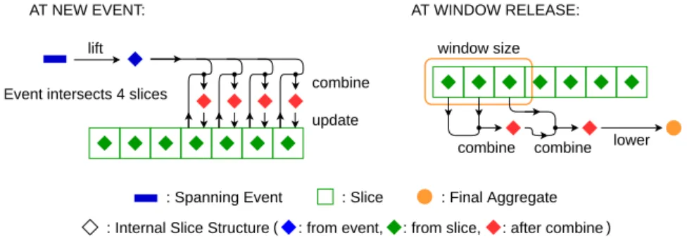
The former is the simpler. With selective functions, e.g., max, duplication of events is not a problem, as only one event is kept. Hence, we can mostly compute selective aggregate functions with the same slice structure used with point-event streams. Figure 4 illustrates the slicing workflow for selective aggregate functions. We can see that only the combine step at event insert-time is modified. Now, all the slices that have a non-empty intersection with

the event need to be updated, not only the last one.

: Internal Slice Structure

AT NEW EVENT: AT WINDOW RELEASE:

lift

combine update

window size

: Spanning Event : Final Aggregate Event intersects 4 slices

: from event, : from slice, : after combine lower combine combine : Slice

( )

Figure 4 Usage of functions lift, lower, and combine to insert events and release aggregates in SES with selective aggregate functions.

Back to our example, we keep the selective function part and compute the maximum call duration with SES as follows:

In the initial structure, the partial maximums are associated to each slice. 20 63 19 33 12 47 14

time 0 5 10 15 20 25 30 35 max

When a new event arrives, say a call duration of 18 minutes at time 34: The event is lift’ed into (18);

This lifted event is combine’d to each related slice, the last four slices here. 20 63 19 33 18 47 18

time 0 5 10 15 20 25 30 35 max

Finally, at window release, we apply the two final steps:

We use combine for the three first slices. This gives (63) after the first combine, next (63) again after the second one.

We apply lower to output a maximum of 63.

4.2.2

Cumulative Aggregate Functions

Cumulative functions accumulate the data, hence they are sensitive to event duplication among slices. To compensate for this problem, we duplicate the internal structure, as shown in Equation 4. We propose the (φ, ϕ)−structure to distinguish between events that end

in the slice, defined with Pa(t(e), t(γ)), from events that follow after the slice, defined by P→(t(e), (t(γ)). To show that our extension performs the expected computations, it is worth to note that P∩ = Pa∨ P→ and Pa∧ P→ = ⊥. In other words, an event that overlaps a given time interval, either finishes inside its time range or goes beyond.

ΓW,S = (γi)i∈Nwith γi= (φ, ϕ, t) ∈ Φ

2

× I (4)

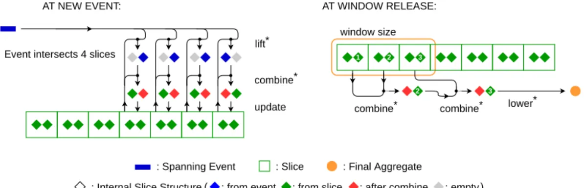
The aggregation process uses modified versions of the lift, combine, and lower operators as described in Section 4.1. This is illustrated in Figure 5. A formal definition of these modified versions is given in Table 2. The new functions operate in the following way:

lift∗_{: S, I → Γ}W,S: classifies each event to the (φ, ϕ) slice structure. To select which part

will be initialized the Pa and P→ conditions are used, resp. for φ and ϕ. Each event is eligible to only one of them, and the non-eligible part is let empty. Basically, as one can see in Figure 5, the last part of the event will contribute to the φ part of the last slice, and to the ϕ part of all other intersecting slices. This implies that the lift∗ operation depends on the interval of the slice, and should be computed for each slice;

combine∗: Γ2W,S → ΓW,S: behaves differently depending on the moment it is triggered.

When combine∗ is triggered at event insertion, it will rely on the raw combine operator from [20] to update as much φ as ϕ. We can however note, as shown in Figure 5, that only one of them will be updated as the event cannot contribute to both at the same time during the lift∗ phase. When combine∗ is triggered at window release it will ignore the ϕ part of the oldest slice to prevent event duplication. We are sure that an event in ϕ will contribute to the next slice, either in φ or ϕ. Hence keeping only the more recent ϕ ensures us neither to duplicate the event nor to forget it. This behavior can be seen in Figure 5 where, at each combine∗, only the ϕ of the most recent slice is kept.

lower∗: ΓW,S→ Agg: merges the distinct parts φ and ϕ to provide the exact aggregate

value.

AT NEW EVENT: AT WINDOW RELEASE:

lift* combine*

update lower*

window size Event intersects 4 slices

2

combine*

3

combine*

: empty : Internal Slice Structure

: Spanning Event : Final Aggregate : from event, : from slice, : after combine,

: Slice

( )

1 2 3

Figure 5 Usage of functions lift∗, lower∗and combine∗to insert events and release aggregates in SES with cumulative aggregate functions. The Internal structure is duplicated to keep track of: the events which end in the slice φ on the left, and the events which end after the slice ϕ on the right.

As neither event duplication nor omission are possible with the (φ, ϕ)−structure we claim that all popular cumulative aggregate functions can be used with this new structure.

We continue our example with the cumulative function part, and use these new functions to count the number of devices connected to an antenna with spanning events.

In the initial structure, φ and ϕ represent partial counts. 8 25 1918 1512 1814 1411 1219 1616 time Φ φ 0 5 10 15 20 25 30 35

When a new event arrive, the phone call with a duration of 18 minutes at time 34: The event is transformed with lift∗into (φ = 1, ϕ = 0) for the most recent slice, whereas it gives (φ = 0, ϕ = 1) for the three previous slices;

This lifted event is combined with each related slice, which are the last four slices. 8 25 1918 1512 1815 1412 1220 1716 time Φ φ 0 5 10 15 20 25 30 35

Finally, at window release, we apply the two final steps:

We use combine∗ for the three first slices. This gives (φ = 27, ϕ = 18) after the first combine∗, then (φ = 42, ϕ = 12) after the second.

We apply lower to output a (correct) count of 54.

Table 2 Extension (∗−form) of slice operators to the (φ, ϕ)−structure for SES. lift∗_{(e : S, t : I) → (φ, ϕ, t) : Γ}W,S lower∗((φ, ϕ, _) : ΓW,S) → y : Agg

φ = lift(e) if Pa(t(e), t) else 0Agg y = lower(combine(φ, ϕ))

ϕ = lift(e) if P→(t(e), t) else 0Agg

combine∗((φa, ϕa, a) : ΓW,S, (φb, ϕb, b) : ΓW,S) → (φ, ϕ, a ∪ b) : ΓW,S

assert u(a) = `(b) or u(b) = `(a) or a = b φ = combine(φa, φb)

ϕ = combine(ϕa, ϕb) if a = b else ϕmax{a,b}

5

Stream Slicer

5.1

Algorithms applicable to SES

We are now able to insert events into slices in order to compute correctly window aggregates from the slices. Next, we need a system able to create such slices from the window parameters and the stream. We saw that for sliding windows several such systems already exist to address PES. However one of our requirements is to be able to update past windows, i.e., windows for which their upper bounds are located in the past. Therefore, in our stream slicer each window end must coincide with a slice end. For this purpose, the algorithms Panes [11] and Pairs [10] are good candidates, while Cutty[5] is unsuitable. However, Panes creates twice as much slices than Pairs. As the goal of a stream slicer is to produce as few slices as possible, in order to reduce insertion and release costs [22], Pairs is more appropriate. Scotty [22] produces slices for each new window start or end, which makes the method equivalent to Pairs. Hence, we shall use the Pairs technique in this paper.

5.2

Slicing Algorithms

For this section we consider cumulative aggregate functions, and each entering event is directly transformed into our aggregate (φ, ϕ)-structure, as defined in Section 4.2.

We use the Pairs technique to separate our input stream into slices. It creates up to two slices per step where the first slice is of size |t(γ₁)| = ω mod β and the second one of size |t(γ₂)| = β − |t(γ₁)|. This leads to nβ= 2 slices per step if ω mod β > 0 else 1, and

Our slice-based SES aggregation process, as exposed in Algorithm 1, uses “an-event-at-a-time” execution model. In this algorithm, one considers τ ∈ T as the clock, i.e., an infinite time counter starting from 0_T. The nωand nβ values are initialized (line 3 - init_nb_slices)

with the above formulas. The tests for the window start and end times (resp. lines 5 and 7) are performed with a T−mark incremented by β each time it is reached. δ corresponds to the TTP and delays window release. read_stream(S, τ ) (line 9) retrieves the event e at current time τ if it exists, or nothing. add_slices in Algorithm 2 creates the missing slices for a new window, the total size of which is β. release_window in Algorithm 3 combines

nωslices, corresponding to all the slices in a window, and then lowers the results to release

a final aggregate. It also deletes the first nβ slices (line 4), to advance the slices structure

in time of a size β. insert_event in Algorithm 4 insert the event in each applicable slice, starting with the more recent, and stopping as soon as it reaches a non intersecting slice.

Algorithm 1 SES Slice Aggregation. input : S ∈ S, ω ∈ N, β ∈ N, δ ∈ N 1 τ : T ← 0_T

2 Γ : List<(Φ, Φ, I)> as Slices ← () 3 nω, nβ: N2← init_nb_slices(ω, β) 4 while True do 5 if window_begins_at(τ ) then 6 add_slices(Γ, τ, ω, β) 7 if window_ends_at(τ − δ) then 8 release_window(Γ, nω, nβ) 9 if e ← read_stream(S, τ ) then 10 insert_event(Γ, e) 11 τ ← τ + 1 Algorithm 2 add_slices. input : Γ ∈ Slices, τ ∈ T, ω ∈ N, β ∈ N 1 if ω mod β > 0 then 2 add (0, 0, [τ, τ + ω mod β[) to Γ 3 add (0, 0, [τ + ω mod β, τ + β[) to Γ Algorithm 3 release_window. input : Γ ∈ Slices, nω∈ N, nβ∈ N 1 γ : (Φ, Φ, I) ← Γ[0] 2 for i ∈ [0, nω[ do 3 γ ← combine∗(γ, Γ[i]) 4 delete slice 0 to nβ−1 from Γ 5 print lower∗(γ)

Algorithm 4 insert_event. input : Γ ∈ Slices, e ∈ S 1 i : N ← | Γ | − 1

2 γ : (Φ, Φ, I) ← ⊥

3 while P∩(t(e), t(Γ[i])) ∧ i ≥ 0 do 4 γ ← combine∗(γ, lift∗(e, t(Γ[i]))) 5 i ← i − 1

5.3

Complexity Analysis

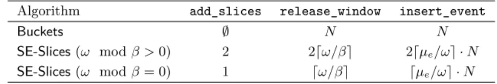
We now compare complexities between the Buckets method and the slicing one. Results are shown in Table 3, for each of the functions given in Algorithms 2, 3 and 4.

The Buckets method allocates one bucket per window. Then, it stores all the N events intersecting a window to its associated bucket. We here store the events in their original form, withtout any pre-aggregation as in the Tuple Buckets technique [21]. The events are hence duplicated for each bucket of every non-closed window they are in. The number of such windows depends on the TTP δ, and is dδ/βe. Then, the aggregate is computed from all the N events in the bucket, only at window release. No sharing can improve complexities in this case.

The slicing technique on the other hand create two slices per step. Initially the cost per window of adding slices is the number of slices per window, 2dω/βe. Nonetheless, because the slices are shared among windows, the cost of adding slices is shared too, one slice being used in dω/βe windows. This leads to a cost of 2 per window for slice addition.

Event insertion in SES has initially a worst case complexity in 2 · O(dω/βe · N ) because all slices could receive all events. However, we assume that most of the time, event size is smaller than the window size. Hence the event needs not be inserted to all slices of a window,

and we prefer to consider the average event size µeto analyze the number of impacted slices.

The complexity becomes then 2 · O(dµe/βe · N ) Again, slice sharing allows us to reduce the

cost, which becomes 2 · O(dµe/ωe · N ) with an upper bound in 2 · O(N ). The best-case

complexity is in O(N/dω/βe) when each event is inserted into only one slice. Hence the behavior of event insertion varies depending on the size of the events.

The final aggregate computation represents the main improvement of our slicing technique, with a complexity depending only on window parameters. The complexity of window release is there reduced from the number N of events to the number 2dω/βe of slices per window, i.e., a constant value.

Finally, we can note that, when ω mod β = 0, only one slice is created per step and all complexities are divided by two (see Table 3).

Table 3 Complexity overview (time cost per window), w.r.t. N , the number of events in a window. Algorithm add_slices release_window insert_event

Buckets ∅ N N

SE-Slices (ω mod β > 0) 2 2dω/βe 2dµe/ωe · N

SE-Slices (ω mod β = 0) 1 dω/βe dµe/ωe · N

The space complexity per window is also greatly improved by the slicing technique. Buckets keeps all then events and hence has a space complexity in O(N ). In contrast, our slicing technique keeps only one pre-aggregate for each slice, with a complexity in O(dω/βe), and only in O(1) when taking slice sharing into account. Notice that if the size is reduced, it also becomes bounded with the slicing technique.

6

Experiments

6.1

Experimental Setup

This series of experiment intends to demonstrate the performance improvements with slices compared to buckets. Throughput in these experiments is achieved by letting the program absorb as many events as it can.

Data Set. We used two data sets. Firstly, a generated data set where each event size is determined by a random number generated with a normal distribution (µ is given as average event size parameter, σ = 10). The system creates a non-delayed stream with one event per chronon, totalling 2M events. Next, the SS7 data set replays a real-world telephony network with one minute of anonymized data containing a stream of 3.2M events. Each event contains 119 fields from which we extract the start and stop times to generate event intervals. δ represents the TTP.

Aggregates. For each window we computed three aggregates: two cumulative functions, namely count and sum, and one selective function, max.

Setup. All experiments were executed on a single core Intel(R) Core(TM) i7-8650U CPU @ 1.90GHz with 16 GB of RAM under Linux Debian 10.

Implementation. Implementation has been coded in modern C++. Algorithms for the slicing method SE-Slices are shown in Section 5.2 for count and sum. max uses a similar algorithm, with a non-duplicated slice structure. For Buckets, we only store event pointers.

6.2

Results

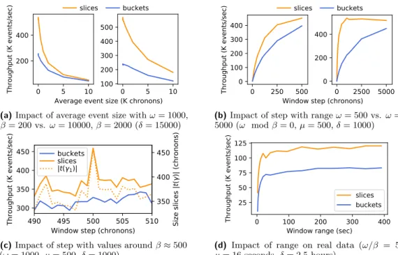
As expected from the complexity review, and as illustrated in Figure 6a, event size has an impact on throughput, for both methods, with SE-Slices performing better than Buckets in all cases. The smaller the event, the best SE-Slices performs. SE-Slices shows an increase in performance for all step sizes when ω mod β = 0 (see Figure 6b). In particular, a significant improvement appears for smaller steps (as long as they are not too close to one), which shows SE-Slices advantage with overlapping windows. When ω mod β > 0, as in Figure 6c, performance improvement is smaller due to the increase in complexity, but slices still perform better than buckets. With real data, and for all window sizes, SE-Slices performs at least 40% better than Buckets (see Figure 6d). In summary, all the experiments show significant improvement in using the slicing technique compared to the bucket one.

0 5 10

Average event size (K chronons) 200 400 Throughput (K events/sec) 100 0 5 10 200 300 400 500 slices buckets

(a) Impact of average event size with ω = 1000, β = 200 vs. ω = 10000, β = 2000 (δ = 15000)

0 250 500

Window step (chronons) 0 100 200 300 400 Throughput (K events/sec) 0 0 2500 5000 200 400 slices buckets

(b) Impact of step with range ω = 500 vs. ω = 5000 (ω mod β = 0, µ = 500, δ = 1000)

490

495

500

505

510

Window step (chronons)

300

350

400

450

Throughput (K events/sec)

350

400

450

Siz

e s

lic

es

|t

(

)|

(ch

ro

no

ns

)

buckets

slices

|t(

)|

(c) Impact of step with values around β ≈ 500 (ω = 1000, µ = 500, δ = 1000)

0 100 200 300 400

Window range (sec) 25 50 75 100 125 Throughput (K events/sec) slices buckets

(d) Impact of range on real data (ω/β = 5, µ = 16 seconds, δ = 2.5 hours)

Figure 6 Throughput metrics comparing slices and bucket techniques.

7

Conclusion

This article extends the problem of aggregate sharing among overlapping windows to

spanning-event streams (SES for short). Dealing with spanning spanning-events brings new constraints, since

events intersect the on-going window as much as past windows. Concerning slicing techniques, dealing with SES implies that adjacent slices can both contain the very same event. Hence, operations sensitive to duplication would provide inaccurate results, and common slicing techniques cannot not be used directly.

Therefore, we extended slicing structures and algorithms depending on the properties of the aggregate functions. When functions are insensitive to event duplicates, we keep the structure and workflow previously used with point events, with a difference however. At event insertion, we update all the intersecting slices instead of only the last one. When functions do have this sensitivity, we duplicate the structure to separate events that ends in the slice from the ones that continue afterwards.

As expected from complexity analyses, slicing techniques with spanning events are computationally more costly than with point events, but they stay, in average, lower than with the buckets technique. Nevertheless, experiments show that the use of slices with spanning events results in significant improvements in throughput. However, when the range is not divisible by the step, performances are only slightly better than with simpler techniques, such as the bucket approach. Hence more advanced techniques need to be experimented in order to circumvent this limiting constraint. Our structure would be of great interest for all techniques which purpose is to partially aggregate spanning events. Eventually, the impact of out-of-order event streams should be studied in our framework.

References

1 James F. Allen. Maintaining knowledge about temporal intervals. Communications of ACM, 26(11):832–843, 1983.

2 Arvind Arasu, Shivnath Babu, and Jennifer Widom. The CQL continuous query language: semantic foundations and query execution. The VLDB Journal, 15(2):121–142, 2006.

3 Arvind Arasu and Jennifer Widom. Resource Sharing in Continuous Sliding-Window Aggreg-ates. VLDB ’04, 30:336–347, 2004.

4 Michael H. Böhlen, Anton Dignös, Johann Gamper, and Christian S. Jensen. Temporal Data Management : An Overview. In eBISS 2017, volume 324, pages 51–83, 2017.

5 Paris Carbone, Jonas Traub, Asterios Katsifodimos, Seif Haridi, and Volker Markl. Cutty: Aggregate Sharing for User-Defined Windows. In CIKM ’16, pages 1201–1210, 2016.

6 Jim Gray, Surajit Chaudhuri, Adam Bosworth, Andrew Layman, Don Reichart, Murali Venkatrao, Frank Pellow, and Hamid Pirahesh. Data Cube : A Relational Aggregation Operator Generalizing Group-By, Cross-Tab, and Sub-Totals. Data Mining and Knowledge

Discovery, 1(1):29–53, 1997.

7 Martin Hirzel, Scott Schneider, and Kanat Tangwongsan. Tutorial: Sliding-Window Aggrega-tion Algorithms. In DEBS ’17, pages 11–14, 2017.

8 Hyeon Gyu Kim and Myoung Ho Kim. A review of window query processing for data streams.

Journal of Computing Science and Engineering, 7(4):220–230, 2013.

9 Sailesh Krishnamurthy, Michael J. Franklin, Jeffrey Davis, Daniel Farina, Pasha Golovko, Alan Li, and Neil Thombre. Continuous analytics over discontinuous streams. In SIGMOD

’10, pages 1081–1092, 2010.

10 Sailesh Krishnamurthy, Chung Wu, and Michael Franklin. On-the-fly sharing for streamed aggregation. In SIGMOD ’06, pages 623–634, 2006.

11 Jin Li, David Maier, Kristin Tufte, Vassilis Papadimos, and Peter A. Tucker. No Pane, No Gain: Efficient Evaluation of Sliding-Window Aggregates over Data Streams. ACM SIGMOD

Record, 34(1):39–44, 2005.

12 Jin Li, Kristin Tufte, David Maier, and Vassilis Papadimos. AdaptWID: An Adaptive, Memory-Efficient Window Aggregation Implementation. IEEE Internet Computing, 12(6):22–29, 2008.

13 Jin Li, Kristin Tufte, Vladislav Shkapenyuk, Vassilis Papadimos, Theodore Johnson, and David Maier. Out-of-order processing: a new architecture for high-performance stream systems.

Proceedings of the VLDB Endowment, 1(1):274–288, 2008.

14 Kostas Patroumpas and Timos Sellis. Window Specification over Data Streams. EDBT ’06, pages 445–464, 2006.

15 Danila Piatov and Sven Helmer. Sweeping-based temporal aggregation. SSTD 2017: Advances

in Spatial and Temporal Databases, LNCS 10411:125–144, 2017.

16 Anatoli U. Shein, Panos K. Chrysanthis, and Alexandros Labrinidis. FlatFIT: Accelerated incremental sliding-window aggregation for real-time analytics. SSDBM ’17, pages 1–12, 2017.

17 Anatoli U. Shein, Panos K. Chrysanthis, and Alexandros Labrinidis. SlickDeque: High Throughput and Low Latency Incremental Sliding-Window Aggregation. EDBT ’18, pages 397–408, 2018.

18 Kanat Tangwongsan, Martin Hirzel, and Scott Schneider. Low-Latency Sliding-Window Aggregation in Worst-Case Constant Time. DEBS ’17, pages 66–77, 2017.

19 Kanat Tangwongsan, Martin Hirzel, and Scott Schneider. Optimal and general out-of-order sliding-window aggregation. Proceedings of the VLDB Endowment, 12(10):1167–1180, 2019.

20 Kanat Tangwongsan, Martin Hirzel, Scott Schneider, and Kun-Lung Wu. General incremental sliding-window aggregation. Proceedings of the VLDB Endowment, 8(7):702–713, 2015.

21 Jonas Traub, Philipp Grulich, Alejandro Rodríguez Cuéllar, Sebastian Breß, Asterios Kat-sifodimos, Tilmann Rabl, and Volker Markl. Efficient Window Aggregation with General Stream Slicing. In EDBT ’19’, pages 97–108, 2019.

22 Jonas Traub, Philipp Marian Grulich, Alejandro Rodriguez Cuellar, Sebastian Bress, Asterios Katsifodimos, Tilmann Rabl, and Volker Markl. Scotty: Efficient Window Aggregation for Out-of-Order Stream Processing. In ICDE ’18’, pages 1300–1303, 2018.