The Effect of Perfect Monitoring of Matched Income on Sales Tax Compliance: An Experimental Investigation

Texte intégral

(1)2008s-17. The Effect of Perfect Monitoring of Matched Income on Sales Tax Compliance: An Experimental Investigation Cathleen Johnson, David Masclet, Claude Montmarquette. Série Scientifique Scientific Series. Montréal Juillet 2008. © 2008 Cathleen Johnson, David Masclet, Claude Montmarquette. Tous droits réservés. All rights reserved. Reproduction partielle permise avec citation du document source, incluant la notice ©. Short sections may be quoted without explicit permission, if full credit, including © notice, is given to the source..

(2) CIRANO Le CIRANO est un organisme sans but lucratif constitué en vertu de la Loi des compagnies du Québec. Le financement de son infrastructure et de ses activités de recherche provient des cotisations de ses organisations-membres, d’une subvention d’infrastructure du Ministère du Développement économique et régional et de la Recherche, de même que des subventions et mandats obtenus par ses équipes de recherche. CIRANO is a private non-profit organization incorporated under the Québec Companies Act. Its infrastructure and research activities are funded through fees paid by member organizations, an infrastructure grant from the Ministère du Développement économique et régional et de la Recherche, and grants and research mandates obtained by its research teams. Les partenaires du CIRANO Partenaire majeur Ministère du Développement économique, de l’Innovation et de l’Exportation Partenaires corporatifs Alcan inc. Banque de développement du Canada Banque du Canada Banque Laurentienne du Canada Banque Nationale du Canada Banque Royale du Canada Banque Scotia Bell Canada BMO Groupe financier Bourse de Montréal Caisse de dépôt et placement du Québec DMR Conseil Fédération des caisses Desjardins du Québec Gaz de France Gaz Métro Hydro-Québec Industrie Canada Investissements PSP Ministère des Finances du Québec Raymond Chabot Grant Thornton State Street Global Advisors Transat A.T. Ville de Montréal Partenaires universitaires École Polytechnique de Montréal HEC Montréal McGill University Université Concordia Université de Montréal Université de Sherbrooke Université du Québec Université du Québec à Montréal Université Laval Le CIRANO collabore avec de nombreux centres et chaires de recherche universitaires dont on peut consulter la liste sur son site web. Les cahiers de la série scientifique (CS) visent à rendre accessibles des résultats de recherche effectuée au CIRANO afin de susciter échanges et commentaires. Ces cahiers sont écrits dans le style des publications scientifiques. Les idées et les opinions émises sont sous l’unique responsabilité des auteurs et ne représentent pas nécessairement les positions du CIRANO ou de ses partenaires. This paper presents research carried out at CIRANO and aims at encouraging discussion and comment. The observations and viewpoints expressed are the sole responsibility of the authors. They do not necessarily represent positions of CIRANO or its partners.. ISSN 1198-8177. Partenaire financier.

(3) The Effect of Perfect Monitoring of Matched Income on * Sales Tax Compliance: An Experimental Investigation Cathleen Johnson†, David Masclet‡, Claude Montmarquette§ Résumé / Abstract Les revenus de plusieurs niveaux de gouvernements sont significativement altérés par la fraude fiscale. Découvrir les déterminants de la fraude fiscale est un défi important alors que ce phénomène pose en même temps la question du design du système de taxation. Combien de ressources devons-nous, par exemple, consacrer à l’audit? Cette recherche mobilisant l’économie expérimentale offre une analyse empirique sur les effets d’assurer systématiquement le contrôle de la taxe de vente et d’étudier les déterminants de s’acquitter du paiement de ce type de taxes. Les résultats indiquent que le contrôle parfait de la taxe de vente sans politiques complémentaires n’augmentent pas nécessairement les rentrées fiscales. Une politique efficace pour réduire la fraude fiscale s’avère une tâche difficile si les agents impliqués ont décidé d’un niveau d’équilibre de conformité dans le paiement de leurs taxes. Les données montrent que les participants tendent à recouvrer leurs pertes suite à un changement de politique fiscale même s’ils doivent prendre plus de risques pour y arriver. Mots clés : taxe de vente, fraude fiscale, économie expérimentale, politiques d’audit. Noncompliance is a quantitatively important phenomenon that affects significantly revenue source for state governments. This phenomenon raises challenging questions about the determinants of tax reporting and also about the appropriate design of a tax system: how many resources should be devoted to auditing? This paper provides specific empirical insights using an experimental approach to measure the effects of systematic sales tax monitoring and the determinants of sales tax compliance. The results indicate that if perfect monitoring is instituted without other complementary policies, an increase in tax revenues is not the likely outcome. A successful policy aiming at reducing fiscal fraud might be a difficult task, once people have decided their equilibrium level of tax compliance. The reference-dependent effect observed in the data suggests that individuals will try to recover their losses following any policy changes even if it means taking more risks. Keywords: sales tax, perfect monitoring, experimental economics, referencedependent effect. Codes JEL : C9, H3, H71 *. The authors thank Nathalie Viennot-Briot for technical assistance. Comments from participants at different seminars were greatly appreciated † University of Arizona. ‡ CREM, CIRANO, Université de Rennes 1. § Université de Montréal, CIRANO, corresponding author: montmarc@cirano.qc.ca..

(4) 1. Introduction Noncompliance is a quantitatively important phenomenon that affects significantly revenue source for state governments. This phenomenon raises challenging questions about the determinants of tax reporting and also about the appropriate design of a tax system: how many resources should be devoted to auditing? There have been a number of studies, theoretical and empirical, on the impact of audits on income compliance.1 Through random surveys (Fisher et al., 1989), and available tax databases (Clotfelter, 1983; Dubin et al, 1990; Erard and Ho 2001), researchers have identified characteristics of noncompliant taxpayers and what is likely to motivate tax compliance. Clotfelter (1983) was the first to provide an empirical analysis of taxpayer compliance with information from the Taxpayer Compliance Measurement Program (TCMP) of the Internal Revenue Service in the United States. He concluded that non-compliance is strongly related to the marginal tax rate. Dubin et al (1990) investigated the impact of audit rates and tax rates on tax compliance with state-level time series from 1977 to 1985. The authors observed that the continual decline in the audit rate over this period led to a significant decrease in IRS collections. Many studies have been done on fraud and tax evasion that use the experimental economics approach concerning, for example, audit rates, penalties and tax compliance with earned versus endowed incomes (see Webley et al 1991, Alm et al 1992a, Boylan and Sprinkle 2001, Gërxhani and Schram, 2006, and Cadsby et al, 2006). Most studies on compliance have focused on personal income tax. Despite the importance of the sales tax in state finances, surprisingly little academic research has focused on the subject of sales tax compliance with some exceptions (Mikesell 1985, Murray 1995, Alm et al 2004). If in general, both the magnitude and determinants of sales tax noncompliance remain elusive targets, Murray (1995) has. 1. See Jackson and Milliron (1986), Roth and Scholtz (1989), Slemrod (1992), Andreoni et al. (1998).. 1.

(5) shown that taxpayers with greater opportunities to reduce their tax liabilities exploit these opportunities to their advantage. He also concluded that there is no obvious nor easy-to-implement policy to combat sales tax noncompliance. The purpose of this paper is to provide specific empirical insights using an experimental approach to measure the effects of systematic sales tax monitoring and the determinants of sales tax compliance. The experimental approach makes it possible to measure exactly the rate of tax compliance. We investigate to what extent taxpayers would alter their compliance behavior in response to a change in the audit occurrence. In particular, we study if perfect monitoring through electronic payment of matched sales income may improve tax compliance and raise the level of tax revenues. Perfect monitoring of sales income is identical to increasing the audit rate on matched income to 100%. It is technically possible if not prohibitively expensive to match individual declaration of income to relevant third party information. In the US, this type of matching is reserved for audits and taxpayer compliance studies.2 The Canadian federal government matches random individual tax returns with third party information on earnings as part of an ongoing monitoring system of tax compliance.3 4 The main objective in instituting direct and automatic capture of sales taxes through electronic payments is to increase revenues by reducing tax evasion. Information reporting on matched income severely limits an individual’s ability to evade taxes. For instance, higher detection probabilities reduce the marginal benefit of evasion and therefore make evasion less attractive. For example, in the US, small businesses and farms, which have less income reporting from third party, have significantly higher rates of evasion. In France, it is estimated that 25% of the fiscal fraud over the 1988-1992 period. 2. Internal Revenue Service (1996). Canada Revenue Agency, source: http://www.cra-arc.gc.ca/tax/individuals/topics/income-tax/reviews/menu-e.html 4 At present, financial institutions credit electronic purchases (including the levied taxes) to the merchant within 24 hours following the purchase. The merchant acts as an agent for the government and returns the levied taxes according to the frequency of his remittance agreement (either annual, quarterly or monthly). It is now possible for sales tax to be directly and immediately captured from every electronic transaction. Just as the value of the purchase can be credited to the merchant’s account, the corresponding taxes can be credited simultaneously to the taxing authority’s account. 3. 2.

(6) come from unreported value added taxes.5 In Canada, a large part of the household services, the renovation, the construction and the restoration are sectors particularly affected by underreporting sales income (Fortin et al 1996). Canada’s Revenue Agency justifies higher audit rates on sole proprietorships by the fact that wage and salary earners present relatively few compliance problems as their taxes are collected through payroll deductions and their incomes are readily verified by reference to information filed by their employers.6 However several studies have show that an increase in audit does not necessarily lead to improve tax compliance. Whether increased audits and penalties are the best way to deal with this non-compliance depends on the reasons why taxpayers fail to comply. If taxpayers are “playing the audit lottery”, increasing penalty and audit rates should improve compliance. But if they are willing to maintain unchanged a certain level of income, increased audits might not necessarily induce higher compliance. For example, Blumental et al (1998) show that an increase in auditing does not necessarily mean an increase in voluntary compliance as a result.7 If perfect monitoring may increases tax revenues by reducing the room for cheating, one might, however, suspect that such positive effect may be counterbalanced by perverse effects. Faced with a drastic increase of the probability of audit, how will the fraudulent merchant react? First, knowing that all non-cash transactions will be automatically reported, the merchant may tend to cheat more on the unmonitored income (e.g. by not reporting all transactions in cash) in order to maintain a net expected income comparable to what they had before the introduction of monitored income. Second, the merchant can also persuade the buyers to pay cash.. 5. According to a report from Ïnspection générale des finances¨, 1997. The Tax Audit, Circular No. 71-14R3, Canada Revenue Agency. 7 To test the impact on behavior of awareness of the likelihood of an audit, the Minnesota Department of Revenue carried out a controlled field study described in Blumental et al (1998). A stratified sample was selected based on three income levels and split into a treatment and control group. The treatment group was informed by mail that their tax returns would be “closely examined.” The comparison between the treatment and control groups showed that the threat of examination increases reporting compliance among low and middle-income taxpayers, but had the opposite effect among high-income taxpayers. 6. 3.

(7) In this sense an increase in audit may be a factor in the underground economy.8 Finally, our analysis also sheds light on the negative effects of an announcement of a change in tax system. Indeed we might expect that individuals may try to counteract the eventual consequences of the introduction of a more binding tax system by taking advantage of their current situation. Several sequential treatments were conducted in our experiment in order to isolate these different effects. In a first treatment called baseline, subjects receive a income from two sources, called source A (i.e. resulting from electronic transactions) and source B (resulting from cash transactions) and have to report how much of their total income they desire. Participants pay tax on the reported income. They are subject to an audit with some probability. The second treatment, called announcement treatment, is identical to the previous one except that subjects are told that a change in policy will institute perfect monitoring of source A of income in the next treatment. Note however that in this treatment the change is not yet effective. Participants are informed of the change in policy before the policy is instituted to ascertain if behavior changes significantly due to the expectation of imminent monitoring. In a third treatment, namely the perfect monitoring treatment, the participants are informed that perfect monitoring of source A is now instituted. Finally, in a fourth treatment namely perfect monitoring with opportunity of transfers, perfect monitoring of source A is also instituted but participants are allowed to pay a premium to move income from Source A to Source B. To anticipate the results, we find that taxpayer noncompliance is related to opportunities for cheating. The participants report less of Source B income and when they have the opportunity, get rid of their automatically audited income. In a sense they more than compensate for the mandatory taxes on Source A income and pay less overall on Source B income.. 8. Several studies have shown that taxes are undeniably an important factor in the underground economy. There also appears to be a rare degree of unanimity on the empirical proposition that the underground economy has grown substantially as a percentage of GDP since early 1991. One key piece of evidence for this is the large increase in cash in circulation relative to reported incomes (Lippert and Walker 1997).. 4.

(8) In section 2, the research objectives and the institutional setting are discussed. In section 3, we describe the experimental design and experimental protocol. In section 4, the experimental results are presented and discussed. A last section concludes and presents our policy recommendations.. 2. Research Objectives and Institutional Setting Using the Canadian context as reference, the objective of the research is to examine what can happen to the seller, that is, the agent for the government, with respect to the federal and provincial tax (GST – PST) collection after the introduction of the perfect monitoring of matched income, using experimental economics. The basic issue is to establish whether the perfect monitoring of matched sales income can increase tax revenues by reducing the room for cheating. Two obstacles can work against this type of policy’s success. The agents can further conceal on the now limited room for cheating (i.e. cash). The agents can persuade the buyers to pay cash. It is likely that many merchants hide part of their sales (paid cash by the client or even by electronic card) and do not return the total levied taxes. For such an individual, the perfect monitoring of matched income changes the situation in two important ways. 1. The merchant cannot avoid tax refund if the purchase is done using an electronic payment method. There are costs and benefits for the government and the merchant. This saves the vender the cost of accounting for and remitting the required taxes at a later date. It also disallows the vendor the use of those funds until tax time and any opportunity to evade the sales taxes from electronic sales.. 5.

(9) Compulsory payment of taxes for all electronic transactions equates for financial institutions to separate out the tax collected for electronic purchases and send it directly to the taxing authority rather than allow the merchant to keep the revenue until the required tax payment. Its purpose aims, first, at directly levying the consumers’ GST and GST on all transactions, and second, at persuading the consumers to pay their purchases by these payment methods as opposed to cash payments. When an electronic payment is done by credit card or using a bank debit card, the GST and the PST levied on the purchases will be drawn automatically and almost instantly. At present, the financial institutions associated with the employed credit or debit card return the payment and the levied taxes to the merchant within 24 hours following the purchase. The merchant acts as agent for the government and returns the levied taxes according to the frequency of his remittance (either annual, quarterly or monthly). The agent can therefore benefit from these tax sums until the installment date. Note that following the establishment of directly levying the consumers’ GST and PST on all electronic transactions, the current tax collection delay will continue to apply for cash payment purchases. 2. Without the perfect monitoring of sales matched income, the merchant could have hidden these sales if he wished to do so. But, when the financial institution transfers the levied taxes directly to the Department of Revenue, it automatically signals to Revenue, the merchant’s sales. Faced with these new rules, how will the fraudulent merchant react? Evidently, the only way he has left to defraud, if he wishes to do so, is with the cash payments. Will he, on one hand, further conceal the part of his sales paid cash, and on the other, find a way to persuade his clients to pay for their purchases with cash? More specifically, in order to bridge the gap, will he choose to defraud even more on the one part on which he can still do so now that the room for cheating is limited? According to contracts with financial institutions, a merchant cannot favor cash payment as opposed to electronic payment method to purchase goods and services, but clients are most likely unaware of this. 6.

(10) clause. Furthermore, it is not clear whether the clients would resist discounts offered by recalcitrant agents on purchases paid cash. Since the objective of the perfect monitoring of sales income is to bring the buyers to use electronic payments as much as possible instead of cash payments, the buyers’ behavior is important to meet this objective. In the present study, we ignore, however, this buyers’ aspect. The experiments’ participants are paid according to their decisions in the perfect monitoring of matched income’s institutional context. They are therefore faced with an incentive structure that is comparable, as much as is possible, to the one described in the perfect monitoring of matched income. As a result, we can analyze and understand the potential difference that exists between the theoretical predictions at equilibrium and the experimental results as much as the daily life results.. 3. The Experimental Design and Protocol Experimental economics allows us to reproduce, in a controlled environment, a system of revenue declaration and monitoring. The experimenter has the advantage of observing actual income as well as reported income. The most important question posed of this experiment is “Does the institution of perfect monitoring on matched income effect tax compliance?” To focus on this question, other interesting but complicating factors have not been incorporated into the experimental design such as the redistribution of taxes in the form of a public good, using earned income rather than endowed income, and the application of imperfect audit rules. Because the payment of taxes can be seen as a repeated action by the taxpayer, participants are fed a stream of income in the experiment, randomly realized one period at a time, and asked to make a reporting decision each period.. 7.

(11) Participants are told that for each period, their assigned income is randomly (from a uniform distribution) drawn between 10 and 110 experimental units of currency (eu). To date, at the exception of Gërxhani and Schram (2006), all experimental studies have assigned a single category of income.9 In this study, we employ two categories of income and simply designate them as Source A and Source B. To examine the effects on behavior of instituting perfect monitoring on a portion of income, the participant learns after several periods that Source A will be perfectly monitored by the government. Participants are informed of the change in policy before the policy is instituted to ascertain if behavior changes significantly due to the expectation of imminent monitoring. To examine the influence of different proportions of matched income, each participant is assigned to be one of three types at the beginning of the experiment. The endowment of Source A income is fixed at either 80%, 50%, or 20% of total income for types I, II and III. All three types are present in each treatment. Participants are told that the government does not know their true earned income nor whether their income from source A is initially from types I, II or III of total income. Based on the seminal utility model of Allingham and Sandmo (1972) of tax compliance, the parameters chosen for the experiment guarantee that the risk neutral expected utility maximizer will always report zero income. The tax rate t is 40% on reported income. Audits are always successful at exposing unreported income. Penalties for underreporting are an additional 50% on unpaid taxes and an automatic audit for the two previous periods. The chances of being audited in any one period is 10% and bumped up to 20% if a participant reports income less than median reported income.10 The interaction between the audit rates and declaration behavior makes for a more complicated model of decision making than the one summarized in the introduction. If we use the maximal audit rate of 20% as a decision parameter, we still cannot induce an expected income maximizer to report more than zero. 9. Gërxhani and Schram (2006), ask participants to choose at each period a registered income, which is automatically audited, and an unregistered income that is affected by different probabilities of being audited. 10 The set up of the experiment borrows from current practices of recovery agencies of Quebec and the rest of Canada.. 8.

(12) income. This may not be the case for individuals that who are risk averse. Note that even though the audit rates of 10% and 20% might seem high, they are not irrelevant to some economic sectors. Lower audit rates would increase the inclination to cheat. Moreover, the levied taxes are not returned to the participants in any way. This should add to the motivation to cheat as well. Another treatment would have to be introduced if one wanted to take into account the consequences on the participants’ behaviors if the tax revenues were to be redistributed. Our experiment consists of 48 periods of income declaration. In each period, subjects receive income from two sources, report how much of their total income they desire, pay tax on the reported income, are subject to an audit with some probability and are able to examine their own income, income declaration, tax payment, audit history and penalty history. Two experimental pilot sessions of 12 participants each were conducted to ascertain if declaration rates were stable for participants during 48 periods of receiving and reporting income. After 10 periods of play, there was no detectable change in the pattern of reporting rates conditional on income received. For this reason, the initial or basic declaration and tax collection regime was set for 21 periods, well beyond any anticipated adjustment by the participants. The experiment includes several treatments. The first treatment (benchmark) consists of 21 periods. In each period, subjects receive income, report how much of their total income they desire, pay tax on the reported income, and are subject to an audit with some probability. After this treatment, subjects play the announcement treatment during 6 periods. In this treatment, participants continued to make decisions with the knowledge that in the near future a policy change would be implemented (announcement). Finally, participants play 21 periods under the new policy (Perfect monitoring). The announcement of the new tax collection policy is simply implemented by posting an announcement at the start of period 22. Participants are told it will take 6 periods to implement the new. 9.

(13) policy. At this Pre-Monitoring phase, we are trying to establish if, facing the imminent launch of the perfect monitoring of matched income, some participants will be inclined to take advantage of the current situation to decrease the amount they report. This question is relevant since we know that the perfect monitoring of matched income will not come in effect without a realistic delay. Once the technological advance allowing the government to know the value of the income originating from source A is implemented, participants are told that any income received from Source A and not reported would result in an automatic audit of total income. We insist on the fact that the government still will not know each participant’s true total income, nor which type of player he is. This first monitoring treatment that does not allow the participant to modify the proportion of units of income from A and B will permit to determine whether, by reducing only the room for cheating, the amount of cheating changes and if it affects the tax revenues. A variant of the Perfect monitoring treatment called Perfect monitoring treatment with transfers allows participants to transfer income from the perfectly monitored source to the unmonitored source at the rate of 6 to 5. Once the new policy is implemented, if participants are expected value maximizers, they will transfer all their income to Source B and continue to report zero income. The goal of this treatment is to observe the “shift towards cash payments.” The other components of the protocol are the same as for the previous monitoring treatment. Under the game rules described, the expected yield for a risk neutral participant will be 51.6% greater by reporting nothing, versus reporting an income different from zero. The expected yield when reporting none of the units of B purchased with units of A is reduced to 31.6% since purchasing additional units of B costs 20% more than the units of B that the participants already own. In other words, it would be preferable for a risk neutral participant to declare nothing if we only consider the calculations for the net expected yield.. 10.

(14) Sixteen sessions of 12 participants were conducted for a total of 192 participants. Each session had four of each type of player. Eight sessions were conducted with the monitoring treatment without transfers and eight sessions were conducted of the second treatment with the opportunity to transfer income to the unmonitored income source. Prior to participation in any experimental session, all participants were required to go through a series of computerized instructions that simulated each potential event during the experiment: a reporting period without audit, a reporting period with audit and no repercussions and a reporting period with a successful audit and resulting penalty. The participants are informed that the government does not know their total income, nor which type of player they are. In fact, the only information the government has is declared income for the group which it uses to assign audits and the value of total income after an audit. Actual payoff to each subject for participation is exactly his or her income from one period of play. The total income appears to participants as the sum of income from Source A and Source B is randomly drawn from a uniform distribution and ranged anywhere from 10 experimental units (eu) to 110 eu. At the conclusion of the experiment, one period is randomly drawn by the experimenter for payment and is compensated at the rate $0.50 CAD/eu. Participants earned an average of $25 including a $10 showup fee for less than 90 minutes of participation.. 4. Experimental Results 4.1 Descriptive Statistics Tables 1 presents descriptive statistics on the basic variables related to our experimental parameters and behaviours exhibited by the participants. Note that in sessions 1-8 the monitoring treatment without. 11.

(15) opportunity of transfer was in effect whereas the monitoring treatment with opportunity of transfer was played in sessions 9-16. . Table 1 shows that the overall reporting rate significantly decreases with perfect monitoring and opportunity of transfer. The reporting rate is 79.04% in the basic treatment. This percentage falls to 70.94% in the monitoring treatment with transfers. According to Wilcoxon Sign Rank tests, overall reporting rates are significantly higher in the basic treatment compared to the monitoring treatment with transfers (significant at the 5%). In contrast, we find no significant difference between the basic treatment and the monitoring treatment without opportunity of transfers where participants are not allowed to trade at a premium source A income for less monitored source B income. We also observe that the reporting rate also decreases in the announcement treatments compared to the basic treatment. Reporting rates are significantly higher in the basic treatment compared to the announcement treatment preceding monitoring without transfers (significant at the 5%). We conjecture that the difference in behavior between the two treatments is that the participants are trying to counteract the eventual consequences of the perfect monitoring system by taking advantage of their current situation. In contrast no significant difference is found between basic treatment and announcement preceding monitoring with transfers. A possible interpretation of this result is that the participants seem to understand that they can avoid taxes even after perfect monitoring with opportunity of transfers is implemented, whereas they cannot do this in the monitoring treatment without transfers. Consequently, they do not have the same motivation to “stock up” before the new policy is implemented. Finally a Man-Withney-Wilcoxon test indicate that individuals significantly report less income in the perfect monitoring treatment with transfers than in the perfect monitoring treatment without transfers (significant at 5% level). [Table 1 about here]. 12.

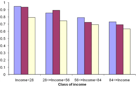
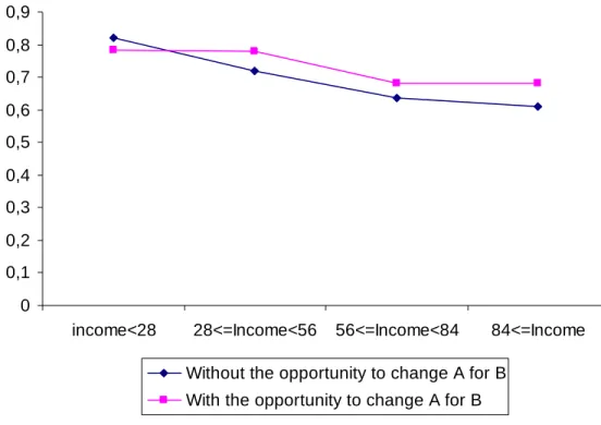
(16) Apart from the differences in the overall reporting rate across the treatments discussed above, we also observe that the participants not reporting any income are more numerous in the monitoring treatment with the opportunity of transfers compared to the monitoring treatment without the opportunity of transfers. The percentage of participants reporting no positive income goes from 0.05% in the treatment without transfers to 1.54% when it is possible to avoid units of A by purchasing units of B. Figures 1a and 1b provide additional information about the effects of monitoring and announcement respectively for sessions 1-8 (monitoring treatment without opportunity of transfer was in effect) and sessions 9-16 (monitoring treatment with opportunity of transfer) by each level of income. [Figures 1a and 1b about here] Both figure 1a and 1b show that the reporting level in the baseline treatments is greater than 70% for every income range. Positive and relatively high reporting rates indicate that the majority of the participants are either risk averse or that other suggested models of tax compliance are at play here.11 We also observe that in all treatments, reporting rate decreases with the level of income. Turning next to the differences between treatment, Figure 1a shows that announcement induces a significant reduction of overall reporting rate. In contrast, perfect monitoring seems to have two opposite effects depending on the level of income. The effect of an increase in monitoring seems to have a negative effect on reporting rate for lower incomes whereas it has a positive effect on this ratio for higher incomes. Considering now Figure 1b, we observe that perfect monitoring induce a reduction in the reporting rate level. Consistent with our previous results, the negative effect of announcement is lower in this case compared to figure 1a, which indicate that subjects are aware that the introduction of perfect monitoring is less dramatic when they have the opportunity to transfer income to the unmonitored source. Finally, the negative effect of perfect monitoring (significant at 5%) compared to 11. Recall that under the risk neutrality condition, it is very profitable for the participant to report nothing as their income.. 13.

(17) the baseline treatment indicates that increasing monitoring does not necessarily improve reporting rate when individuals have the opportunity to transfer income to unmonitored source. Table 2 presents descriptive statistics by participant income-type (80%, 50%, 20% of total income generated from source A). Table 2 shows that the participants who had 80% of their income generated from source A were obliged to report more income than they would have if not monitored so closely. [Table 2 and Figure 2 about here] Figure 2 also provides additional information, showing that the participants who had 80% of their income from source A tend to increase their reporting rate in the monitoring treatment (both with and without transfers) and in the announcement treatment compared to the baseline treatment (significant at 5%). In sharp contrast, the two other types of participants (e.g. with 50% and 20% of income from source A) significantly reduce their reporting rate.12 Figures 3, 4 and 5 compare the two monitoring treatments with an opportunity of transfers and without the by participant income-type. The two player types of interest are the participants that have the most monitored income, those with 80% and 50% of income from source A. The declaration rates are generally lower and especially lower for high income periods when participants had the opportunity to transfer income from Source A to Source B. For the least monitored participants, those with only 20% of total income derived from Source A, the difference between the two treatments is insignificant. The participants’ inclination to avoid being in the reported income’s lower bracket, and by the same token to face a 20% auditing rate, explains this result. Actually, since buying extra units of B is costly, it would be useless to do so if one had to report it. The participant knows that, having 80% of his total income already not systematically audited, part of this income will have to be reported to try to avoid the higher auditing rate.. 12. To a large extent, these results are comparable to those of Alm and McKee (2006) who found that ‘announcement increases compliance of those told they will be audited, but reduces compliance of those knowing they will not be audited; the net effect is that overall compliance falls’.. 14.

(18) [Figures 3, 4 and 5 about here] 4.2 Econometric Results The descriptive statistics imply that the perfect monitoring of matched income does not bring in greater tax revenues for the government.13 In fact, tax revenues will decrease with perfect monitoring with respect to the parameters of the experiment. Two primary factors can explain this result. First, as the descriptive statistics for the monitoring treatment without opportunity of transfers shows, participants tend to cheat more on unmonitored income when they cannot underreport monitored income. The only exception in this study is the subgroup of participants whose income from Source A represents 80% of their total income. Second, there is a shift towards unmonitored income (Source B) when this option is available for the highly monitored participants (80% and 50% from Source A). A reasonable explanation for these observations is that participants are willing to assume more risk when they are closely monitored in order to maintain a net expected income comparable to what they had before the introduction of monitored income. The results from the random effects QGLS regressions reported in Table 3 confirm the diminution of tax revenues. We consider two specifications. In specification (1), we only take into account the experimental parameters and behaviors recorded. In specification (2), we add various participantcharacteristics: age; sex; previous participation is a binary variable for whether the participant has already taken part in an experiment other than the current one (0 = no participation, 1 = participated in a previous experiment); gamble indicates whether the participant chose to earn a guaranteed $5 showup fee, or a gamble with a 50% probability of earning $11 and a 50% probability of earning $0. Participants who choose the gamble are considered less risk averse than the others; instruction feedback describes the participant’s assessment of the clarity of the instructions on a scale of 0 to 10, 10 being 13. Tax revenues are the tax paid on the reported income. They do not include penalties.. 15.

(19) “very clear”; and a list of binary variables indicating whether the participant is a worker, unemployed, a student, a graduate student and a student with prior mathematical training).14 [Table 3 about here] With respect to the reference treatment that is the basic treatment preceding the announcement and policy implementation treatments, we observe that the tax revenues decrease when we allow a shift towards cash payments in the perfect monitoring treatments. The tax revenues decrease by 1.044 eu, 3.2966 eu and 2.7286 eu with respect to the basic treatment for participants with respectively 80%, 50% and 20% of their initial income coming from source A.15 If the participants are not able to shift income from Source A to Source B, the tax revenues increase by 3.478 eu for those participants with 80% of their initial income coming from source A when comparing the basic treatment with perfect monitoring of matched income. Tax revenues are stable for participants with 50% of their income coming from A and it decreases by 1.6383 eu for those with 20% of their income coming from source A. In the announcement treatment preceding the introduction of the perfect monitoring without opportunity of transfers of matched income treatment, the tax revenues decrease with respect to the reference treatment. In the announcement treatment preceding the introduction of the perfect monitoring with opportunity of transfers, there is no diminution in tax revenues.16 We conjecture that the difference in behavior between the treatments is that the participants are trying to counteract the. 14. Given. RFit measuring the taxes paid (tax revenues) by participant i at period t. Tax revenues are described by a vector. of exogenous variables zit and the corresponding vector with parameters δ, and a random variable that can be divided into a random individual effect. α i , and a pure random variable ε it : RFit = zit δ + α i + ε it , i = 1,… , n, t = 1,… , T , with. the usual hypotheses on the different random variables. Using the results from Table 3, the calculations for the type II are: with respect to the reference state, we must add the coefficient 0.0439 of ″Type II (both treatments)” to the coefficient – 3.3404 of “Type II and transfer”. 16 The diminution is in fact smaller as shows by the positive coefficient, which is, however, relatively les significant then the others. 15. 16.

(20) eventual consequences of the perfect monitoring system by taking advantage of their current situation. The participants with the opportunity to transfer incomes seem to understand that they can avoid taxes even after perfect monitoring is implemented, whereas they cannot do this in the treatment without transfers. Consequently, they do not have the same motivation to “stock up” before the new policy with transfers is implemented. We have seen earlier that the reporting rates decrease with the income. Nonetheless, table 3 shows that tax revenues increase with the income since the income raise compensates for the diminution of the reported income. Finally, we observe that the participants reduce their reported income in the period following an audited period. This results in smaller tax revenues. Again, the idea here is to compensate for the losses suffered in the audit (this is known as a reference-dependence effect, Tversky and Kahneman 1991). This occurrence could also be explained by the “gambler fallacy” concept, which states that the participants believe that after being audited once, the probability to be audited two times in a row is smaller. This is of course incorrect, the auditing probabilities being independent from a period to the next. The second econometric specification controls the previous results with the addition of variables on the participants’ characteristics. It is interesting to notice that they do not affect the experimental variables’ estimated coefficients. Nonetheless, some characteristics of the participants play a role in the decisions or strategies used. A male participant reports a lesser income than a female participant (everything else being equivalent). In numerous studies, it is suggested that men are less risk averse than women. As it seems to be slightly the case in our experiment, we can expect participants who have already taken part in an experiment (we make sure that no participant takes part in the same experiment or a similar one twice) to learn faster to find the most lucrative strategy. We do not have a specific explanation for the. 17.

(21) positive estimated coefficient of the age and feedback variables, nor for the negative coefficient of the workers.. 5. Conclusion The motivation for this study was to examine the impact of perfect monitoring of matched income on tax compliance. To address this question, we used a laboratory experiment to observe actual and reported income behavior in a repeated decision framework. Two treatments were used to observe the change in monitoring with and without the opportunity to transfer income from the perfectly monitored source to the unmonitored source. We have three key findings. First, on average the less monitored income types (50% and 20% from Source A) and all income types when allowed to transfer income had higher rates of non-compliance. The only group that had the same rate of compliance was the group that derived 80% of their income from Source A without the opportunity to transfer incomes. Second, when the participants have the opportunity to get rid of their automatically audited income, they more than compensate for the mandatory taxes on Source A income and pay less overall on Source B income. Third, we find a significant decrease in tax revenues with the opportunity of transfers. We observe a drop of approximately 15% of the tax revenues with the realistic treatment with transfers of incomes. We do not pretend that a 15% tax reduction will be seen, but we are convinced that, if perfect monitoring is instituted without other complementary policies, an increase in tax revenues is not the likely outcome. This study stresses the point that a successful policy aiming at reducing fiscal fraud might be a difficult task, once people have decided their equilibrium level of tax compliance. The reference-dependent effect observed in the data suggests that individuals will try to recover their losses following any policy. 18.

(22) changes even if it means taking more risks.17 May be the only solution is to assess what taxpayers consider a ¨fair¨ level of taxation, which balance their relative level of tax contributions with what they expect to gain from them.. 17. It is interesting to note that this risk attitude is found in conductors driving their car. Additional security improvements to the car appear to induce drivers to keep constant their level of risk by taking more chances on the road. This is referred to the hysteresis assumption.. 19.

(23) References Allingham, M.G. and A. Sandmo, “Income Tax Evasion: A Theoretical Analysis.” Journal of Public Economics 1 (November). 1972: 323-338. Alm. J., B.R. Jackson and M. McKee “Estimating the Determinants of Taxpayer Compliance with Experimental Data.” National Tax Journal 45 (March). 1992: 107-114. Alm, J., C. Blackwell and M. McKee, Äudit Selection and Firm Compliance with a Broad-based Sales Tax.¨ National Tax Journal 57 (June). 2004: 209-227. Alm J. and M. McKee, Äudit Certainty, Audit Productivity and Taxpayer Compliance.¨ National Tax Journal 59 (December). 2006:801-16 Andreoni. J., B.Erard and J. Feinstein, “Tax Compliance.” Journal of Economic Literature 36 (June). 1998: 818-860. Blumental. M., C. Christian and J. Slemrod. “The Determinants of Income Tax Compliance: Evidence From a Controlled Experiment in Minnesota.” National Bureau of Economic Research Working Paper No. 6575. 1998. Boylan, S. and G. Sprinkle. Ëxperimental Evidence on the Relation between Tax Rates and Compliance: The Effect of Earned vs. Endowed Income. Journal of the American Taxation Association, 23 (1). 2001: 75-90. Cadsby C.B., E. Maynes, and V.U. Trivedi, ‘Tax compliance and obedience to authority at home and in the lab: A new experimental approach’ Experimental Economics, 2006, 9:343-359. Clotfelter, C. ¨Tax Evasion and Tax Rates: An Analysis of Individual Returns.¨ Review of Economics and Statistics, 65 (3). 1983: 363-373. Dubin. J. A., M.J. Graetz and L.L. Wilde. “The Effect of Audit Rates on the Federal Individual Income Tax. 1977-1986.” National Tax Journal 43(4). 1990: 395-409. Erard, B. and C. Ho (2001). ¨Searching for Ghosts: Who Are the Nonfilers and How Much Tax Do They Owe?¨ Journal of Public Economics 81. 2001 : 25-50. Fortin B., G. Garneau, G. Lacroix, T. Lemieux, and C. Montmarquette. “L'économie souterraine au Québec” Mythes et réalités, Sainte-Foy: Presses de l’Université Laval. 1996. Gërxhani, K and A. Schram (2006). ¨Tax evasion and income source: A comparative experimental study¨. Journal of Economic Psychology, 27( 3). 2006: 402-422. Internal Revenue Service. Federal Tax Compliance Research: Individual Income Tax Gap Estimates for 1985. 1988. and 1992. IRS Publication 1415 (Rev. 4-96). Washington. D.C. 1996. Jackson B.R. and V.C. Milliron. ¨Tax compliance research: Findings, problems and prospects¨. Journal of Accounting Literature 5. 1986: 125–165.. 20.

(24) Kahneman. D. and A. Tversky (1979). "Prospect Theory: An Analysis of Decision under Risk". Econometrica 47. 263-91. Mikkensen J.L. Äudits and the tax base: Evidence on Induced sales tax noncompliance¨. Western Tax Review 6. 1985: 86-114. Murray M.N. "Sales Tax Auditing and Compliance". National Tax Journal, 48. 1995: 515-530. Lippert O. And M. Walker. Editors. The Underground Economy : Global Evidence of Its Size and Impact. Fraser Institute. 1997. Roth J.A. and J.T Scholz, Editors, Taxpayer Compliance, Volume 2, Social Science Perspectives. University of Pennsylvania Press: Philadelphia. 1989. Slemrod, J. Why People Pay Taxes: Tax Compliance and Enforcement. University of Michigan Press: Ann Arbor MI. 1992. Webley P., H. Robben, H. Effers and D. Hessing. Tax Evasion: An Experimental Approach. CambridgeUniversity Press: Cambridge. 1991.. 21.

(25) Table 1. Descriptive Statistics Basic treatment (both sessions 1-8 and 9-16). VARIABLES Average. Announcement treatment preceding monitoring without transfers (sessions 1-8). Announcement Perfect Monitoring treatment preceding monitoring with transfers treatment without transfers (sessions 1-8) (sessions 9-16). Perfect Monitoring treatment with transfers (sessions 9-16). Std Dev.. Average. Std Dev.. Average. Std Dev.. Average. Std Dev.. Average. Std Dev.. Total income — (in eu). 60,99. 28,72. 52,56. 28,00. 62,50. 30,34. 58,02. 27,17. 59,33. 28,52. Reported income — (in eu). 46,07. 30,65. 35,25. 27,86. 46,10. 29,65. 44,41. 26,98. 40,34. 27,50. Overall reporting rate — (in %). 79,04. 42,31. 69,87. 42,24. 78,73. 35,08. 78,59. 30,64. 70,94. 34,29. Reporting rate on B * — (in %). 67,78. 60,51. 55,24. 56,29. 63,06. 53,54. 56,88. 51,44. 55,85. 44,55. Taxes paid on the reported income. 18,16. 12,25. 13,83. 11,09. 18,15. 11,84. 17,45. 10,81. 15,83. 11,02. 6,20. 11,08. 25,16. 36,23. Amount of B purchased — (in eu) Amount of B purchased over available — (in eu). B. —. —. —. —. —. —. —. —. % reporting no income. 5,46. 9,72. 4,86. 0,05. 1,54. % reporting their total income. 47,05. 38,72. 42,36. 39,48. 38,05. % reporting no income on B. 26,17. % Auditing. 14,21. * For the basic and announcement treatment:. 31,42 —. 13,37. 25,17 —. 13,37. 24,80 —. 13,89. 23,07 —. 15,97. —. (reported income – income from A) /(income from B). 22.

(26) Table 2. Descriptive Statistics. Monitoring treatment without opportunity of transfers Sessions (1-8) VARIABLES. Type I 80% of income from Source A Average. Std Dev.. Type II Type III 50% of income from 20% of income from Source A Source A Average. Std Dev. 27,18. Monitoring treatment with opportunity of transfers Sessions (9-16) Type I 80% of income from Source A. Std Dev.. Average. Std Dev.. Average. Std Dev.. Average. Std Dev.. 58,02. 27,18. 59,33. 28,53. 59,33. 28,53. 59,33. 28,53. 43,53. 26,17. 35,63. 26,27. 41,87. 29,36. 36,63. 72,82. 36,41. 58,02. 27,18. 58,02. Reported income — (in eu). 52,11. 24,51. 43,70. 24,00. 37,41. 30,00. Overall reporting rate — (in %). 90,63. 10,63. 77,06. 27,55. 68,09. 41,09. 75,56. Reporting rate on B * — (in %). 55,42. 49,32. 54,70. 54,07. 60,54. 50,70. 45,08. Taxes paid on the reported income. 20,51. 9,80. 17,15. 9,63. 14,68. 12,03. Amount of B purchased — (in eu) —. % reporting no income. 0,00. % reporting their total income. 42,41. % reporting no income on B. 26,79. % Auditing. 14,29. —. —. —. 0,00. —. Type III 20% of income from Source A. Average. Total income — (in eu). Amount of B purchased over B available — (in eu). Type II 50% of income from Source A. —. —. 28,21. 64,43. 45,49. 52,87. 44,41. 69,59. 17,08. 10,46. 13,96. 10,54. 16,45. 11,78. 7,74. 14,32. 7,93. 11,25. 2,94. 4,63. 17,99. 30,11. 30,00. 38,21. 27,50. 38,66. 0,15. 0,89. 1,93. 1,79. 41,82. 34,23. 37,50. 34,08. 42,56. 27,53. 17,11. 36,01. 17,86. 15,33. 12,80. —. 14,58. —. 14,88. —. 18,60. —. 14,43. 40,03. —. 23.

(27) Table 3. Tax Revenue Determinants Tax Revenues Panel data QGLS regressions (9024 obs) Total income. Model (1). Model (2). 0.2506*** (0.0026) -1.0377*** (0.2113) Ref. -1.6418*** (0.3280) 0.7809* (0.4611) 3.4780*** (0.3624) -4.5220*** (0.5106) 0.0439 (0.3625) -3.3405*** (0.5109) -1.6383*** (0.3624) -1.0986** (0.5106). 0.2506*** (0.0026) Previous period audit or non-audit -1.0408*** (0.2113) Basic Ref. Announcement (both treatments) -1.6531*** (0.3280) Announcement and transfer 0.8033* (0.4613) Type I (both with and without transfers) 3.4478*** (0.3619) Type I and transfer -4.4590*** (0.5105) Type II (both with and without transfers) 0.0059 (0.3620) Type II and transfer -3.3061*** (0.5099) Type III (both with and without transfers) -1.6034*** (0.3622) Type III and transfer -1.1296** (0.5105) Age 0.1796*** (0.0672) Men -3.6420*** (0.7077) Previous participation -1.5496** (0.7471) Gamble 0.0897 (0.7868) Instruction Feedback 0.4916** (0.2394) Worker -3.5577*** (1.3432) Unemployed 0.0217 (1.4523) Student Ref. Ref. Graduate student -0.7124 (0.9061) Mathematical training -0.8269 (0.7393) Constant 2.9535*** -2.1926 (0.4122) (2.5930) ρ 0.3441** 0.303** The first period of observation was eliminated due to the construction of the lagged audit variable.. The correlation coefficients ρ are statistically significantly different from ″0″ according to the Lagrange multiplier test with a 5% critical threshold. Standard errors in parentheses: * significant at 10%; ** significant at 5%; *** significant at 1%.. 24.

(28) Figure 1a. Ratio of reported income per class of income (session 1-8). Figure 1b. Ratio of reported income per class of income (session 9-16). 25.

(29) Figure 2. Ratio of the reported income per type. 26.

(30) Figure 3. Ratio of the reported income for those having 80% of their income automatically audited (source A). 1 0,9 0,8 0,7 0,6 0,5 0,4 0,3 0,2 0,1 0 income<28. 28<=Income<56 56<=Income<84. 84<=Income. Without the opportunity to change A for B With the opportunity to change A for B. Figure 4. Ratio of the reported income for those having 50% of their income automatically audited (source A). 0,9 0,8 0,7 0,6 0,5 0,4 0,3 0,2 0,1 0 income<28. 28<=Income<56 56<=Income<84. 84<=Income. Without the opportunity to change A for B With the opportunity to change A for B. 27.

(31) Figure 5. Ratio of the reported income for those having 20% of their income automatically audited (source (A)). 0,9 0,8 0,7 0,6 0,5 0,4 0,3 0,2 0,1 0 income<28. 28<=Income<56. 56<=Income<84. 84<=Income. Without the opportunity to change A for B With the opportunity to change A for B. 28.

(32) Appendix: Participant instructions (translated from French) General Instructions. You are asked to participate in a series of decisions. This experiment is made of several periods. You will be asked to make a decision in each period. You must complete one period before moving on to the next period. Your earnings depend on what you decide. Therefore, it is important to read these instructions carefully. At the end of the experimental session, you will make a random draw from all the played periods. Your earnings for the session will be a function of your “net final income” from that period. What you earn is completely private. You will be paid for one randomly selected decision (period) in private at the end of the experiment.. Period Breakdown.. Every period, you will receive your income. This income is randomly drawn by the computer and is between 10 eu (experimental units) and 110 eu. Two sources of income. Your income comes from two different sources: A and B. There are three participant types randomly determined by the computer. They are characterized by whether most of their income comes from source A, source B, or equally from both sources. That is ¾ ¾ ¾. Type 1: Type 2: Type 3:. 80 % of your total income comes from source A and 20 %, from source B. your total income comes equally from sources A and B. 20 % of your total income comes from source A and 80 %, from source B.. For example, suppose that you are a type 3 player. If your total income is 50 eu, 10 eu would come from source A and 40 eu would come from source B. This information is confidential. You remain of the same type for the entire experiment. Paying taxes. Only you know your true income. Once you know your true income, you will be asked to report your income to the government and pay taxes on the reported income. There is no restriction on how much you can report (apart from it being a non-negative whole number – no decimals). You can report more, the same or less than your true income. Your earnings at the end of the experiment depend on your true income less taxes paid and possible fines. Once you have reported your income, a 40% tax is levied on this reported income.. 29.

(33) Auditing. The government does not know your true earned income nor whether your income from source A is 80%, 50% or 20% of total income. Only you know this. The government could audit you and everyone else in the room and discover your income, but this is very expensive and useless if you already reported your true income. Therefore, the government randomly audits people and the probability to be audited is a function of the following rule: • If your reported income is in the bottom 50% of the reported incomes, the probability to be audited is 20%. • If your reported income is in the top 50% of the reported incomes, the probability to be audited is 10%. If you are audited and it reveals that you have under-reported your total income, you will have to pay: 1) the taxes on the non-reported income, and 2) a fine corresponding to 50% of the overdue taxes that you had not reported. In other words, you would be paying one and half times the unpaid taxes. Additionally, if audited, you will automatically be audited for the previous 2 periods. If you had underreported your income in these periods, you will have to pay 1.5 times the unpaid taxes for each one of these periods as well. Hence. your “net final income” for the audited period is equal to your reported income less the taxes paid on your reported income less the sum of the overdue taxes and fines for the current period (t) and the previous 2 (t-1 and t-2), if applicable. Note that you can not be audited (and fined) twice for the same period. How your earnings from the experiment are determined. Every period, your “net final income” is determined by the computer the following way: •. If you are not audited:. ”Final net income” = Total income – Taxes on the reported income •. If you are audited and have reported your total income:. ”Final net income” = Total income – Taxes on the reported income •. If you are audited and have not reported your final income:. ”Final net income” = Total income – Taxes on the reported income – Taxes on the non-reported income (in t. t-1 and t-2) – Fines (in t. t-1 and t-2). As a reminder, taxes on the reported income are 40% of the reported income, the taxes on the nonreported income (payable if audited) correspond to: 40% X (total income – reported income). Finally,. 30.

(34) the fine corresponds to 50% of the taxes on the non-reported income. (note that our program rounds up the decimals). At the end of the experimental session, you will randomly draw a number corresponding to one of the played periods. Each number has an equal probability to be drawn. Your earnings in eu for the drawn period will be converted with a $1 eu = 0.50 $CAN rate. Additional information. We recommend you to re-read these instructions. After taking place in front of your computer, please raise your hand if you have questions regarding the instructions. We will come and answer them privately, and will then inform everybody in the room of both the question and the answer. The questions should not try to validate a decision strategy, but only attempt to understand the instructions better. Before we start the experimental session, we will ask you some questions regarding your age, gender, level of education and field of study, universities or schools currently attended, or your situation on the work market, and whether you have already participated in such an experiment. This information will remain anonymous. We will then begin the experiment. We will also so ask you some comprehension questions on these instructions.. 1st Announcement. Treatment I (given prior to period 22) We are only advising you that starting 6 periods from now, a new technology will allow the government to automatically know all the income you will earn from source A. However, as a reminder, the government will not know your total income nor which type of player you are (i.e. whether your income from source A is 80%. 50% or 20% of your income).. Following the introduction of this technology, since the government will know all the income coming from source A, you will be audited automatically if you report income less than what you receive from source A. We remind you that, as in the previous periods, when you are audited for a given period, you will be retroactively audited for the two previous periods as well. In other words, if you are audited in this upcoming period, you will automatically be audited for the last two periods before this new technology was announced.. 2nd Announcement. Treatment I (given prior to period 28) As promised, the new technology that allows the government to automatically know all the income you will earn from source A is in service.. 31.

(35) From now on, if you report income lower than received from source A, you will be automatically audited. The other conditions regarding the taxes, fines and audit are still in effect.. 1st Announcement. Treatment II (given prior to period 22) We are only advising you that starting 6 periods from now. a new technology will allow the government to automatically know all the income you will earn from source A. However, as a reminder, the government will not know your total income nor which type of player you are (i.e. whether your income from source A is 80%. 50% or 20% of your income). Furthermore, you will be able to purchase experimental units of source B with units of source A, at the specified rate.. Following the introduction of this technology, since the government will know all the income coming from source A, you will be audited automatically if you report income less than what you receive from source A. We remind you that, as in the previous periods, when you are audited for a given period, you will be retroactively audited for the two previous periods as well. In other words, if you are audited in this upcoming period, you will automatically be audited for the last two periods before this new technology was announced.. 2nd Announcement. Treatment II (given prior to period 28) As promised, the new technology that allows the government to automatically know all the income you will earn from source A is in service, you are able to purchase units of source B with units of source A. You must expend 1.25 units of A to obtain 1 unit of B. We specify that this technology allows the government to know your final number of units from A, but it does not know how much you initially had. Without auditing you, the government does not know your income from source B. If you decide to do such transactions, your gross income will be modified, but your taxable income will remain your initial given income. From now on, if you report income lower than received from source A, you will be automatically audited. The other conditions regarding the taxes, fines and audit are still in effect. If you have not purchased units of B with units of A, your “final net income” is calculated by the computer the same way as before. If you have purchased units of B with units of A. your “final net income” is calculated by the computer the following way:. 32.

(36) •. If you are not audited :. “Final net income” = Total income – Cost to purchase units of B– Taxes on the reported income. •. If you are audited and have reported your total income:. “Final net income” = Total income – Cost to purchase units of B – Taxes on the reported income. •. If you are audited and have not reported your total income:. “Final net income” = Total income – Cost to purchase units of B – Taxes on the reported income – Taxes on the non-reported (initial) total income (in t. t-1 and t-2) – Fines (in t. t-1 and t-2). 33.

(37)