HAL Id: hal-02089227
https://hal-univ-rennes1.archives-ouvertes.fr/hal-02089227
Submitted on 6 Jun 2019
HAL is a multi-disciplinary open access archive for the deposit and dissemination of sci-entific research documents, whether they are pub-lished or not. The documents may come from teaching and research institutions in France or abroad, or from public or private research centers.
L’archive ouverte pluridisciplinaire HAL, est destinée au dépôt et à la diffusion de documents scientifiques de niveau recherche, publiés ou non, émanant des établissements d’enseignement et de recherche français ou étrangers, des laboratoires publics ou privés.
tunnel experiments
M.C.S. Ferreira, B. Furieri, Ahmed Ould El Moctar, J.-L. Harion, Alexandre
Valance, P. Dupont, N.C. Reis, J.M. Santos
To cite this version:
M.C.S. Ferreira, B. Furieri, Ahmed Ould El Moctar, J.-L. Harion, Alexandre Valance, et al.. A simple model to estimate emission of wind-blown particles from a granular bed in comparison to wind tunnel experiments. Geomorphology, Elsevier, 2019, 335, pp.1-13. �10.1016/j.geomorph.2019.03.004�. �hal-02089227�
ACCEPTED MANUSCRIPT
Geomorphology
A simple model to estimate emission of
wind-blown particles from a granular bed in
comparison to wind tunnel experiments
M. C. S. Ferreira, B. Furieri, A. Ould El Moctar, J.-L. Harion, A.
Valance, P. Dupont, N. C. Reis Jr, J. M. Santos
Department of Environmental Engineering, Universidade Federal do Espírito Santo, 29075-910, Vitória, ES, Brazil
Department of Mathematics, Instituto Federal do Espírito Santo, 29040-780, Vitória, ES, Brazil
Laboratoire de Thermique et Energie de Nantes, UMR CNRS 6607, 44306 Nantes, France IMT Lille-Douai, 59500 Douai, France
Institut de Physique de Rennes, CNRS UMR 6251, Université de Rennes, 35042 Rennes Cedex, France
LGCGM, EA3913, Université de Rennes, 35042 Rennes Cedex, France
Abstract
Dust emissions due to aeolian erosion of exposed granular materials are strongly influenced by grain size distribution. Non-erodible particles that are too heavy to be lifted into the air play a protective role in the aeolian erosion process attenuatingemission, which is known as the pavement phenomenon. To date, there is no approach that reliably predicts the reduction in emissions caused by their presence on an aggregate surface. In this work, an analytical model was developed to quantify emissions from particle beds with a wide size distribution. As non-erodible particles accumulate, changes in surface characteristics create increasing shelter for the erodible portion of the bed until the shear on the erodible surface reaches a minimum and emissions cease. The proposed emission model describes the relationship between this minimum value of wind shear and the eroded depth of the bed after the pavement, which in turn gives the emitted mass. In addition, wind tunnel experiments were carried out in order to broaden knowledge of the pavement phenomenon and validate the modelling. A bimodal particle size distribution of sand with erodible and non-erodible particles was used for the tested velocities. Three experimental measurements were carried out: (i) continuous weighing of the emitted mass, (ii) eroded depth of the bed at regular time intervals and (iii) final cover rates of the non-erodible particles using digital analysis of sand bed pictures after experiments. Good agreement between the modelling and experimental results was found. The emission model proposed herein is a simple algebraic expression that demands low computational effort. This approach may serve as a base for an emission model for application in granular materials stockpiles.
Keywords: Wind Erosion, Non-erodible Particles, Fugitive emissions, Emission model
1. Introduction
Wind erosion is a natural process characterised by particle entrainment, transport and deposition due to the action of wind. The understanding of the phenomenon is important in several research fields such as land degradation in agricultural areas [58,2], deserts expansion [20], dunes morphology and dynamics [6,9], dust storms [29], design of porous
ACCEPTED MANUSCRIPT
fences to prevent soil erosion [31] and air pollution [5]. Particulate air pollutants have diverse chemical compositions and cover a wide range of sizes, from 0.001 nm to 100 𝜇𝑚. Although the particles larger than 10 𝜇𝑚 have a shorter atmospheric lifetime and settle closer to the sources of emission, they can cause annoyance related to dirtiness, eye irritation, cough and allergic reaction. The long-range transport of the smallest particles, such as 𝑃𝑀10 (< 10 𝜇𝑚), 𝑃𝑀2.5 (< 2.5 𝜇𝑚) and ultrafine particle fractions (< 0.1 𝜇𝑚), can reach atmospheric lifetimes of days, weeks, or even years [46]. These particles are responsible for a variety of serious harmful effects on health, especially related to cardiovascular and respiratory diseases [55].
Emissions due to aeolian erosion of exposed granular materials are strongly influenced by the grain size distribution possibly presenting coarse particles that are not lifted by wind flow [17,48,49,57]. In the range of investigated wind velocities, the basal shear stress is insufficient to lift the large particles of 1 mm in diameter, referred hereafter as non-erodible particles. Wind erosion processes and emission estimation have been studied by numerical and experimental approaches. Several experimental studies have shown that the presence of these non-erodible particles affects dust emission limiting the availability of particles supply and promoting a temporal decrease in emitted mass flux [33,30,32,11,53,25]. As the surface is eroded, the coarse particles accumulate and protect the bed surface from erosion, which is known as the pavement phenomenon. Therefore, it is important to consider temporal variability in surface conditions to develop wind erosion models [41,54,37]. Nonetheless, aeolian transport is often viewed as a steady-state process, and most available emission models are applied to particle beds with a homogeneous size distribution. Some models account for the wide range of particle sizes in the bed [35,1,28], however, modifications of soil size distribution with time are not usually considered. The work of [12] was the first attempt to fill this gap. The authors developed a stochastic model that quantifies the temporal evolution of the emitted mass flux in a bed of granular material with a wide size distribution exposed to a turbulent flow. To model pavement, [12] assumed that erosion is finalised when the bed is completely overlaid by non-erodible particles. However, experimental results showed that when erosion stops, potential erodible particles still remain on the surface [11,17]. The accurate prediction of the phenomenon is a complex task due to the uncertainty in the transport processes. [42] describe in their paper this inherent uncertainty in the saltation phenomenon. [36] presented a new methodology for characterizing high-frequency fluctuations of aeolian saltation flux.
The present work aims to investigate the pavement phenomenon and propose an emission model, which includes a new approach to characterise the influence of non-erodible particles accumulation. The non-erodible particles protect the erodible surface by both covering the surface and creating downstream wake zones of reduced wind shear stress on the intervening bare surface [19,23,44,38,40]. As the concentration of larger particles in the bed increases, the mean shear on erodible surfaces decreases until it is no longer significant to cause emissions. Thus, pavement modelling in the proposed model is related to the wall shear stress evolution as wind erosion modifies the surface. The partition of shear between non-erodible particles and adjacent erodible ones is investigated using numerical simulations of turbulent flow over a rough surface and a mathematical formulation to associate the geometrical characteristics of the non-erodible particles and the mean friction velocity on the erodible surface (Section 2). Based on this formulation, the final conditions of the bed, such as the eroded depth and the cover rate of non-erodible particles, were determined byassuming that after pavement, the friction velocity reaches a minimum value. Then, besides providing the emitted mass from a particle bed, the model gives the final state of the bed topography (Section 3). The primary objective of this study is to propose a simple model for dust and particle emission in practical situations such as in industrial sites of storage piles of granular material or in semi-arid
ACCEPTED MANUSCRIPT
environments (soil erosion) from the knowledge of the distribution of the surface friction at the local level. An experimental study in a wind tunnel, described in Section 3, was conducted to validate the modelling results (final characteristics of the bed surface and global emissions estimates).
The primary objective of this study is to propose accurate and simple models for dust and particle emission in practical situations such as in industrial sites of storage piles of granular material or in semi-arid environments (soil erosion). The main ingredient of the model is the knowledge of the distribution of the surface friction at the local level. The only requirement to apply this model at regional scale for dust emission prediction is to assess the surface shear distribution linked to the local roughness. The purpose of the wind tunnel study is to validate this model in well-controlled situations.
2. Erosion model
1. Grain entrainment and saltation
Wind erosion of a particle bed is initiated by aerodynamic entrainment, whenever the velocity exceeds a critical value called the static threshold. The onset of grain motion is commonly described by the Shields number Θ, defined as the ratio between the shear force exerted by a fluid on a particle at the bed surface and the effective particle weight:
Θ = 𝜌𝑢
∗2
(𝜌𝑃− 𝜌)𝑔𝐷 ,
(1)
where 𝑢∗ is the friction velocity, 𝜌 is the fluid density, 𝜌𝑃 is the particle density, g is gravity and D is the particle diameter.
[3] investigated the static threshold Shields number Θ𝑆 (corresponding to the static threshold
friction velocity 𝑢𝑡∗𝑠) based on the balance of forces acting on a particle. The author found that Θ𝑆 is nearly constant for large particles (Θ𝑆 ≈ 0.01), which implies that 𝑢𝑡∗𝑠 increases with
√𝐷 in these cases. However, for small particles, Θ𝑆 is not constant and increases rapidly as
diameter decreases. As particle sizedecreases, inter-particle cohesion forces can no longer be neglected and its effect plays a dominant role in controlling threshold motion conditions. Since the pioneering work of [3], other studies have been devoted to investigating the threshold Shields number and erodibility conditions for the particles [24,15,8,14,13]. In the present work, the erodibility of the particles was assessed by a take-off criterion obtained by [47], who presented a simple expression relating the threshold friction velocity 𝑢𝑡∗𝑠 and the particle diameter D:
𝑢𝑡∗𝑠 = 0.11√𝜌𝑃− 𝜌
𝜌 𝑔𝐷 +
𝛾
𝜌𝐷 , (2)
where 𝛾 is a surface energy that characterises the cohesion.
Equation 2 implies that if inter-particle cohesion is considered, 𝑢𝑡∗𝑠 is proportional to √𝑐1𝐷 + 𝑐2𝐷−1 (instead of √𝐷). For large particles, the term 𝑐
1𝐷 dominates over 𝑐2𝐷−1,
which is consistent with Θ𝑆 ≈ 0.01. This criterion is in good agreement with a large number of
wind tunnel measurements [27]. [47] recommended values of 𝛾 ranging between 1.65 × 10⁻⁴ and 5.00 × 10⁻⁴ 𝑘𝑔/𝑠2. In this work, 𝛾 = 2.86 × 10⁻⁴ 𝑘𝑔/𝑠2 was used, as obtained
by [26] experimentally fitting Equation 2 to the threshold required to lift erodible particles. The take-off criteria (illustrated in Fig. 1) allows the estimation of the range of particle sizes
ACCEPTED MANUSCRIPT
liable to take-off by aerodynamic entrainment. For a given friction velocity 𝑢∗, there will be a range of critical diameters in which particles are emitted. Outside of this range, particles remain on the surface due to gravitational forces for larger particles and high cohesion forces for smaller particles.
Figure 1. Criteria for the definition of particles erodibility obtained by [47]
In the early stage of erosion, aerodynamic forces are mainly responsible for the entrainment of particles. Transport is initiated by aerodynamic entrainment of a small number of particles if the static threshold Θ𝑆 is reached. These particles may hop along the surface, and the impact of saltating grains on the bed surface can eject other particles. After saltation has initiated, subsequent lifting of surface particles occurs predominantly due to impact. Then, transport can be sustained even below the static threshold. The minimum velocity at which the combined action of wind forces and saltation impacts are capable of retaining particles in movement is called the dynamic threshold (Θ𝐷). The dynamic threshold is lower than the static threshold and is also fairly constant (Θ𝐷 ≈ 0.008 ) for large grains [7,22,8,14]. For smaller particles (typically ≲ 100𝜇𝑚), there is an increase in Θ𝐷 due to the importance of cohesion forces.
The expression of the threshold friction velocity versus the particle diameter presented herein (Equation 2) was developed for beds composed of particles with monodispersed size distribution, without roughness elements as non-erodible particles. The effects of the presence of roughness elements are taken into account by the shear stress distribution between the roughness elements and the ground surface.
2. Shear stress partition
The shear stress partition has been investigated by several researchers by means of theoretical [43,35] and experimental [34,10] approaches. Despite the importance of these works, they present shortcomings, most of all concerning large variations found in model parameters and the limited range validity for certain types of rough surfaces. Computational Fluid Dynamics (CFD) is a valuable alternative that can be applied to simulate the flow over surfaces with different shapes and arrangements of roughness elements. Different configurations may be too costly and time consuming to be predicted by experimental techniques.
[45] proposed that the total drag 𝜏 imparted to a rough surface can be written as: 𝜏 = 𝜌𝑢∗2 = 𝜏
𝑅 + 𝜏𝑆 , (3)
where 𝜏𝑅 is the pressure drag on the roughness elements and 𝜏𝑆 is the friction drag on the ground surface.
The shear stress 𝜏𝑆′ acting on the exposed surface (erodible), which drives wind erosion, is related to 𝜏𝑆 by:
𝜏𝑆′ = 𝜌𝑢 𝑆∗2=
𝜏𝑆
1 − 𝐶𝑅 , (4)
where 𝑢𝑆∗ is the mean friction velocity on the erodible fraction of a rough surface and 𝐶𝑅 is the cover rate of the surface by the roughness elements.
A theoretical model was proposed by [43], based on the idea that the wake and drag properties of an isolated roughness element can be characterised by an effective shelter area and volume. The shelter area describe the surface stress deficit behind the element and the shelter volume, the attenuation of drag on other obstacles in the element wake. It was assumed that the combined effective shelter can be calculated by randomly superimposing individual shelters. However, the validity of this hypotheses is limited to low values of roughness densities 𝜆. As
ACCEPTED MANUSCRIPT
𝜆 increases, element wake interactions become stronger and their collective effect cannot be described by superimposition. [43] model is given by:
𝜏𝑆′
𝜏 =
1
(1 − 𝜎𝜆)(1 + 𝛽′𝜆) , (5)
where 𝛽′ is the ratio of drag coefficient of an individual roughness element to the drag coefficient of the bare surface. The parameter 𝛽′ accounts for roughness element shape effects and entirely controls the partition of drag.
The [43] model has been assessed by several works in order to test and refine the parameters 𝛽′ [56,10,4,52]. A general conclusion is that the proposed formulation is valid, nonetheless,
presents shortcomings. [39] and [10] found that the parameter 𝛽′ has some degree of dependency on the aspect ratio of the roughness elements. The range of values obtained for 𝛽′ is relatively large, which makes difficult the identification of appropriate values for a specific surface with non-erodible elements [52].
[50] performed numerical simulations with different configurations of rough surfaces to depict the pavement process by determining the friction velocity experienced by the erodible fraction of particles as a function of the changes in bed topography, i.e., the increase in number or the height of the roughness elements. The work analysed the parameter 𝑅𝑓𝑟𝑖𝑐 (Equation 6), which reflects the evolution of the friction velocity applied to the exposed surface as erosion occurs:
𝑅𝑓𝑟𝑖𝑐 = 𝑢𝑆∗
𝑢0∗ , (6)
where 𝑢0∗ is the mean friction velocity on a surface without roughness elements. Then, [50] developed an empirical relationship to include the cover rate and particles geometrical parameters on 𝑅𝑓𝑟𝑖𝑐:
1 − 𝑅𝑓𝑟𝑖𝑐 = 𝐴(𝐶𝑅)𝑀(𝑆𝑓𝑟𝑜𝑛𝑡𝑎𝑙
𝑆𝑓𝑙𝑜𝑜𝑟 ) 𝑁
, (7)
where 𝑆𝑓𝑟𝑜𝑛𝑡𝑎𝑙 and 𝑆𝑓𝑙𝑜𝑜𝑟 are respectively the frontal and the basal areas of a cylindrical roughness element, and 𝐴, 𝑀 and N are coefficients determined by the numerical simulations. [16] found that Equation 7 is also valid for surfaces containing particles with different aspect ratios (non-uniform distribution of roughness elements). However, this formulation was tested for cover rates lower than 12%. Nonetheless, the particle size distribution found in nature, and particularly in granular materials from storage yards of industrial sites, can present higher cover rate values. Therefore, in the present study, additional numerical simulations were carried out in order to adjust the values of the coefficients 𝐴, 𝑀 and N for a larger range of cases. The studied configurations correspond to a bed of granular material, in which the non-erodible particles are represented by non-uniform cylindrical roughness elements randomly distributed, emerging at various levels from the surface (see Fig. 2). The transport of particles is not taken into account in the numerical simulations.
Figure 2. Random positioning of the non-uniform roughness elements in the numerical simulations
The parameters that define each test are: the range of roughness elements diameter 𝐷𝑟 and
height ℎ𝑟 (proportionally to 𝐷𝑟) and the number of roughness elements 𝑛𝑟 (𝑛𝑟 = 0
corresponds to a surface without roughness elements, i.e., 𝑢𝑆∗ = 𝑢0∗). The ratio 𝑆𝑓𝑟𝑜𝑛𝑡𝑎𝑙/𝑆𝑓𝑙𝑜𝑜𝑟 and the cover rate 𝐶𝑅 are determined for each simulated case according to:
𝑆𝑓𝑟𝑜𝑛𝑡𝑎𝑙 𝑆𝑓𝑙𝑜𝑜𝑟 = 4 𝜋 ℎ𝑟 𝐷𝑟 , (8)
ACCEPTED MANUSCRIPT
𝐶𝑅 = 𝜋
4 ∑ 𝐷𝑛𝑟𝑟 𝑟2
𝑆𝑏𝑒𝑑 , (9)
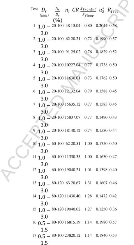
where 𝐷𝑟 and ℎ𝑟 are, respectively, the mean diameter and the mean emergent height of the roughness elements, and 𝑆𝑏𝑒𝑑 is the area of the bed. Table 1 presents the configurations of the simulated beds.
Table 1. Configurations of particle bed covered by cylindrical roughness elements tested in the numerical simulations. 𝒖𝑺∗ is the mean value of the friction velocity on the erodible surface, calculated using the
numerical results of the shear stress distribution. 𝑹𝒇𝒓𝒊𝒄 is calculated using Equation 6
Test 𝐷𝑟 (mm) ℎ𝑟 𝐷𝑟 (%) 𝑛𝑟 𝐶𝑅𝑆𝑓𝑟𝑜𝑛𝑡𝑎𝑙 𝑆𝑓𝑙𝑜𝑜𝑟 𝑢𝑆 ∗ 𝑅 𝑓𝑟𝑖𝑐 1 1.0 − 3.0 20-100 48 15.04 0.80 0.2044 0.58 2 1.0 − 3.0 20-100 62 20.21 0.72 0.1990 0.57 3 1.0 − 3.0 20-100 91 25.02 0.76 0.1829 0.52 4 1.0 − 3.0 20-100 102 27.04 0.77 0.1738 0.50 5 1.0 − 3.0 20-100 116 30.01 0.73 0.1762 0.50 6 1.0 − 3.0 20-100 121 32.04 0.79 0.1588 0.45 7 1.0 − 3.0 20-100 156 35.12 0.77 0.1583 0.45 8 1.0 − 3.0 20-100 158 37.07 0.77 0.1490 0.43 9 1.0 − 3.0 20-100 181 40.12 0.74 0.1530 0.44 10 1.0 − 3.0 60-100 62 20.51 1.00 0.1750 0.50 11 1.0 − 3.0 60-100 113 30.35 1.00 0.1630 0.47 12 1.0 − 3.0 60-100 190 40.21 1.01 0.1398 0.40 13 1.0 − 3.0 80-120 63 20.67 1.31 0.1607 0.46 14 1.0 − 3.0 80-120 114 30.40 1.28 0.1472 0.42 15 1.0 − 3.0 80-120 190 40.02 1.27 0.1250 0.36 16 0.5 − 1.5 80-100 168 15.19 1.14 0.1980 0.57 17 0.5 − 1.5 80-100 238 20.12 1.14 0.1840 0.53
ACCEPTED MANUSCRIPT
18 0.5 − 1.5 80-100 309 25.10 1.14 0.1721 0.49 19 0.5 − 1.5 80-100 410 30.19 1.14 0.1619 0.46 20 0.5 − 1.5 80-100 507 34.06 1.14 0.1510 0.43 21 0.5 − 1.5 140-160 168 15.11 1.90 0.1610 0.46 22 0.5 − 1.5 140-160 238 20.04 1.90 0.1601 0.46 23 0.5 − 1.5 140-160 309 25.03 1.90 0.1398 0.40 24 0.5 − 1.5 140-160 410 30.13 1.90 0.1332 0.38 25 0.5 − 1.5 140-160 507 34.12 1.91 0.1281 0.37The commercial software FLUENT was used to solve the three-dimensional Reynolds averaged equations of mass and momentum. The turbulence effects were accounted for by using the 𝑘 − 𝜔 Shear Stress Transport (SST) model. The turbulence model 𝑘 − 𝑒𝑔𝑎 SST is a RANS modelling presenting good accuracy and reduced computational effort required. It has been proven [51,18] that 𝑘 − 𝜔 SST model present better agreement with experimental and analytical data for the studied configuration, i.e., fluid flow surrounding obstacles than other RANS models such as 𝑘 − 𝜖, etc... The computation domain is represented by a parallelepiped (30 × 30 mm base and 100 mm height). Periodic conditions were applied to inlet and outlet boundaries, which means that the outlet was used to set the inlet profiles in a cyclic way until a fully developed flow was established. The simulations are initialized with a uniform velocity distribution, and the mass flow is fixed for a corresponding mean longitudinal velocity value equal to 8 𝑚/𝑠. The upper and lateral boundaries were defined as symmetry (normal gradients of all variables are set to zero) and the lower limits (roughness elements andground walls) as smooth walls with no-slip conditions.
The calculation domain was divided into two parts to allow a good mesh refinement near the wall in the spanwise and streamwise directions, with hexahedral and pentahedral elements, and a coarser mesh with quadrilateral elements elsewhere for better computational efficiency. This is necessary since strong velocity gradients and important fluid interactions occur near the wall. The height of the first mesh is 𝑧+ < 5 to ensure no use of wall functions in the turbulence model. Spanwise and streamwise mesh size in wall units (𝑥+ and 𝑦+) present a
maximum value of 10 which occurs far from the roughness elements. The smallest element size of the computational mesh is the cylinder circumference divided by about 20. The computationalset up (modelling choices including meshing, turbulence closure and domain configurations) was based on previously validated numerical calculations (cf. [50] and [16]). Fig. 3 shows the friction velocity contours on the erodible surface, determined from the shear stress distribution, for two different simulations: Tests 15 and 16. Test 15 presents higher values of the ratio 𝑆𝑓𝑟𝑜𝑛𝑡𝑎𝑙/𝑆𝑓𝑙𝑜𝑜𝑟 and 𝐶𝑅 than Test 16. Therefore, in Test 15, the wakes formed behind the elements are expanded and interact with the neighbouring particles, leading to a drop in the friction velocity on most of the underlying surface (see Fig. 3(a)) and a lower mean value of the friction velocity on the erodible surface (𝑢𝑆∗), as shown in Table 1.
Figure 3. Distribution of the parameter 𝑹𝒇𝒓𝒊𝒄 on the erodible surface for Tests (a) 15 and (b) 16
ACCEPTED MANUSCRIPT
𝐴 = 0.188, 𝑀 = 0.313 and 𝑁 = 0.216 through the least squares method. The relative errors between the numerical values of 𝑢𝑆∗ and those calculated by Equations 6 and 7 with the new coefficients do not exceed 5%. The proposed formulation was found to be in good agreement with the numerical results (𝑅2 = 0.97) (see Fig.4).
Figure 4. Correlation of 1-𝑹𝒇𝒓𝒊𝒄 results between numerical simulations and fitting of coefficients A, M and N
3. Roughness evolution and emission prediction
The main purpose of the erosion model is to determine particle mass emission based on the eroded depth of a particle bed for a given velocity, taking advantage of the formulation in Equation 7. The particles were assumed to be cylindrical, with height equal to the diameter of the base. The input variables of the model are wind velocity (𝑈∞), bed dimensions and the characteristics of the granular material. Given the particle size distribution, the mass fraction of particles 𝛼𝑖 for each size range of particles with representative diameter 𝐷𝑖 is:
𝛼𝑖 =
𝑀𝑖 𝑀𝑡𝑜𝑡 =
𝑉𝑖
𝑉𝑡𝑜𝑡 , (10)
where 𝑀𝑖 and 𝑉𝑖 are, respectively, the mass and the volume of particles from the range i, 𝑀𝑡𝑜𝑡 is the total mass of the particles and 𝑉𝑡𝑜𝑡 is the total volume occupied by the particles of the bed, calculated as:
𝑉𝑡𝑜𝑡= ∑ 𝑉𝑖
𝑖
= ∑ 𝑛𝑖
𝑖
𝑉𝐷𝑖 , (11)
where 𝑛𝑖 is the number of particles encompassed in the range of 𝐷𝑖 and 𝑉𝐷𝑖 is the volume of
one particle with diameter 𝐷𝑖 (for cylindrical particles 𝑉𝐷𝑖 = 𝜋𝐷𝑖3/4).
The total volume of particles is related to the volume of the (𝑉𝑏𝑒𝑑) through the volume fraction 𝜑:
𝜑 = 𝑉𝑡𝑜𝑡
𝑉𝑏𝑒𝑑 , (12)
which can be written as a sum of partial volume fractions 𝜑𝑖 of each diameter 𝐷𝑖:
𝜑 = ∑ 𝜑𝑖 𝑖 , (13) where: 𝜑𝑖 = 𝑉𝑖 𝑉𝑏𝑒𝑑 = 𝛼𝑖𝜑 . (14)
A spatial uniform distribution of particles was assumed along the height of the bed. For each representative diameter 𝐷𝑖 of a given size range, the number of layers in the bed height was calculated by dividing the height of the bed (𝐻𝑏𝑒𝑑) by 𝐷𝑖 (height of the particle). Therefore, the number of particles per layer 𝑛𝑖/𝑙 for each diameter 𝐷𝑖 is:
𝑛𝑖/𝑙 = 𝑛𝑖 𝐷𝑖 𝐻𝑏𝑒𝑑 =
𝜑𝑖𝑆𝑏𝑒𝑑𝐷𝑖
ACCEPTED MANUSCRIPT
Once the number of particles per layer for each representative diameter is known, it is possible to establish a correspondence between the cover rate of non-erodible particles and the eroded depth. The initial cover rate of non-erodible particles (ℎ𝑖𝑡𝐶𝑅𝑖) is equivalent to the partial
volume fraction 𝜑𝑁𝐸 of the non-erodible diameters. Thus, 𝐶𝑅𝑖 can be determined from:
𝐶𝑅𝑖 = 𝛼𝑁𝐸𝜑 , (16)
where 𝛼𝑁𝐸 is the mass fraction of the non-erodible particles.
Fig. 5 shows the evolution of 𝐶𝑅 as a function of H for a unimodal size distribution of non-erodible particles. In this case, the relation between 𝐶𝑅 and H is:
𝐶𝑅 = 𝑎𝐻 + 𝐶𝑅𝑖 , (17)
where 𝑎 = 𝐶𝑅𝑖/𝐷𝑁𝐸 and 𝐷𝑁𝐸 is the diameter of the non-erodible particles. Equation 17 is valid for the velocities in which the erodibility of the particles does not change and for a monodisperse size distribution of non-erodible particles. If the size distribution of non-erodible particles is polydispersed, the surface covered by non-erodible particles for a given bed depth is calculated by successive summation on all non-erodible particle sizes, and the value of a is found through curve fitting to these data.
Figure 5. Evolution of the surface proportion occupied by non-erodible particles (𝑪𝑹) as a function of the depth (H)
Subsequently, in order to relate airflow velocity and eroded depth, Equation 7 was explored. The progressive emergence of non-erodible roughness elements during erosion was simulated by the successive numerical computations. The emergent height of the exposed non-erodible particles (ℎ𝑟) is required for the calculation of 𝑆𝑓𝑟𝑜𝑛𝑡𝑎𝑙, which was assumed to be equivalent to the eroded depth of the bed H. Therefore, using Equation 17, Equation 7 can be rewritten as:
1 − 𝑅𝑓𝑟𝑖𝑐 = 𝐴(𝑎𝐻 + 𝐶𝑅𝑖)𝑀(
4𝐻 𝜋𝐷𝑁𝐸)
𝑁
. (18)
Equation 18 provides a relation between the eroded depth H and 𝑅𝑓𝑟𝑖𝑐. As non-erodible particles accumulate, friction velocity on the erodible fraction of the surface 𝑢𝑆∗ decreases until a minimum value in which no take-offs occur; the pavement phenomenon occurs and erosion is terminated. Since emissions due to the impact of particles from saltation are accounted for, 𝑢𝑀𝐼𝑁∗ is given by the dynamic threshold of the erodible particles. As cohesion effects werenot
reached in the experiments, the dynamic threshold is approximately constant (Θ𝐷 ≈ 0.008). Therefore, 𝑢𝑀𝐼𝑁∗ = 𝑢𝑡∗𝑑(200𝜇𝑚) ≈ 0.186𝑚/𝑠, calculated by Equation 1.
At the point where no erosion occurs, the parameter 𝑅𝑓𝑟𝑖𝑐 reaches a minimum value, that is velocity dependent (given by 𝑅𝑀𝐼𝑁 = 𝑢𝑀𝐼𝑁∗ /𝑢0∗(𝑈∞) ), and the eroded depth reaches a maximum 𝐻𝑓, which gives Equation 19:
1 − 𝑅𝑀𝐼𝑁 = 𝐴(𝑎𝐻𝑓+ 𝐶𝑅𝑖)𝑀(
4𝐻𝑓
𝜋𝐷𝑁𝐸) 𝑁
ACCEPTED MANUSCRIPT
In conclusion, given the particle size distribution of the bed and the air flow velocity, it is possible to calculate the final eroded depth of the bed after the pavement phenomenon 𝐻𝑓 (Equation 19). As a result, the emitted mass (𝐸𝑓)can be determined from the emitted volume
using a simple algebraic expression, as shown in Equation 20:
𝐸𝑓 = (1 − 𝛼𝑁𝐸)𝜌𝑏𝑒𝑑𝐻𝑓𝑆𝑏𝑒𝑑 , (20)
where 𝜌𝑏𝑒𝑑 = 𝜑𝜌𝑃.
A synthesis of the model is shown in Fig. 6.
Figure 6. Chart of the model
3. Experimental study
Wind tunnel experiments were conducted in the present work to investigate the temporal evolution of the pavement process and measure the emitted mass in order to validate the proposed model. Therefore, (i) successive weighing of particle emissions and (ii) measurements of the eroded depth of the bed at regular time intervals were performed and (iii) photographs of the sand bed were taken after the experiments.
The experiments were carried out in a 6.6 m long wind tunnel with a square cross-section (see Fig. 7) coupled to a centrifugal fan controlled by a frequency speed variator. Downstream from the fan, there is a longsteel wind tunnel section. At the beginning of this section, a series of spires was installed to hasten the development of the boundary layer, followed by the test section, in which the glass walls allow measurements and photography. After the wind tunnel test section, there is a trap box where the sand can be collected and weighed. More details of the wind tunnel and its characterisation can be found in [21].
Figure 7. (a) Scheme of experimental facilities, composed of: (b) Centrifugal fan, (c) Wind tunnel, (d) Test section and sand trap Two types of grains with 𝜌𝑃 = 2650 𝑘𝑔/𝑚3 were used in the experiments: fine sand and coarse sand, with mean diameters of 200 and 1000𝜇𝑚, respectively. The fine sand and the coarse sand are erodible and non-erodible for the three tested velocities: 6.7, 8.5 and 9.6 𝑚/𝑠. Then, in the experiments scenario the smaller grains are larger than the size bellow which cohesion is important. Therefore, once the cohesive regime is not reached, it can be assumed that the dynamic threshold is constant (Θ𝐷 ≈ 0.008).
The experiments comprise wind tunnel tests containing a bimodal granulometry with two different mass fractions of non-erodible particles (𝛼𝑁𝐸): 10 and 20%. Fine sand was white and the coarse sand was black to allow for the visualisation of non-erodible particle accumulation. It was therefore possible to calculate the proportion of the surface occupied by non-erodible particles after the pavement phenomenon by means of digital analysis.
The wind tunnel was covered by the bimodal sand bed with 𝜌𝑏𝑒𝑑 ≈ 1600 𝑘𝑔/𝑚3 (𝜑 = 0.6), and the fan was switched on for a period of 10 minutes. Nonetheless, the flow was periodically blocked (after 1,2,3,4,5 and 7 minutes) for sampling and weighing of emitted particles in the sand trap and at the exit of the wind tunnel. By weighing this sand, global emissions and the emission rate were estimated. It is important to recall that the transport is in an unsteady state and thus the streamwise sand transport changes with distance and time.
A high quality camera was installed over the wind tunnel top wall (transparent one). Then, the eroded depth of the bed was determined at regular time intervals using a Laser sheet. The aim was to determine the eroded surface depressions in accordance with the displacements of the laser trace. A laser sheet was pointed along the central plane direction of the sand bed. The camera registered the evolution of the eroded surface by photographing the bed every 15 seconds until the end of the 10 minutes. The camera position remained unchanged during the entire experiment. Therefore, it was possible to scale the displacement of the laser with the
ACCEPTED MANUSCRIPT
number of pixels in the pictures through calibration with the displacement of an object with known size. The final laser images were post-processed using the commercial software Matlab. The emission rate, defined as the emitted mass per unit width per unit time, can be deduced from the evolution of the eroded depth as:
𝑒̇(𝑡) = (1 − 𝛼𝑁𝐸)𝜌𝑏𝑒𝑑∫ 𝜕𝐻(𝑥, 𝑡) 𝜕𝑡 𝐿𝑏𝑒𝑑 0 𝑑𝑥 = (1 − 𝛼𝑁𝐸)𝐿𝑏𝑒𝑑𝜌𝑏𝑒𝑑𝑑𝐻 𝑑𝑡 , (21)
where 𝐿𝑏𝑒𝑑 is the length of the particle bed.
The emission rate is estimated by the weighing measurements of sand as: 𝑒̇(𝑡) = 𝛥𝑀
𝑊𝑏𝑒𝑑. 𝛥𝑡 , (22)
where Δ𝑀 is the emitted mass during the time interval Δ𝑡.
Finally, the pavement phenomenon was also explored by means of digital analysis of the final pictures from the sand bed using a thresholding method and the commercial software Matlab. It was possible to visualise the accumulation of coarse black particles and to calculate the final cover rate.
4. Experimental results
1. Temporal evolution of the pavement process
Fig. 8 presents the influence of 𝛼𝑁𝐸 and 𝑈∞ on the emission rate obtained using Equation 22.
During the first minutes, it remains nearly constant but decreases afterwards due to the pavement phenomenon. The constant flux during the first minutes can be explained using an analogy to steady state saltation, in which an equilibrium occurs between wind flow and transport. For the case with 𝑈∞ = 9.6 𝑚/𝑠 and 𝛼𝑁𝐸 = 20𝑒𝑛𝑡𝑓𝑜𝑟𝑡ℎ𝑒𝑙𝑜𝑤𝑒𝑟𝑣𝑒𝑙𝑜𝑐𝑖𝑡𝑦6.7m/s. 𝐻𝑜𝑤𝑒𝑣𝑒𝑟, 𝑓𝑜𝑟𝛼𝑁𝐸 = 20% the phenomenon was clearly seen for all tested velocities.
Figure 8. Temporal evolution of the emitted mass flux for non-erodible mass fractions of 10 and 𝟐𝟎%
From the experimental data of Fig. 8, two interesting features can be drawn: the duration T during which the emission rate 𝑒̇(𝑡) measured at the downwind end of the bed is constant and the characteristic time 𝜏 which corresponds to the transient time characterising the decrease of the emission rate 𝑒̇(𝑡) to zero. This temporal variation is associated with the spatial variation of saltation, namely with the so-called saturation length.
Figure 9. Sketch of the successive positions of the erosion front that propagates from left to right (red lines). For simplicity, the erosion front is assumed to have a rectilinear shape.
The temporal scenario of the bed erosion process can be described as follows. The pavement phenomenon first appears at the upwind edge of the bed and progresses downwind over time. This erosion front extends over a finite length 𝐿𝑓𝑟𝑜𝑛𝑡 due to the saturation process of saltation.
𝐿𝑓𝑟𝑜𝑛𝑡 is thus expected to be proportional to the saturation length 𝑙𝑠𝑎𝑡, typically two or three times 𝑙𝑠𝑎𝑡. For definitiveness, we will set 𝐿𝑓𝑟𝑜𝑛𝑡 = 𝑎𝑙𝑠𝑎𝑡 with 𝑎 = 3. Upwind the front, the erosion depth is 𝑧 = 𝐻𝑓 and downwind, it is 𝑧 = 0. In between, the bed surface evolves
continuously from 𝑧 = 𝐻𝑓 to 𝑧 = 0 (see Fig. 9).
ACCEPTED MANUSCRIPT
edge is thus 𝑥𝑢𝑝 = 𝑥𝑑𝑜𝑤𝑛− 𝐿𝑓𝑟𝑜𝑛𝑡).
As soon as the downwind edge of the erosion front has not reached the downwind end of the bed, the emission rate is equal to the saturation flux 𝑄𝑠𝑎𝑡:
𝑒̇(𝑡) = 𝑄𝑠𝑎𝑡 , (23)
The time T needed from the downwind edge of the erosion front to reach the downwind end of the bed is simply given by the total mass of sediment eroded over the distance 𝐿𝑏𝑒𝑑− 𝐿𝑓𝑟𝑜𝑛𝑡/2 divided by the saturation flux:
𝑇 =(1 − 𝛼)𝜌𝑏𝑒𝑑𝐻𝑓(𝐿𝑏𝑒𝑑− 𝐿𝑓𝑟𝑜𝑛𝑡/3)
𝑄𝑠𝑎𝑡 . (24)
Let assume for simplicity that the erosion front has a linear shape: ℎ(𝑥) = 𝐻𝑓 𝑥/𝐿𝑓𝑟𝑜𝑛𝑡 with 𝑥 = 𝑥𝑢𝑝− 𝑐 𝑡, where c is the front propagation velocity. From mass conservation, we easily
obtain that the variation of the mass flux Q(x) along the erosion front is given by: 𝑄(𝑥) = 𝑥
𝐿𝑓𝑟𝑜𝑛𝑡𝑄𝑠𝑎𝑡 . (25) and the front celerity c by:
𝑐 = 𝑄𝑠𝑎𝑡
(1 − 𝛼)𝜌𝑏𝑒𝑑𝐻𝑓 . (26)
The emission rate 𝑒̇(𝑡) is expected to decrease when the downwind edge of the erosion front has reached the end of the bed. If we assume that Equation 25 still holds as the erosion front approaches the end of the bed, 𝑒̇(𝑡) corresponds to the value taken by the flux Q(x) at 𝑥 = 𝐿𝑓𝑟𝑜𝑛𝑡− 𝑐(𝑡 − 𝑇) which yields:
𝑒̇(𝑡) = 𝑄𝑠𝑎𝑡(1 −𝑡−𝑇𝜏 ) , (27) with:
𝜏 =(1 − 𝛼)𝜌𝑏𝑒𝑑𝐻𝑓𝐿𝑓𝑟𝑜𝑛𝑡
𝑄𝑠𝑎𝑡 , (28)
for 𝑇 < 𝑡 < 𝑇 + 𝜏.
Therefore, 𝑒̇(𝑡) decreases linearly with time from 𝑡 = 𝑇. 𝜏 represents the characteristic time needed for the emission rate 𝑒̇ to vanish. The experimental data seems to indicate that the decrease of 𝑒̇(𝑡) is better described by an exponential decrease rather than a linear one. A more elaborate calculation would probably provide a prediction in better agreement with the experiments. However, this crude calculation gives insights on how the characteristic times T and 𝜏 are related to the physical parameters of the problem. In particular, the knowledge of these characteristic times allows to provide an estimate for the saturation length 𝑙𝑠𝑎𝑡 and the final erosion depth 𝐻𝑓:
𝑙𝑠𝑎𝑡 = 𝐿𝑏𝑒𝑑 𝑎(0.5 + 𝑇/𝜏) , (29) 𝐻𝑓 = (0.5𝜏 + 𝑇)𝑄𝑠𝑎𝑡 (1 − 𝛼)𝜌𝑏𝑒𝑑𝐿𝑏𝑒𝑑 . (30)
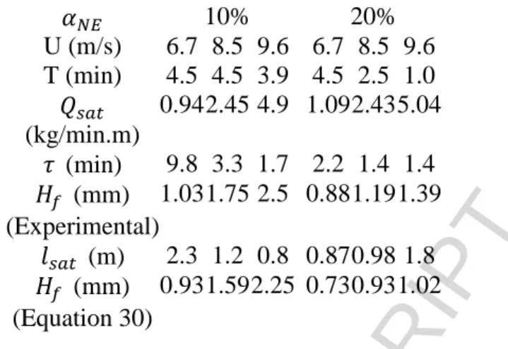
The values of 𝑙𝑠𝑎𝑡 and 𝐻𝑓 deduced from the above relationships are reported in Table 2 in comparison with the experimental values of the final eroded depth 𝐻𝑓 from the laser measurements. This provides fairly reasonable values.
ACCEPTED MANUSCRIPT
Table 2. Values of the saturation length 𝒍𝒔𝒂𝒕 and 𝑯𝒇 deduced from Equations 29-30 for the different sets of experiments. 𝛼𝑁𝐸 10% 20% U (m/s) 6.7 8.5 9.6 6.7 8.5 9.6 T (min) 4.5 4.5 3.9 4.5 2.5 1.0 𝑄𝑠𝑎𝑡 (kg/min.m) 0.94 2.45 4.9 1.09 2.43 5.04 𝜏 (min) 9.8 3.3 1.7 2.2 1.4 1.4 𝐻𝑓 (mm) (Experimental) 1.03 1.75 2.5 0.88 1.19 1.39 𝑙𝑠𝑎𝑡 (m) 2.3 1.2 0.8 0.87 0.98 1.8 𝐻𝑓 (mm) (Equation 30) 0.93 1.59 2.25 0.73 0.93 1.02
Fig. 10 presents the temporal evolution of the eroded depths of the sand bed obtained by laser measurements for two different cases. Notice that the erosion process is observed in the last part of the bed (between 5.50 𝑚 < 𝑥 < 5.82 m). Fig. 10(a) shows a sharp drop in the eroded depth (H) at 4 minutes and the pavement after 5 minutes. Fig. 10(b) shows similar behaviour but at different times. The same behaviour was observed in all tested cases, more or less sharply depending on the velocity and on 𝛼𝑁𝐸. These results enable a comprehension of how pavement occurs and are consistent with the results shown in Fig. 8. During the first minutes of the experiment, there were emissions along the whole tunnel. The eroded depth in the test section did not have significant changes since depositions also occurred. As the pavement phenomenon develops, initially at the beginning of the tunnel, emissions from the earlier portions decrease, tending to zero. At these moments, there would be no more deposition in the test section. Therefore, there is a sudden drop in the eroded depth, which corresponds to the stage when the pavement occurs at the part of the sand bed located in the test section (close to the end of the tunnel). As a consequence of the spatial differences on the temporal evolution of the eroded depth, it is difficult to estimate the emission rate using Equation 21, considering that there are laser measurements of a small part of the bed (320 mm, in the test section). Nonetheless, assuming that the final eroded depth is spatially constant, the emitted mass 𝐸𝑓 can be estimatedfrom laser measurements. Table 3 shows the experimental results of 𝐻𝑓 and the results of 𝐸𝑓 obtained from 𝐻𝑓 measurements and by weighing. The different procedures provide close values of 𝐸𝑓, demonstrating good measurement accuracy.
Figure 10. Temporal evolution of the eroded depths for two different cases: (a) 𝑼∞= 𝟗. 𝟔𝒎/𝒔 with 𝜶𝑵𝑬= 𝟏𝟎% and (b) 𝑼∞= 𝟖. 𝟓𝒎/𝒔 with 𝜶𝑵𝑬= 𝟐𝟎%
.
Table 3. Final eroded depths of the sand bed determined by laser methodology and estimated emitted mass obtained by 𝑯𝒇 measurements and by weighing
𝛼𝑁𝐸(%) 𝑈∞(𝑚/ 𝑠) 𝐻𝑓(𝑚𝑚) 𝐸(from 𝑓(𝑔) 𝐻𝑓) 𝐸𝑓(𝑔) (weighing) 10 6.7 1.03 2401.3 2393.3 8.5 1.75 4074.8 4140.9 9.6 2.5 5821.2 6095.2
ACCEPTED MANUSCRIPT
20 6.7 0.88 1821.4 1719.0 8.5 1.19 2461.0 2505.7 9.6 1.34 2773.5 3088.7
2. Final state of the particles bed after the pavement phenomenon
Fig. 11 presents pictures of the sand bed before and after the pavement for the simulated case with 𝑈∞= 8.5 𝑚/𝑠 and 𝛼𝑁𝐸 = 20%. Digital analysis of these photographs provided data of
final cover rates. The results are presented in Table 4.
Figure 11. Pictures of the sand bed (a) before and (b) after the pavement for 𝑼∞= 𝟖. 𝟓𝒎/𝒔 with 𝜶𝑵𝑬= 𝟐𝟎% Previous authors such as [12] have assumed that erosion ceases when the bed reaches a final cover rate independently of velocity and 𝛼𝑁𝐸. However, the results presented in Table 4 show that 𝐶𝑅𝑓 varies with 𝛼𝑁𝐸. In addition, the final cover rates and eroded depths of the sand bed
increase with velocity, as greater velocities cause more emissions and consequently greater accumulation of non-erodible particles.
For 𝛼𝑁𝐸 = 10% , the values of 𝐶𝑅𝑓 were lower than those found for 𝛼𝑁𝐸 = 20% . Nonetheless, the eroded depths are greater for 𝛼𝑁𝐸 = 10%. These results support the fact that the protective role of the non-erodible particles is not only given by the cover rate of the sand bed but also by the height of the non-erodible elements (see Equation 7).
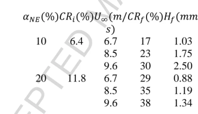
Table 4. Initial and final cover rates determined by digital analysis of photographs of the experiment and final eroded depths of the sand bed as determined by laser methodology (𝑯𝒇)
𝛼𝑁𝐸(%) 𝐶𝑅𝑖(%) 𝑈∞(𝑚/ 𝑠) 𝐶𝑅𝑓(%) 𝐻𝑓(𝑚𝑚) 10 6.4 6.7 17 1.03 8.5 23 1.75 9.6 30 2.50 20 11.8 6.7 29 0.88 8.5 35 1.19 9.6 38 1.34
Fig. 12 shows the ratio between 𝐶𝑅𝑓 and 𝐶𝑅𝑖 for each tested case. It can be seen that despite the lower values of 𝐶𝑅𝑓 for 𝛼𝑁𝐸= 10%, the increase in cover rate was proportionally more
steep. Moreover, the airflow velocity has more influence on the cover rate variation for the case with 𝛼𝑁𝐸 = 10%.
Figure 12. Variation of the cover rate for each tested configuration
5. Comparisons between model predictions and experiments
As explained in Section 3, the emitted mass is estimated by following three steps. (i) First, knowing the initial particle size distribution, the cover rate 𝐶𝑅 is written as a function of the eroded depth H (Equation 17). Fig. 13 presents 𝐶𝑅/𝐶𝑅𝑖 as a function of H obtained using Equation 17 (solid line) and the experimental data, which is the final state of the bed (𝐻𝑓 and 𝐶𝑅𝑓/𝐶𝑅𝑖) for each tested case (points). The formulation given by Equation 17 is well
supported by the experiments. (ii) Then, Equation 17 enables the calculation of the final eroded depth after the pavement phenomenon fora given velocity using Equation 19 (in the experimental configuration, 𝑢𝑀𝐼𝑁∗ = 𝑢𝑡∗𝑑(200𝜇𝑚) ≈ 0.186 𝑚/𝑠). It is important to state that
ACCEPTED MANUSCRIPT
both equations produce differences between the modelled and experimental results. Asa consequence, the propagated error of the final eroded depth leads to a variation in the emission estimation. (iii) Finally, emission is calculated using Equation 20.
Figure 13. Cover rate of non-erodible particles as a function of eroded depth obtained by modelling (Equation 17) and the values of 𝑯𝒇 and 𝑪𝑹𝒇/𝑪𝑹𝒊 obtained experimentally (Table 4)
Table 5 compares the estimated results of the final eroded depth (Equation 19) and the emitted mass with experimental data, including percentage errors. There is good agreement between the modelled and the experimental results for both measurements. The uncertainty of emission measurements, retrieved by previous repeatability tests with similar wind tunnel experiments, was found to be in the range of ±6.5%. Thus, the modelled results slightly underestimate the experimental data.
Table 5. Comparison of experimental and model results
𝛼𝑁𝐸 𝑈∞
(𝑚/ 𝑠)
𝐻𝑓 (mm) Emitted mass (g)
Exp. Mod. Error Exp. Mod. Error 10% 6.7 1.03 0.98 4.9% 2393.3 2345.1 2.0% 8.5 1.75 1.73 1.1% 4140.9 3802.9 8.2% 9.6 2.50 2.23 10.8% 6095.2 5231.8 14.2% 20% 6.7 0.88 0.50 43.2% 1719.0 1049.5 38.9% 8.5 1.19 0.99 16.8% 2505.7 2092.5 16.5% 9.6 1.34 1.26 6.0% 3088.7 2637.3 14.6%
The proposed model is a continuation of the work described in [12]. A limitation of the previous model is the assumption that erosion is finalised when the bed is completely overlaid by non-erodible particles. As explained in Section2, it has already been verified that erosion is terminated with a lower cover rate of the surface. Another limitation of the previous [12] model is related to the fact that the influence of saltation on transport is not accounted for. These two points have been adjusted in [12], but with a purely stochastic method that produces very large calculation times. On the other hand, the previous model has the advantage of providing detailed informationconcerning the temporal decrease of the emitted mass flux, although in practical cases such as fugitive sources on industrial sites, the most important information is the total emitted mass. Furthermore, the absolute value of the emitted mass is largely underestimated by the [12] model. The present study focused on modelling the final state of the bed after the pavement phenomenon and provides estimates of the global emissions, which are in good agreement with the experimental results. Moreover, it has the advantage of being represented by a simple mathematical expression.
6. Conclusion
This work investigated the pavement phenomenon and how it affects particle emissions from a bed of granular material exposed to a turbulent flow using experimental and analytical approaches. Wind erosion can lead to serious environmental impacts sincethe emissions can extend for large distance from the source. Literature review showed that dust emissions from diffuse sources are significant and may lead to air pollution episodes and consequently human healthy deterioration. Therefore, it is essential to have a proper emission model based on the physics of the phenomena and validated by experimental measurements.
The temporal evolution of the emitted mass flux revealed that during the first minutes, flux remained nearly constant, indicating that an equilibrium was established between wind flow
ACCEPTED MANUSCRIPT
and transport. The equilibrium state lasted longer for the lower velocities and for the beds with a lower proportion of non-erodible particles. After a few minutes, the flux began to decrease due to the pavement phenomenon. This decay was faster for higher velocities. In addition, greater amounts of non-erodible particles in the mixture led to a greater decay rate. These findings are consistent with previous studies in the literature [11,16].
A mathematical model for emitted mass estimates that includes the influence of the presence of non-erodible particles and saltation was proposed. The influence of saltation was included in the modelling using the dynamic threshold. The proportion of non-erodible particles on a bed surface after the pavement phenomenon was quantified. Although previous authors (e.g., [11,16]) have observed this phenomenon, it had not yet been quantified. Good agreement was found between the experimental and model results for the global emissions and bed eroded depth. Although the theory on which the proposed model is based is quite complex, the model is represented by a simple algebraic expression and demands low computational effort. Further work is still needed to improve the model for application to stockpiles of granular materials.
Acknowledgements
ACCEPTED MANUSCRIPT
References
[1] Alfaro, C., Gomes, L., 2001. Modeling mineral aerosol production by wind erosion : Emission intensities and aerosol size distributions in source areas. Journal of Geophysical Research 106, 75–84.
[2] Avecilla, F., Panebianco, J.E., Mendez, M.J., Buschiazzo, D.E., 2018. PM10 emission efficiency for agricultural soils: Comparing a wind tunnel, a dust generator, and the open-air plot. Aeolian Research 32, 116–123. doi:10.1016/j.aeolia.2018.02.003.
[3] Bagnold, R.A., 1941. The physics of blown sand and desert dunes. volume 265. Reprint ed., Methuen, London.
[4] Brown, S., Nickling, W.G., Gillies, J.A., 2008. A wind tunnel examination of shear stress partitioning for an assortment of surface roughness distributions. Journal of Geophysical Research: Earth Surface 113, 1–13. doi:10.1029/2007JF000790.
[5] Carvacho, O.F., Ashbaugh, L.L., Brown, M.S., Flocchini, R.G., 2004. Measurement of PM2.5 emission potential from soil using the UC Davis resuspension test chamber. Geomorphology 59, 75–80. doi:10.1016/j.geomorph.2003.09.007.
[6] Charru, F., Andreotti, B., Claudin, P., 2013. Sand Ripples and Dunes. Annual Review of Fluid Mechanics 45, 469–493. doi:10.1146/annurev-fluid-011212-140806.
[7] Chepil, W.S., 1945. Dynamics of wind erosion: I. Nature of movement of soil by wind. Soil Science 60, 305–320. doi:00010694-194510000-00004.
[8] Claudin, P., Andreotti, B., 2006. A scaling law for aeolian dunes on Mars, Venus, Earth, and for subaqueous ripples. Earth and Planetary Science Letters 252, 30–44. doi:10.1016/j.epsl.2006.09.004, arXiv:0603656.
[9] Courrech du Pont, S., 2015. Dune morphodynamics. Comptes Rendus Physique 16, 118– 138. doi:10.1016/j.crhy.2015.02.002.
[10] Crawley, D.M., Nickling, W.G., 2003. Drag partition for regularly-arrayed rough surfaces. Boundary-Layer Meteorology 107, 445–468. doi:10.1023/A:1022119909546, arXiv:arXiv:1011.1669v3.
[11] Descamps, I., 2004. Erosion éolienne d’un lit de particules à large spectre granulométrique. Wind erosion of a bed of particles with a wide size distribution. Ph.D. thesis. Ecole des Mines de Douai, Université de Valenciennes et du Hainaut-Cambrésis.
[12] Descamps, I., Harion, J.L., Baudoin, B., 2005. Taking-off model of particles with a wide size distribution . Chemical Engineering and Processing: Process Intensification 44, 159–166. doi:10.1016/j.cep.2004.04.007.
[13] Duan, S., Cheng, N., Xie, L., 2013. A new statistical model for threshold friction velocity of sand particle motion. CATENA 104, 32 – 38.
[14] Durán, O., Claudin, P., Andreotti, B., 2011. On aeolian transport: Grain-scale interactions, dynamical mechanisms and scaling laws. Aeolian Research 3, 243 – 270. doi:10.1016/j.aeolia.2011.07.006.
[15] Foucaut, J.M., Stanislas, M., 1996. Take-off threshold velocity of solid particles lying under a turbulent boundary layer. Experiments in Fluids 20, 377–382. doi:10.1007/BF00191019.
[16] Furieri, B., Harion, J., Milliez, M., Russeil, S., Santos, J., 2014a. Numerical modelling of aeolian erosion over a surface with non-uniformly distributed roughness elements. Earth Surface Processes and Landforms 39. doi:10.1002/esp.3435.
[17] Furieri, B., Russeil, S., Santos, J., Harion, J., 2013. Effects of non-erodible particles on aeolian erosion: Wind-tunnel simulations of a sand oblong storage pile. Atmospheric Environment 79, 672–680. doi:10.1016/j.atmosenv.2013.07.026.
ACCEPTED MANUSCRIPT
piles yards: Contribution of the surrounding areas. Environmental Fluid Mechanics 14, 51–67. doi:10.1007/s10652-013-9293-4.
[19] Gillette, D.A., Stockton, P.H., 1989. The effect of nonerodible particles on wind erosion of erodible surfaces. Journal of Geophysical Research: Atmospheres 94, 12885–12893. doi:10.1029/JD094iD10p12885.
[20] Hamdan, M.A., Refaat, A.A., Abdel Wahed, M., 2016. Morphologic characteristics and migration rate assessment of barchan dunes in the Southeastern Western Desert of Egypt. Geomorphology 257, 57–74. doi:10.1016/j.geomorph.2015.12.026.
[21] Ho, T.D., Valance, A., Dupont, P., Ould El Moctar, A., 2014. Aeolian sand transport: Length and height distributions of saltation trajectories. Aeolian Research 12, 65–74. doi:10.1016/j.aeolia.2013.11.004.
[22] Iversen, J.D., Rasmussen, K.R., 1994. The effect of surface slope on saltation threshold. Sedimentology 41, 721–728. doi:10.1111/j.1365-3091.1994.tb01419.x.
[23] Iversen, J.D., Wang, W.P., Rasmussen, K.R., Mikkelsen, H.E., Leach, R.N., 1991. Roughness element effect on local and universal saltation transport, in: Barndorff-Nielsen, O., Willetts, B. (Eds.), Aeolian Grain Transport. Springer Vienna. volume 2 of Acta Mechanica
Supplementum, pp. 65–75. doi:10.1007/978-3-7091-6703-8 5.
[24] Iversen, J.D., White, B.R., 1982. Saltation threshold on Earth, Mars and Venus. Sedimentology 29, 111–119. doi:10.1111/j.1365-3091.1982.tb01713.x.
[25] Kheirabadi, H., Mahmoodabadi, M., Jalali, V., Naghavi, H., 2018. Sediment flux, wind erosion and net erosion influenced by soil bed length, wind velocity and aggregate size distribution. Geoderma 323, 22–30. doi:10.1016/j.geoderma.2018.02.042.
[26] Kok, J., Renno, N., 2006. Enhancement of the emission of mineral dust aerosols by electric forces. Geophysical research letters 33, 1–5. doi:10.1029/2006GL026284.
[27] Kok, J.F., Parteli, E.J.R., Michaels, T.I., Karam, D.B., 2012. The physics of wind-blown sand and dust. Reports on Progress in Physics 75, 106901. doi:10.1088/0034-4885/75/10/106901.
[28] Kok, J.F., Renno, N.O., 2009. A comprehensive numerical model of steady state saltation (COMSALT). Journal of Geophysical Research: Atmospheres 114, 1–20. doi:10.1029/2009JD011702.
[29] Li, B., McKenna Neuman, C., 2014. A wind tunnel study of aeolian sediment transport response to unsteady winds. Geomorphology 214, 261–269. doi:10.1016/j.geomorph.2014.02.010.
[30] Li, L., Martz, L.W., 1995. Aerodynamic dislodgement of multiple-size sand grains over time. Sedimentology 42, 683–694. doi:10.1111/j.1365-3091.1995.tb00400.x.
[31] Lima, I.A., Araújo, A.D., Parteli, E.J., Andrade, J.S., Herrmann, H.J., 2017. Optimal array of sand fences. Scientific Reports 7, 1–8. doi:10.1038/srep45148.
[32] Liu, L.Y., Shi, P.J., Zou, X.Y., Gao, S.Y., Erdon, H., Yan, P., Li, X.Y., Dong, Z.B., Wang, J.H., 2003. Short-term dynamics of wind erosion of three newly cultivated grassland soils in Northern China . Geoderma 115, 55 – 64. doi:10.1016/S0016-7061(03)00075-2. [33] Lyles, L., Schrandt, R.L., Schmeidler, N.F., 1974. How aerodynamic roughness elements control sand movement. Transactions of the American Society for Agricultural Engineers 17, 134–139. doi:10.13031/2013.36805.
[34] Marshall, J.K., 1971. Drag measurements in roughness arrays of varying density and distribution. Agricultural Meteorology 8, 269–292. doi:10.1016/0002-1571(71)90116-6. [35] Marticorena, B., Bergametti, G., 1995. Modeling the atmospheric dust cycle: 1. Design of a soil-derived dust emission scheme. Journal of Geophysical Research: Atmospheres 100, 16415–16430. doi:10.1029/95JD00690.
[36] Martin, R.L., Kok, J.F., Hugenholtz, C.H., Barchyn, T.E., Chamecki, M., Ellis, J.T., 2018. High-frequency measurements of aeolian saltation flux: Field-based methodology and
ACCEPTED MANUSCRIPT
applications. Aeolian Research 30, 97–114. doi:10.1016/J.AEOLIA.2017.12.003.
[37] Mayaud, J.R., Bailey, R.M., Wiggs, G.F., Weaver, C.M., 2017. Modelling aeolian sand transport using a dynamic mass balancing approach. Geomorphology 280, 108–121. doi:10.1016/j.geomorph.2016.12.006.
[38] McKenna Neuman, C., Sanderson, R.S., Sutton, S., 2013. Vortex shedding and morphodynamic response of bed surfaces containing non-erodible roughness elements. Geomorphology 198, 45–56. doi:10.1016/j.geomorph.2013.05.011.
[39] Musick, H.B., Trujillo, S.M., Truman, C.R., 1996. Wind-tunnel modelling of the influence of vegetation structure on saltation threshold. Earth Surface Processes and
Landforms 21, 589–605.
doi:10.1002/(SICI)1096-9837(199607)21:7<589::AID-ESP659>3.0.CO;2- 1.
[40] Neuman, C.M., Bédard, O., 2015. Journal of Geophysical Research : Earth Surface , 1– 17doi:10.1002/2015JF003475.Received.
[41] Nickling, W.G., Neuman, C.M., 2009. Aeolian sediment transport, in: Parsons, A., Abrahams, A. (Eds.), Geomorphology of Desert Environments. Springer, pp. 517–555. doi:10.1007/978-1-4020-5719-9 17.
[42] Raffaele, L., Bruno, L., Wiggs, G.F., 2018. Uncertainty propagation in aeolian processes: From threshold shear velocity to sand transport rate. Geomorphology 301, 28–38. doi:10.1016/j.geomorph.2017.10.028.
[43] Raupach, M.R., 1992. Drag and drag partition on rough surfaces. Boundary-Layer Meteorology 60, 375–395. doi:10.1007/BF00155203.
[44] Raupach, M.R., Gillette, D.A., Leys, J.F., 1993. The effect of roughness elements on wind erosion threshold. Journal of Geophysical Research: Atmospheres 98, 3023–3029. doi:10.1029/92JD01922.
[45] Schlichting, H., 1936. Experimentelle Untersuchungen zum Rauhigkeitsproblem. Ingenieur-Archiv 7, 1–34. doi:10.1007/BF02084166.
[46] Seinfeld, J.H., Pandis, S.N., 2006. Atmospheric Chemistry and Physics: from Air Pollution to Climate Change. volume 51. Second ed., John Wiley & Sons, Inc. doi:10.1016/0016-7037(87)90252-3.
[47] Shao, Y., Lu, H., Shag, Y., 2000. A simple expression for wind erosion threshold friction velocity. Journal of Geophysical Research 105, 22437–22443. doi:https://doi.org/10.1029/2000JD900304.
[48] Smith, I.B., Spiga, A., Holt, J.W., 2015. Aeolian processes as drivers of landform evolution at the South Pole of Mars. Geomorphology 240, 54–69. doi:10.1016/j.geomorph.2014.08.026.
[49] Swet, N., Katra, I., 2016. Reduction in soil aggregation in response to dust emission processes. Geomorphology 268, 177–183. doi:10.1016/j.geomorph.2016.06.002.
[50] Turpin, C., Badr, T., Harion, J.L., 2010. Numerical modelling of aeolian erosion over rough surfaces. Earth Surface Processes and Landforms 35, 1418–1429. doi:10.1002/esp.1980. [51] Turpin, C., Harion, J.L., 2009. Numerical modeling of flow structures over various flat-topped stockpiles height: Implications on dust emissions. Atmospheric Environment 43, 5579 – 5587. doi:10.1016/j.atmosenv.2009.07.047.
[52] Walter, B., Gromke, C., Lehning, M., 2012. Shear-Stress Partitioning in Live Plant Canopies and Modifications to Raupach’s Model. Boundary-Layer Meteorology 144, 217– 241. doi:10.1007/s10546-012-9719-4.
[53] Webb, N.P., Galloza, M.S., Zobeck, T.M., Herrick, J.E., 2016. Threshold wind velocity dynamics as a driver of aeolian sediment mass flux. Aeolian Research 20, 45–58. doi:10.1016/j.aeolia.2015.11.006.
[54] Webb, N.P., Strong, C.L., 2011. Soil erodibility dynamics and its representation for wind erosion and dust emission models. Aeolian Research 3, 165–179.
ACCEPTED MANUSCRIPT
doi:10.1016/j.aeolia.2011.03.002.
[55] WHO, 2006. The World Health Report. Technical Report. World Health Organization. [56] Wolfe, S.A., Nickling, W.G., 1996. Shear stress partitioning in sparsely vegetated desert canopies. Earth Surface Processes and Landforms 21, 607–619. doi:10.1002/(SICI)1096-9837(199607)21:7<607::AID-ESP660>3.0.CO;2- 1.
[57] Yang, F., Yang, X.H., Huo, W., Ali, M., Zheng, X.Q., Zhou, C.L., He, Q., 2017. A continuously weighing, high frequency sand trap: Wind tunnel and field evaluations. Geomorphology 293, 84–92. doi:10.1016/j.geomorph.2017.04.008.
[58] Zobeck, T.M., Sterk, G., Funk, R., Rajot, J.L., Stout, J.E., Van Pelt, R.S., 2003. Measurement and data analysis methods for field-scale wind erosion studies and model validation. Earth Surface Processes and Landforms 28, 1163–1188. doi:10.1002/esp.1033.