Feedback generation of quantum Fock states by discrete QND measures

HAL Id: hal-00485694

https://hal-mines-paristech.archives-ouvertes.fr/hal-00485694

Submitted on 21 May 2010

HAL is a multi-disciplinary open access

archive for the deposit and dissemination of

sci-entific research documents, whether they are

pub-lished or not. The documents may come from

teaching and research institutions in France or

abroad, or from public or private research centers.

L’archive ouverte pluridisciplinaire HAL, est

destinée au dépôt et à la diffusion de documents

scientifiques de niveau recherche, publiés ou non,

émanant des établissements d’enseignement et de

recherche français ou étrangers, des laboratoires

publics ou privés.

Feedback generation of quantum Fock states by discrete

QND measures

Mazyar Mirrahimi, Igor Dotsenko, Pierre Rouchon

To cite this version:

Mazyar Mirrahimi, Igor Dotsenko, Pierre Rouchon. Feedback generation of quantum Fock states by

discrete QND measures. 48th IEEE Conference on Decision and Control, Dec 2009, Shanghai, China.

pp.1451 - 1456, �10.1109/CDC.2009.5399839�. �hal-00485694�

arXiv:0903.0996v2 [quant-ph] 4 May 2009

Feedback generation of quantum Fock states by discrete QND measures

Mazyar Mirrahimi, Igor Dotsenko and Pierre Rouchon

Abstract— A feedback scheme for preparation of photon number states in a microwave cavity is proposed. Quantum Non Demolition (QND) measurement of the cavity field provides information on its actual state. The control consists in injecting into the cavity mode a microwave pulse adjusted to increase the population of the desired target photon number. In the ideal case (perfect cavity and measures), we present the feedback scheme and its detailed convergence proof through stochastic Lyapunov techniques based on super-martingales and other probabilistic arguments. Quantum Monte-Carlo simulations performed with experimental parameters illustrate convergence and robustness of such feedback scheme.

I. INTRODUCTION

In [10], [5], [4] QND measures are exploited to detect and/or produce highly non-classical states of light trapped in a super-conducting cavity (see [6, chapter 5] for a description of such QED systems and [1] for detailed physical models with QND measures of light using atoms). For such experi-mental setups, we detail and analyze here a feedback scheme that stabilize the cavity field towards any photon-number states (Fock states). Such states are strongly non-classical since their photon numbers are perfectly defined. The control corresponds to a coherent light-pulse injected inside the cavity between atom passages. The overall structure of the proposed feedback scheme is inspired of [3] using a quantum adaptation of the observer/controller structure widely used for classical systems (see, e.g., [7, chapter 4]). The observer part of the proposed feedback scheme consists in a discrete-time quantum filter, based on the observed detector clicks, to estimate the quantum-state of the cavity field. This estimated state is then used in a state-feedback based on Lyapunov design, the controller part. In theorems 1 and 2 we prove the convergence almost surely of the closed-loop system towards the goal Fock-state in absence of modeling imperfections and measurement errors. Simulations illustrate this results and show that performance of the closed-loop system are not dramatically changed by false detections for 10% of the detector clicks. In [2] similar feedback schemes are also addressed with modified quantum filters in order to take into account additional physical effects and experimental imperfections. [2] focuses on physics and includes extensive

This work was supported in part by the ”Agence Nationale de la Recherche” (ANR), Projet Blanc CQUID number 06-3-13957.

M. Mirrahimi is with INRIA Rocquencourt, Domaine de Voluceau, B.P. 105, 78153 Le Chesnay cedex, France,

mazyar.mirrahimi@inria.fr

I. Dotsenko is with Laboratoire Kastler Brossel, ´Ecole Normale Sup´erieure, CNRS, Universit´e P. et M. Curie, 24 rue Lhomond, F-75231 Paris Cedex 05, Franceigor.dotsenko@lkb.ens.fr

P. Rouchon is with Mines ParisTech, Centre Automatique et Syst`emes, Math´ematiques et Syst`emes, 60 Bd Saint Michel, 75272 Paris cedex 06, France,pierre.rouchon@mines-paristech.fr

closed-loop simulations whereas here we are interested by mathematical aspects and convergence proofs.

In section II, we describe very briefly the physical system and its quantum Monte-Carlo model. In section III the feed-back is designed using Lyapunov techniques. Its convergence is proved in theorem 1. Section IV introduces a quantum filter to estimate the cavity state necessary for the feedback: convergence of the closed-loop system (quantum filter and feedback based on the estimate cavity state) is proved in theorem 2 assuming perfect model and detection.This section ends with Theorem 3 proving a contraction property of the quantum filter dynamics. Section V is devoted to closed-loop simulations where measurement imperfections are introduced for testing robustness.

The authors thank Michel Brune, Serge Haroche and Jean-Pierre Raimond for useful discussions and advices.

II. THE PHYSICAL SYSTEM AND ITS JUMP DYNAMICS

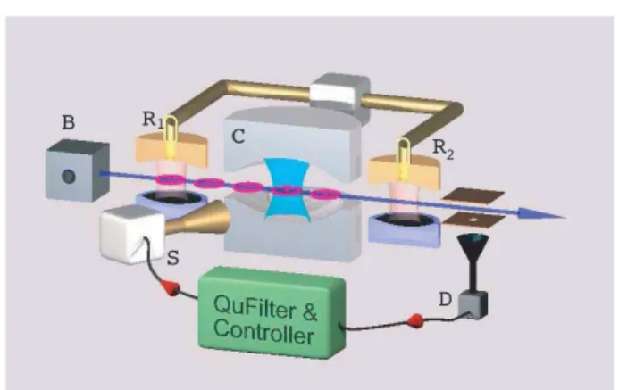
B _C

D S

R 1

R ₂

Fig. 1. The microwave cavity QED setup with its feedback scheme (in green).

As illustrated by figure 1, the system consists in C a high-Q microwave cavity, in B a box producing Rydberg

atoms, in R1 and R2 two low-Q Ramsey cavities, in D an

atom detector and in S a microwave source. The dynamics model is discrete in time and relies on quantum Monte-Carlo trajectories (see [6, chapter 4]). It takes into account the back-action of the measure. It is adapted from [5] where we have just added the control effect.

Each time-step indexed by the integer k corresponds to atom number k coming from B, submitted then to a first

Ramsey π/2-pulse in R1, crossing the cavity C and being

entangled with it, submitted to a second π/2-pulse in R2

and finally being measured in D. The state of the cavity

is described by the density operator ρk. Here the passage

measurement of the cavity state, by detecting the state of the

Rydberg atom number k after leaving R2. During this same

step, an appropriate coherent pulse (the control) is injected into C. Denoting, as usual, by a the photon annihilation

operator and by N = a†_{a the photon number operator, the}

density matrix ρk+1 is related to ρk through the following

jump-relationships: ρk+1=

D(αk)MkρkMk†D(−αk)

Tr₍MkρkMk†)

where

• the measurement operator Mk = Mg(resp. Mk = Me),

when the atom k is detected in the state |g! (resp. |e!) with Mg = cos „ φR+ φ 2 + N φ « , Me= sin „ φR+ φ 2 + N φ « . (1)

Such measurement process corresponds to an off-resonant interaction between atom k and cavity where

φRis the direction of the second Ramsey π/2-pulse (R2

in figure 1) and φ is the de-phasing-angle per photon.

• The probability Pg,k (resp. Pe,k) of detecting the atom

k in |g! (resp. |e!) is given by Tr (MgρkMg) (resp.

Tr (MeρkMe).

• D(αk) is the displacement operator describing the

co-herent pulse injection, D(αk) = exp(αk(a†− a)), and

the scalar control αk is a real parameter that can be

adjusted at each time step k.

The time evolution of the step k to k + 1, in fact, consists of two types of evolutions: a projective measurement and a coherent injection. For simplicity sakes, we will use

the notation of ρk+1

2, to illustrate this intermediate step.

Therefore, ρ_k+1 2 = MkρkMk† Tr“MkρkM_k† ” , ρk+1= D(αk)ρk+1 2 D_(−αk) (2)

In the sequel, we consider the finite dimensional

approx-imation defined by a maximum of photon number, nmax_{. In}

the truncated Fock basis (|n!)0≤n≤nmax, N corresponds to

the diagonal matrix (diag(n))_0≤n≤nmax, ρ is a (nmax+ 1) ×

(nmax_{+ 1) symmetric positive matrix with unit trace, and}

the annihilation operator a is an upper-triagular matrix with (√n)1≤n≤nmax as upper diagonal, the remaining elements

being 0. We restrict to real quantities since the phase of any Fock state is arbitrary. We set it here to 0.

III. FEEDBACK SCHEME AND CONVERGENCE PROOF

We aim to stabilize the Fock state with ¯n photons

char-acterized by the density operator ¯ρ = |¯n! %¯n|. To this end

we choose the coherent feedback αk such that the value of

the Lyapunov function V (ρ) = 1 − Tr (ρ¯ρ) decreases when

passing from ρk+1

2 to ρk+1. Note that, for α small enough,

the Baker-Campbell-Hausdorff formula yields the following approximation D_{(α)ρD(−α) ≈ ρ − α[ρ, a}†_{− a] +}α 2 2 [[ρ, a † − a], a†− a] (3)

up to third order terms. Therefore, for αksmall enough, we

have Tr“D(αk)ρ_k+1 2D(−αk)¯ρ ” = Tr“ρ_k+1 2ρ¯ ” − αkTr “ [ρ_k+1 2, a † − a]¯ρ ” +α 2 k 2 Tr “ [[ρ_k+1 2, a † − a], a†− a]¯ρ”.

Thus the feedback

αk = c1Tr ! [¯ρ, a†_{− a]ρ} k+1 2 " (4)

with a gain c1> 0 small enough ensures that

Tr (¯ρρk+1) − Tr “ ¯ ρρ_k+1 2 ” ≥c₂1˛˛ ˛Tr “ [¯ρ, a†− a]ρk+1₂ ” ˛ ˛ ˛ 2 , (5) since Tr![ρk+1 2, a †_{− a]¯ρ}"_{= −Tr}!_{[¯ρ, a}†_{− a]ρ} k+1 2 " .

Fur-thermore, the conditional expectation of Tr!ρρ¯ k+1

2 " know-ing ρk is given by

E

“Tr“ρρ¯ _k+1 2 ” | ρk ” = Pg,kTr ¯ ρMgρkMg† Pg,k ! + Pe,kTr „ ¯ρMeρkMe† Pe,k « = Tr (¯ρρk) since [¯ρ, Mg] = [¯ρ, Me] = 0 and Mg†Mg + Me†Me = 11. Thus

E

(Tr (¯ρρk+1) | ρk) ≥

E

! Tr!ρρ¯ k+1 2 " | ρk " = Tr (¯ρρk)

and consequently, the expectation value of V (ρk) decreases

at each sampling time:

E

(V (ρk+1)) ≤

E

(V (ρk)) . (6)

Considering the Markov process ρk, we have therefore shown

that V (ρk) is a super-martingale bounded from below by 0.

When V reaches its minimum 0, the Markov process ρk

has converged to ¯ρ. However, one can easily see that this

super-martingale has also the possibility to converge towards other attractors, for instance other Fock states which are all the stationary points of the closed-loop Markov process but with V (ρ) = 1 instead of 0. Following [9], we suggest the following modification of the feedback scheme:

αk= 8 > < > : c1Tr “ [¯ρ, a†_{− a]ρ} k+1 2 ” if V (ρk) ≤ 1 − ε argmax α∈[− ¯α,¯α] Tr“ρD(α)ρ¯ _k+1 2D(−α) ” if V (ρk) > 1 − ε (7) with c1, ε, ¯α > 0 constants.

Theorem 1: Consider (2) and assume that for all n ∈

{0, . . . , nmax

} we have φR+φ

2 + nφ )= 0 mod (π/2) and that

#  cos2„ φR+ φ 2 + nφ « | n ∈ {0, . . . , nmax } ff = nmax + 1.

Take the switching feedback scheme (7) with ¯α > 0. For

small enough c1 > 0 and ε > 0, the trajectories of (2)

converge almost surely towards the target Fock state ¯ρ.

Remark 1: The second part of the feedback (7), dealing

with states near the bad attractors, is not explicit and may seem hard to compute. Note that, this form has been partic-ularly chosen to simplify the proof of the Theorem 1 and

in practice, one can take it to be any constant control field exciting the system around these bad attractors and ensuring a fast return to the inner set.

Remark 2: The controller gain c1 can be tuned

in order to maximize at each sampling time k,

Tr!D(αk)ρk+1

2D(−αk)¯ρ

"

for ρk+1

2 near ¯ρ. Up to

third order term in ρk+1

2 − ¯ρ, (3) yields to Tr“D(αk)ρ_k+1 2 D_(−αk)¯ρ ” = Tr“ρρ¯ _k+1 2 ” + “ Tr“[¯ρ, a†− a]ρk+1 2 ””2„ c1− c21 2Tr “ [¯ρ, a†− a][¯ρ, a†− a]” « .

Thus c1 = 1/Tr#[¯ρ, a†− a][¯ρ, a†− a]$ ≈ 1/(4¯n + 2) for

nmax_{+ ¯n implies a maximum decrease at the sampling time,}

up to third-order terms in ρk− ¯ρ.

In order to prove the Theorem 1, we need some classical tools from stochastic processes namely the Doob’s inequality and the Kushner’s asymptotic invariance Theorem [8]. These results are been recalled in the Appendix.

Proof of Theorem 1. It is divided in 3 steps: in a first

step, we show that for small enough ε and by applying the second part of the feedback scheme, the trajectories starting within the set {ρ | V (ρ) > 1 − ε} reach in one step the set {ρ | V (ρ) ≤ 1 − 2ε} and this with probability 1; next, we show that trajectories starting within the set {ρ | V (ρ) ≤ 1 − 2ε}, will never hit the set {ρ | V (ρ) > 1 − ε} with a uniformly non-zero probability p > 0; finally, we will show

that, the trajectories of the quantum filter converge towards ¯ρ

for almost all trajectories that never hit the set {ρ | V (ρ) > 1 − ε}. This is then an immediate conclusion of the Markov property that the trajectories of the quantum filter with the

feedback scheme (7) will converge almost surely towards ¯ρ.

Step 1: We start by considering the process starting on the level set {ρ | V (ρ) = 1}. We have the following lemma:

Lemma 1: Consider ρ a well-defined density matrix such

that Tr (ρ¯ρ) = 0. We have min s∈{g,e}α∈[− ¯maxα,¯α] Tr` ¯ρD(α)MsρMs†D(−α) ´ Tr“MsρMs† ” >0.

We denote any argument of the above min-max problem by ¯

α(ρ) ∈ [−¯α, ¯α].

Proof of Lemma 1: Define ρs = MsρM

† s

Tr₍MsρMs†), s ∈ {g, e}.

The matrices Mg and Me being diagonal, we trivially have

Tr (ρsρ) = 0. Let us fix s and assume that for all α ∈¯

[−¯α, ¯α],

Tr (¯ρD(α)ρsD(−α)) = 0. (8)

Decomposing ρs as a sum of projectors we have ρs =

%m

k=1λk,s|ψk,s! %ψk,s| , where λk,s are strictly positive

eigenvalues and ψk,s are the associated normalized

eigen-states of ρs (m = 1 corresponds to the case where ρs is a

projector). The equation (8), clearly, implies

&ψk,s | D(−α)¯n' = 0, ∀k ∈ {1, · · · , m}, ∀α ∈ [−¯α,α]. (9)¯

Fixing one k ∈ {1, · · · , m} and taking ψ = ψk,s, noting

that D(−α) = exp(−α(a†_{− a)) and deriving j times versus}

α around 0 we get

&ψ | (a†_{− a)}j_{n' = 0,¯ ∀j = 0, . . . , n}max

. (10)

But the family #(a†_{− a)}j_¯n$

0≤j≤nmax is full rank. This is a

direct consequence of [11, Theorem 4]. It is proved there that

the truncated harmonic oscillator d

dt|φ!t= −(ıN +v(t)(a†−

a)) |φ!t, is completely controllable with the single scalar

control v(t). If the rank r of #(a†_{− a)}p_|¯n!$

0≤p≤nmax is

strictly less that nmax_{+ 1, then according to Cayley-Hamilton}

Theorem the rank of the infinite family#(a†_{− a)}p_|¯n!$

p≥0

is also r. Take |ξ!, a state orthogonal to this family. For

any control v(t), the state |φ!t starting from |¯n! remains

orthogonal to |ξ!. Thus it will be impossible to find a control

v(t) steering |φ!t from |¯n! to |ξ!.

Since the rank of #(a†_{− a)}p_|¯n!$

0≤p≤nmax is maximum,

(10) implies |ψk! = 0 and leads to a contradiction. !

Applying the compactness of the space of density matri-ces, we directly have the following corollary:

Corollary 1: There exists an ) > 0 such that

inf ρ∈{Tr(ρ ¯ρ)<#} Tr` ¯ρD( ¯α(ρ))MsρMs†D(−¯α(ρ)) ´ Tr“MsρMs† ” >2& (11)

for s = g, e and where ¯α(ρ) is defined in Lemma 1.

Proof of Corollary 1: We take

δ= inf ρ∈{Tr(ρ ¯ρ)=0}s∈{g,e}min Tr` ¯ρD( ¯α(ρ))MsρMs†D(−¯α(ρ)) ´ Tr“MsρMs† ” .

By Lemma 1 and the compactness of the set {ρ | Tr (ρ¯ρ) =

0}, we know that δ > 0. By continuity of Tr (ρ¯ρ) with respect

to ρ and by compactness of the space of density matrices, there exists γ > 0 such that

inf ρ∈{Tr(ρ ¯ρ)<γ}s∈{g,e}min Tr` ¯ρD( ¯α(ρ))MsρMs†D(−¯α(ρ)) ´ Tr“MsρMs† ” > δ 2.

Therefore, by taking ) = min(γ, δ/4), clearly, (11) holds true. !

Through this corollary, we have shown that whenever the

Markov process hits the set {Tr (ρ¯ρ) < )}, it is immediately

rebounded to the set {Tr (ρ¯ρ) > 2)} and this with

probabil-ity 1.

Step 2: Let us assume that the process starts within the

set {Tr (ρ¯ρ) > 2)}.

Lemma 2: Initializing the Markov process within the set

{ρ | V (ρ) ≤ 1 − 2)}, ρk will never hit the set {ρ | V (ρ) >

1 − )} with a probability p > $

1−$ > 0.

Proof of Lemma 2: By (6), the process V (ρk) is, clearly, a

supermartingale. One only needs to use the Doobs inequality (cf. Appendix, Theorem 4) and we have

P( sup 0≤k<∞ V(ρk) > 1 − &) < V(ρ0) 1 − & ≤ 1 − 2& 1 − & , and thus p > 1 − (1 − 2))/(1 − )) = )/(1 − )). !

We have shown that starting within the inner set

{Tr (ρ¯ρ) ≥ 2)} there is a uniform non-zero probability

of )/(1 − )) for the process, to never hit the outer set

{Tr (ρ¯ρ) < )}.

Step 3:

Lemma 3: The sample paths ρk remaining into the set

Proof of Lemma 3: Consider the function W(ρ) = 1 − Tr (ρ¯ρ)2. For s = g, e, set ρs= MsρM † s Tr(MsρMs†). We have W(ρg) = 1 − Tr`ρM† gρM¯ g´ 2 Tr“MgρMg† ”2, = 1 − ˛ ˛ ˛ cos “ φR+φ 2 + ¯nφ ” ˛ ˛ ˛ 4 Tr“MgρMg† ”2 Tr (ρ¯ρ) 2 , (12) and similarly W(ρe) = 1 − ˛ ˛ ˛ sin “ φR+φ 2 + ¯nφ ” ˛ ˛ ˛ 4 Tr“MeρMe† ”2 Tr (ρ¯ρ) 2 . (13)

Furthermore, whenever α is given by the first part of the feedback law, we have

W(D(α)ρD(−α)) − W(ρ) ≤ −2&c1 ˛ ˛ ˛Tr “ [¯ρ, a†− a]ρ” ˛˛ ˛ 2 , (14)

where we have applied (5) together with the fact that

|Tr (D(α)ρD(−α)¯ρ) | + |Tr (ρ¯ρ) | ≥ 2)

since ρ is inside the set {Tr (ρ¯ρ) > )}.

Apply-ing (2), (12), (13) and (14) for the paths never leavApply-ing the

set {Tr (ρ¯ρ) > )}, we have

E

(W(ρk+1) | ρk) − W(ρk) ≤ −2"c1 ˛ ˛ ˛Tr “ [¯ρ, a†− a]ρ_k+1 2 ” ˛ ˛ ˛ 2 − 0 @ ˛ ˛ ˛ cos “ φR+φ 2 + ¯nφ ” |4 Tr“MgρkMg† ” + ˛ ˛ ˛ sin “ φR+φ 2 + ¯nφ ” |4 Tr“MeρkMe† ” − 1 1 ATr (ρkρ)¯2. Noting thatTr#MgρkMg† $ ≥ 0, Tr#MeρkMe† $ ≥ 0, Tr#MgρkMg† $ + Tr#MeρkMe† $ = 1 and by Cauchy-Schwartz inequality, we have

˛ ˛ ˛ cos “ φR+φ 2 + ¯nφ ” ˛ ˛ ˛ 4 Tr“MgρkMg† ” + ˛ ˛ ˛ sin “ φR+φ 2 + ¯nφ ” ˛ ˛ ˛ 4 Tr“MeρkMe† ” = 0 B @ ˛ ˛ ˛ cos “ φ_R+φ 2 + ¯nφ ” ˛ ˛ ˛ 4 Tr“MgρkMg† ” + ˛ ˛ ˛ sin “ φ_R+φ 2 + ¯nφ ” ˛ ˛ ˛ 4 Tr“MeρkMe† ” 1 C A (Tr“MgρkMg† ” + Tr“MeρkMe† ” ) ≥ „ cos2„ φR+ φ 2 + ¯nφ « + sin2„ φR+ φ 2 + ¯nφ ««2 = 1,

with equality if and only if Tr#MgρkMg†

$ =

cos2!φR+φ

2 + ¯nφ

"

. We apply, now, the Kushner’s invari-ance Theorem (cf. Appendix, Theorem 5) to the Markov

process ρk with the Lyapunov function W(ρk). The process

ρk converges in probability to the largest invariant set

in-cluded in ( ρ | Tr#MgρMg†$ = cos 2) φR+ φ 2 + ¯nφ * + , -ρ | Tr #[¯ρ, a†_{− a]M} sρMs†$ = 0, s = g, e. .

In particular, by invariance, ρ belonging to this limit set

implies Tr#MgρMg†

$

= Tr(MgMsρMs†Mg†)

Tr₍MsρMs†) for s = g, e.

Taking s = g, and noting that Mg = Mg†, this leads to

Tr#M4 gρ $ = Tr#M2 gρ $2 . However, by Cauchy-Schwartz inequality, and applying the fact that ρ is a positive matrix,

we have Tr#M4

gρ$ = Tr #Mg4ρ$ Tr (ρ) ≥ Tr #Mg2ρ

$2

, with

equality if and only if M4

gρ and ρ are co-linear. Since Mg4has

a non degenerate spectrum, ρ is necessarily a projector over

one of the eigen-state of M4

g, i.e., a Fock state |n!, for some

n ∈ {0, . . . , nmax

}. Finally, as we have restricted ourselves to

the paths never leaving the set {ρ | Tr (ρ¯ρ) > )}, the only

possibility for the invariant set is the isolated point {¯ρ}. !

Lemma 4: ρk converges to ¯ρ for almost all paths

remain-ing in the set {Tr (ρ¯ρ) > )}.

Proof of Lemma 4: Define the event P>$ =

{ω ∈ Ω | ρk never leaves the set {Tr (ρ¯ρ) >

)}}. Through Lemma 3, we have shown that

limk→∞

P

(/ρk− ¯ρ/ > δ | P>$) = 0, ∀δ > 0. By

continuity of V (ρ) = 1 − Tr (ρ¯ρ), this also implies that

limk→∞

P

(V (ρk) > δ | P>$) = 0, ∀δ > 0. As V (ρ) ≤ 1,

we have

E

(V (ρk) | P>$) ≤

P

(V (ρk) > δ | P>$)

+ δ(1 −

P

(V (ρk) > δ | P>$)).

Thus lim supk→∞

E

(V (ρk) | P>$) ≤ δ, ∀δ > 0, and

so limk→∞

E

(V (ρk) | P>$) = 0. By Theorem 4, we

know that V (ρk) converges almost surely and therefore,

as V is bounded, by dominated convergence, we obtain

E

(limk→∞V (ρk) | P>$) = 0.!

Now, we have all the elements to finish the proof of the Theorem 1. From Steps 1 and 2 and the Markov property, one

deduces that for almost all paths ρk, there exists a ¯K such

that ρk for k ≥ ¯K never leaves the set {Tr (ρ¯ρ) > )}. This

together with the step 3 finishes the proof of the Theorem.!

IV. QUANTUM FILTERING FOR STATE ESTIMATION

The feedback law (7) requires the knowledge of ρk+1

2.

When the measurement process is fully efficient and the jump model (2) admits no error, it actually represents a natural

choice for quantum filter to estimate the value of ρ by ρest

satisfying ρest k+1= D(αk)ρestk+1 2D(−αk) ρest k+1 2 = Mskρ est kMs†k Tr!Mskρ est kM † sk " . (15)

where sk = g or e, depending on measure outcome k and

on the control αk.

Before passing to the parametric robustness of the feed-back scheme, let us discuss the robustness with respect to the choice of the initial state for the filter equation

when we replace ρk+1

2 by ρ est

k+1

2 in the feedback (7). Note

that, Theorem 1 shows that whenever the filter equation is initialized at the same state as the one which the physical system is prepared initially, the feedback law ensures the stabilization of the target state. The next theorem shows that as soon as the quantum filter is initialized at any arbitrary fully mixed initial state (not necessarily the same as the initial

state of the physical system (2)) and whenever the feedback scheme (7) is applied on the system, the state of the physical system will converge almost surely to the desired Fock state.

Theorem 2: Assume that the quantum filter (15) is

initial-ized at a full-rank matrix ρest

0 and that the feedback scheme (7)

is applied to the physical system. The trajectories of the system (2), will then converge almost surely to the target

Fock state ¯ρ.

Proof of Theorem 2: The initial state ρest

0 being full-rank,

there exists a γ > 0 such that ρest

0 = γρ0+ (1 − γ)ρc0, where

ρ0 is the initial state of (2) at which the physical system

is initially prepared and ρc

0 is a well-defined density matrix.

Indeed, ρest _{being positive and full-rank, for a small enough}

γ, (ρest

0− γρ0)/(1 − γ) remains non-negative, Hermitian and

of unit trace.

Assume that, we prepare the initial state of another identi-cal physiidenti-cal system as follows: we generate a random number r in the interval (0, 1); if r < γ we prepare the system in

the state ρ0 and otherwise we prepare it at ρc0. Applying

our quantum filter (15) (initialized at ρest

0) and the associated

feedback scheme, almost all trajectories of this physical

system converge to the Fock state ¯ρ. In particular, almost

all trajectories that were initialized at the state ρ0 converge

to ¯ρ. This finishes the proof of the theorem. !

The quantum filter (15) admits also some contraction properties confirming its robustness to experimental errors as shown by simulations of figures 3 and 4 where detection errors are introduced. We just provide here a first interesting inequality that will be used in future developments.

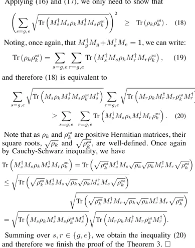
Theorem 3: Consider the process (2) and the associated

filter (15) for any arbitrary control input (αk)∞k=1. We have

E

(Tr (ρkρestk)) ≤

E

#Tr #ρk+1ρ

est

k+1$$ , ∀k.

Proof Before anything, note that the coherent part of the

evolution leaves the value of Tr (ρkρestk) unchanged:

Tr (ρk+1ρestk+1) = Tr “ D(αk)ρ_k+1 2ρ est k+1 2D(−αk) ” = Tr“ρ_k+1 2 ρest k+1₂ ” .

Concerning the projective part of the dynamics, we have

E

“Tr“ρ_k+1 2ρ est k+1 2 ” | ρk, ρ est k ” = X s=g,e Tr`MsρkMs†MsρestkMs† ´ Tr“MsρestkM † s ” . (16)

Applying a Cauchy-Schwarz inequality as well as the

identity M† gMg+ Me†Me= 11, we have X s=g,e Tr`M† sMsρkMs†Msρestk ´ Tr“Msρest<sub>k</sub>Ms† ” = X s=g,e Tr“Msρ est kMs† ” X s=g,e Tr`M† sMsρkMs†Msρestk ´ Tr“MsρestkM † s ” ≥ X s=g,e r Tr“Ms†MsρkMs†Msρest_k ” !2 (17)

Applying (16) and (17), we only need to show that

X s=g,e r Tr“Ms†MsρkMs†Msρestk ” !2 ≥ Tr (ρkρestk) . (18)

Noting, once again, that M†

gMg+Me†Me= 11, we can write: Tr (ρkρestk) = / s=g,e / r=g,e Tr#M† sMsρkMr†Mrρestk$ , (19)

and therefore (18) is equivalent to

X s=g,e r Tr“MsρkMs†Msρest_kMs† ” X r=g,e r Tr“MrρkMr†Mrρest_kMr† ” ≥ X s=g,e X r=g,e Tr“Ms†MsρkMr†Mrρestk ” . (20)

Note that as ρkand ρest_k are positive Hermitian matrices, their

square roots, √ρk and0ρestk, are well-defined. Once again

by Cauchy-Schwarz inequality, we have

Tr“Ms†MsρkMr†Mrρestk ” = Tr“pρest kM † sMs√ρk√ρkMr†Mrpρest_k ” ≤ r Tr“pρest kM † sMs√ρk√ρkMs†Mspρestk ” r Tr“pρest kM † rMr√ρk√ρkMr†Mrpρestk ” = r Tr“MsρkMs†Msρest_kMs† ”r Tr“MrρkMr†Mrρest_kMr† ” .

Summing over s, r ∈ {g, e}, we obtain the inequality (20) and therefore we finish the proof of the Theorem 3. !

V. MONTE-CARLO SIMULATIONS

Figure (2) corresponds to a closed-loop simulation with

a goal Fock state ¯n = 3 and a Hilbert space limited to

nmax _{= 15 photons. ρ}

0 and ρest0 are initialized at the same

state, the coherent state exp(√¯n(a†_{−a)) |0! of mean photon}

number ¯n. The number of iteration steps is fixed to 100. The

dephasing per photon is φ = 3

10. The Ramsey phase φR is

fixed to the mid-fringe setting, i.e. φR+φ

2 + ¯nφ = π

4. The

feedback parameter ((7) with ρest

k+1 2

instead of ρk+1

2) are as

follows: c1= _4¯n+11 , ) = ₁₀1 and ¯α = ₁₀1.

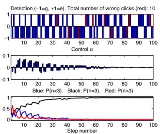
Any real experimental setup includes imperfection and error. To test the robustness of the feedback scheme, a false

detection probability ηf =101 is introduced. In case of false

detection at step k, the atom is detected in g (resp. e) whereas it collapses effectively in e (resp. g). This means that in (15),

sk = g (resp. sk = e), whereas in (2), it is the converse

Mk = Me (resp. Mk = Mg). Simulations of figure 3 differ

from those of figure 2 by only ηf = 101: we observe for

this sample trajectory a longer convergence time. A much

more significative impact of ηfis given by ensemble average.

Figure 4 presents ensemble averages corresponding to the

third sub-plot of figures 2 and 3. For ηf = 0 (left plot), we

observe an average fidelity Tr (ρkρ) converging to 100%:¯

it exceeds 90% after k = 40 steps. For ηf = 1/10, the

asymptotic fidelity remains under 80% and reaches 70% after 30 iteration. The performance are reduced but not changed dramatically. The proposed feedback scheme appears to be robust to such experimental errors.

10 20 30 40 50 60 70 80 90 100 −1

0 1

Detection (−1=g, +1=e). Total number of wrong clicks (red): 0

10 20 30 40 50 60 70 80 90 100 −0.1 0 0.1 Control α 10 20 30 40 50 60 70 80 90 100 0 0.5 1

Blue: P(n<3). Black: P(n=3). Red: P(n>3)

Step number

Fig. 2. A single closed-loop quantum trajectory in the ideal case (¯n = 3).

10 20 30 40 50 60 70 80 90 100 −1

0 1

Detection (−1=g, +1=e). Total number of wrong clicks (red): 10

10 20 30 40 50 60 70 80 90 100 −0.1 0 0.1 Control α 10 20 30 40 50 60 70 80 90 100 0 0.5 1

Blue: P(n<3). Black: P(n=3). Red: P(n>3)

Step number

Fig. 3. A single closed-loop quantum trajectory with a false detection probability of 1/10. 10 20 30 40 50 60 70 80 90 100 0 0.1 0.2 0.3 0.4 0.5 0.6 0.7 0.8 0.9 1 proba.

Blue: P(n<3). Black: P(n=3). Red: P(n>3)

Step number 10 20 30 40 50 60 70 80 90 100 0 0.1 0.2 0.3 0.4 0.5 0.6 0.7 0.8 0.9 1 proba.

Blue: P(n<3). Black: P(n=3). Red: P(n>3)

Step number

Fig. 4. Averages of 104 _{closed-loop quantum trajectories similar to the}

one of figure 2 (left, ηf = 0) and 3 (right, ηf= ₁₀1).

VI. CONCLUSION

In [2] more realistic simulations are reported. They include nonlinear shift per photon (N φ replaced by a non linear function Φ(N ) in (1)) and additional experimental errors such as detector efficiency and delays. These simulations confirm the robustness of the feedback scheme, robustness that needs to be understood in a more theoretical way. In particular, it seems that the quantum filter (15) forgets its

initial condition ρest

0 almost surely and thus admits some

strong contraction properties as indicated by Theorem 3.

With the truncation to nmax_{photons, convergence is proved}

only in the finite dimensional case. But feedback (7) and

quantum filter (15) are still valid for nmax

= +∞. We conjecture that Theorems 1 and 2 remain valid in this case. In the experimental results reported in [10], [5], [4] the time-interval corresponding to a sampling step is around 100µs. Thus it is possible to implement, on a digital com-puter and in real-time, the Lyapunov feedback-law (7) where ρ is given by the quantum filter (15).

VII. APPENDIX:STABILITY THEORY FOR STOCHASTIC

PROCESSES

We recall here Doob’s inequality and Kushner’s invariance theorem. For detailed discussions and proofs we refer to [8] (Sections 8.4 and 8.5).

Theorem 4 (Doob’s Inequality): Let {Xn} be a Markov

chain on state space S. Suppose that there is a non-negative

function V (x) satisfying

_E

(V (X1) | X0= x) − V (x) =

−k(x), where k(x) ≥ 0 on the set {s : V (x) < λ} ≡ Qλ.

Then

_P

) sup ∞>n≥0 V (Xn) ≥ λ | X0= x * ≤ V(x)λ .

Further-more, there is some random v ≥ 0, so that for paths never

leaving Qλ, V (Xn) → v ≥ 0 almost surely.

For the statement of the second Theorem, we need to use the language of probability measures rather than the random process. Therefore, we deal with the space M of probability

measures on the state space S. Let µ0 = ϕ be the initial

probability distribution (everywhere through this paper we

have dealt with the case where µ0is a dirac on a state ρ0 of

the state space of density matrices). Then, the probability

distribution of Xn, given initial distribution ϕ, is to be

denoted by µn(ϕ). Note that for m ≥ 0, the Markov property

implies: µn+m(ϕ) = µn(µm(ϕ)).

Theorem 5 (Kushner’s invariance Theorem): Consider

the same assumptions as that of the Theorem 4. Let µ0= ϕ

be concentrated on a state x0∈ Qλ (Qλ being defined as in

Theorem 4), i.e. ϕ(x0) = 1. Assume that 0 ≤ k(Xn) → 0

in Qλ implies that Xn → {x | k(x) = 0} ∩ Qλ ≡ Kλ.

Under the conditions of Theorem 4, for trajectories never

leaving Qλ, Xn converges to Kλ almost surely. Also, the

associated conditioned probability measures ˜µn tend to the

largest invariant set of measures M whose support set is

in Kλ. Finally, for the trajectories never leaving Qλ, Xn

REFERENCES

[1] M. Brune, S. Haroche, J.-M. Raimond, L. Davidovich, and N. Za-gury. Manipulation of photons in a cavity by dispersive atom-field coupling: Quantum-nondemolition measurements and g´en´eration of ”Schr¨odinger cat” states. Physical Review A, 45(7):5193–5214, 1992. [2] I. Dotsenko, M. Mirrahimi, M. Brune, S. Haroche, J.-M. Raimond, and P. Rouchon. Quantum feedback by discrete quantum non-demolition measurements: towards on-demand generation of photon-number states. http://arxiv.org/abs/0905.0114, 2009. submitted. [3] J.M. Geremia. Deterministic and nondestructively verifiable

prepara-tion of photon number states. Physical Review Letters, 97(073601), 2006.

[4] S. Gleyzes, S. Kuhr, C. Guerlin, J. Bernu, S. Del´eglise, U. Busk Hoff, M. Brune, J.-M. Raimond, and S. Haroche. Quantum jumps of light recording the birth and death of a photon in a cavity. Nature, 446:297– 300, 2007.

[5] C. Guerlin, J. Bernu, S. Del´eglise, C. Sayrin, S. Gleyzes, S. Kuhr, M. Brune, J.-M. Raimond, and S. Haroche. Progressive field-state collapse and quantum non-demolition photon counting. Nature,

448:889–893, 2007.

[6] S. Haroche and J.M. Raimond. Exploring the Quantum: Atoms, Cavities and Photons. Oxford University Press, 2006.

[7] T. Kailath. Linear Systems. Prentice-Hall, Englewood Cliffs, NJ, 1980. [8] H.J. Kushner. Introduction to stochastic control. Holt, Rinehart and

Wilson, INC., 1971.

[9] M. Mirrahimi and R. Van Handel. Stabilizing feedback controls for quantum systems. SIAM Journal on Control and Optimization, 46(2):445–467, 2007.

[10] Del´eglise S., I. Dotsenko, C. Sayrin, J. Bernu, M. Brune, J.-M. Raimond, and S. Haroche. Reconstruction of non-classical cavity field states with snapshots of their decoherence. Nature, 455:510– 514, 2008.

[11] S. G. Schirmer, H. Fu, and A. I. Solomon. Complete controllability of quantum systems. Phys. Rev. A, 63(063410), 2001.