HAL Id: hal-01632805
https://hal-mines-paristech.archives-ouvertes.fr/hal-01632805
Submitted on 10 Nov 2017
HAL is a multi-disciplinary open access archive for the deposit and dissemination of sci-entific research documents, whether they are pub-lished or not. The documents may come from teaching and research institutions in France or abroad, or from public or private research centers.
L’archive ouverte pluridisciplinaire HAL, est destinée au dépôt et à la diffusion de documents scientifiques de niveau recherche, publiés ou non, émanant des établissements d’enseignement et de recherche français ou étrangers, des laboratoires publics ou privés.
New experimental density data and derived
thermophysical properties of carbon dioxide – Sulphur
dioxide binary mixture (CO 2 -SO 2 ) in gas, liquid and
supercritical phases from 273 K to 353 K and at
pressures up to 42 MPa
Mahmoud Nazeri, Antonin Chapoy, Alain Valtz, Christophe Coquelet,
Bahman Tohidi
To cite this version:
Mahmoud Nazeri, Antonin Chapoy, Alain Valtz, Christophe Coquelet, Bahman Tohidi. New experi-mental density data and derived thermophysical properties of carbon dioxide – Sulphur dioxide binary mixture (CO 2 -SO 2 ) in gas, liquid and supercritical phases from 273 K to 353 K and at pressures up to 42 MPa. Fluid Phase Equilibria, Elsevier, 2017, 454, pp.64-77. �10.1016/j.fluid.2017.09.014�. �hal-01632805�
1
New experimental density data and derived thermophysical properties of
carbon dioxide – Sulphur dioxide binary mixture (CO2 - SO2) in gas, liquid
and supercritical phases from 273 K to 353 K and at pressures up to 42
MPa
Mahmoud Nazeria*, Antonin Chapoya,b*, Alain Valtzb, Christophe Coqueletb, Bahman Tohidia
a
Hydrates, Flow Assurance & Phase Equilibria Research Group, Institute of Petroleum Engineering, Heriot-Watt University, Edinburgh, EH14 4AS, UK
b
MINES ParisTech PSL Research University, CTP-Centre of Thermodynamics of Processes, 35, Rue Saint Honoré, 77305 Fontainebleau, France
* Corresponding Authors: Mahmoud Nazeri (M.Nazeri@hw.ac.uk) Antonin Chapoy (A.Chapoy@hw.ac.uk)
ABSTRACT
Due in part to the toxicity of the CO2-SO2 binary system, there are no density data available
in the literature. Densities for this system were measured using a vibrating tube densitometer (VTD), Anton Paar DMA 512, and the forced path mechanical calibration (FPMC) method in the gas, liquid and supercritical phases at pressures up to 41.7 MPa. The mole fraction of the mixture was 0.9478 CO2 + 0.0522 SO2 at 298 K and 0.9503 CO2 + 0.0497 SO2 at 273, 283,
323 and 353 K. The compressibility factor, isobaric heat capacity and bubble points were also derived from the measured densities. The classical cubic equations of state, i.e., Soave-Redlich-Kwong (SRK), Peng-Robinson (PR) and Valderrama version of Patel-Teja (VPT) with the CO2 volume correction term and Peneloux shift parameter in addition to a multi
parameter EoS based on Helmholtz energy were evaluated using the measured density data. The most accurate EoSs for the investigated system were the multi parameter EoS and the PR-CO2 with overall AAD of 0.6% and 1.0%, respectively.
Keywords: Density, Carbon capture transport and storage (CCS), CO2, Sulphur Dioxide
2 1. Introduction
High demand for energy due to the rapid economic growth resulted in an ever increasing use of fossil fuels, i.e. coal, oil and natural gas following the industrial revolution. The effect of this has been to increase the amount of greenhouse gases such as CO2 in the atmosphere.
Carbon capture and storage (CCS) is the name given to technology based solutions aimed at reducing CO2 emissions to the atmosphere [1]. This technology comprises capturing CO2
during burning of fossil fuels, compression and transport mainly via pipelines and injection into geological storage basins. The captured CO2 will contain ranges of impurities depend on
the source of fossil fuel as well as the capturing technology [2][3].
Sulphur dioxide can be present in heavy oil production or in flue gas in the post-combustion or oxyfuel processes in coal-fired power plants. In the MEA-based absorption processes, impurities such as O2, NO2 and SO2 can lead to severe operational problems such as foaming,
viscosity increase and formation of heat-stable salts. The typical range of SO2 in the
MEA-based post-combustion processes is 500-3000 part per million by volume (ppmv). Flue gas
desulphurisation (FGD) units with wet SO2 scrubbers can absorb 80-95% of the SO2 in the
flue gas before entering the CO2 absorber. However, in case of failure in the FGD unit, 75%
of the SO2 could be absorbed by MEA as it is not selective a solvent to acid gases [2]. The
presence of SO2 can make problems such as corrosion in the presence of water [4] in the
transportation of captured CO2 with impurities from both MEA-based post-combustion or
oxyfuel processes [5][6].
Due to the toxicity of SO2, the Immediately Dangerous to Life and Health (IDLH)
concentration of this component is set to 100 ppmv by the National Institute for Occupational
Safety and Health (NIOSH) [7]. Shell Cansolv also commissioned an integrated system to capture CO2 and SO2 simultaneously in a commercial scale post-combustion coal fired power
plant in Saskatchewan. The captured CO2 is transported for the CO2 Enhanced Oil Recovery
(CO2-EOR) in Weyburn oil field and SO2 is used to produce sulphuric acid as a valuable
by-product [8].
Similar to injection of acid gases, i.e., injection of CO2 - H2S [9][10], technically, CO2 and
SO2 can be co-stored in deep saline aquifers and this effectively reduces the capture cost by
avoiding SO2 removal costs [11][12][13]. However, the reactivity of SO2 with rock in the
3
effects can reduce the pH of the formation water, change the porosity of reservoir rock and cause mineral dissolution and sulphate precipitation [11][17][18][19][20].
A proper understanding of the thermodynamic and transport properties of CO2-SO2 systems
is required as an input to feasibility studies and equipment sizing in the above processes [21]. The presence of impurities in the captured streams of CO2 would affect the thermophysical
properties, in particular density and viscosity, of high CO2 content mixtures. Equations of
state (EoSs) should be evaluated using the experimental density and vapour-liquid equilibrium (VLE) data. The lack of experimental data for CO2-SO2 systems is certainly due
to toxicity of the system [22]. The only available data for this system is reported by Caubet
[23] in 1904. A comprehensive thermodynamic behaviour of CO2-SO2 mixture was studied
experimentally by Coquelet and co-workers [24], [25] for transport purposes of CO2 mixtures
in a CCS context. Only VLE data are available at 263.15 K and 333.21 K and at pressures ranging from 0.1 to 8.8 MPa.
In this work, the densities of approximately 95 mol% CO2 with 5 mol% SO2 were measured
using a Vibrating Tube Densitometer (VTD) in the gas, liquid and supercritical phases. The measurements were carried out at five isotherms 273, 283, 298, 323 and 353 K at pressures up to 42 MPa. Thermodynamic properties such as compressibility factor, isobaric specific heat capacity and bubble points were obtained from the measured densities. The measured densities also were employed to evaluate the classical cubic EoSs, i.e., Soave-Redlich-Kwong (SRK-EoS) [26], Peng-Robinson (PR-ES) [27], and Valderrama modification of the [28]
Patel-Teja (VPT-EoS) [29] EoSs. Then, to improve the density prediction, the CO2 volume
correction term [30] and Peneloux shift parameter [31] were introduced to those EoSs. Also, a multi parameter EoS based on Helmholtz energy [32][33] with the short industrial equation from Lemmon & Span for pure SO2[34] (see Appendix A) and Span &Wagner EoS for pure
CO2 [35] was evaluated using the measured density data and derived thermodynamic
properties.
2. Experimental part
Experimental work was carried out in the high safety laboratory at CTP - Centre of Thermodynamics of Processes research group at Mines ParisTech in France.
4 2.1. Material
A binary mixture of CO2-SO2 was prepared to perform density measurements. Table 1 shows
the details of the chemicals, suppliers and purities of the components used in this study. A pressure vessel with a volume of 100 mL was vacuumed and then after disconnecting from the vacuum pump, the mass was measured using a balance with four digit after the decimal point (brand: Sartorius) three times. Due to the lower vapour pressure of SO2 (0.35 MPa at
293 K) compared to CO2 (with a vapour pressure of 5.73 MPa at 293 K), first SO2 was
injected to the vacuumed pressure vessel. After neutralising the SO2 trapped in the line using
sodium hydroxide (NaOH) considering acid base reaction, the pressure vessel was disconnected and the weight was measured to obtain the exact amount of injected SO2. The
weight of injected SO2 was 6.357 g. The pressure vessel then was connected to the CO2
cylinder in order to inject CO2. After disconnecting the pressure vessel and weighing with the
balance, the amount of injected CO2 was 79.229 g. After calculations, the mole percent for
SO2 and CO2 was 5.22 mol% with ur(z) = 0.010 mol% 94.78 mol% with ur(z) = 0.180 mol%, respectively. The uncertainties are reported with 95% confidence level (coverage factor k=2). The prepared binary mixture was then used to perform density measurements at 298 K. Due to a leak through the piston to the nitrogen side resulting in a change in the composition, another binary mixture was prepared with a similar procedure to conduct the density measurements at the other isotherms. The amount of injected SO2 and CO2 was 4.579 and
60.183 g, respectively. The mole percent and uncertainties with 95% confidence level were 4.97 mol% with ur(z) = 0.010 mol% for SO2 and 95.03 mol% with ur(z) = 0.181 mol% for
CO2, respectively.
2.2. Equipment description
A Vibrating Tube Densitometer (VTD), Anton Paar DMA 512 was used to measure the densities. Figure 1 shows a schematic view of the setup which has been thoroughly described in previous publication [36][37]. Briefly, the main part of the setup is a U-shaped vibrating tube Anton Paar densitometer (1) with a working pressure of up to 70 MPa and temperature range of 263 – 423 K. The tube material is Hastelloy. A jacket through which fluid is circulated from a liquid bath (4) surrounds the densitometer allowing control of the temperature with a stability of ±0.02 K. The sample fluid flows from the 150 ml, 70 MPa rated pressurised vessel (2) to the densitometer through a tube with a diameter of 1.6 mm
5
(1/16 inches) and pressure rating of 100 MPa. The connecting tubes are fully immersed in a temperature controlled liquid bath model West P6100 (5).
The pressure of setup is measured with three pressure transducers (model: Druck PTX611) (6) with ranges of 0-10 MPa, 10-30 MPa and 30-70 MPa. The transducers were calibrated with an electronic balance (model: GE Sensing PACE 5000) at pressure up to 20 MPa and using a dead weight tester (model: Desgranges & Huot 5202S) for pressures from 20 to 40 MPa. The pressure transducers can measure the pressure with standard uncertainties of u(p) = 0.002 MPa , u(p) = 0.005 MPa and u(p) = 0.005 MPa in the ranges of 0-10 MPa, 10-30 MPa and 30-70 MPa, respectively. The temperature of the densitometer and the liquid bath were measured using four-wire 100-Ω platinum resistance probes (Pt100) (7). The probes were calibrated against a reference thermometer with 25-Ω (model: Tinsley Precision Instrument). The standard uncertainty of the temperature probes were estimated to be u(T) = 0.02 K after calibration. The pressure and temperature were recorded using an Agilent HP34970A data acquisition unit (10). The vibration period, τ, also was recorded using a HP53131A data acquisition unit (10).
2.3. Calibration and measurement procedures
The densitometer was firstly calibrated using pure CO2 as a reference fluid and forced path
mechanical calibration (FPMC) model developed by Bouchot and Richon [38][39][40]. This method considers that the vibrating tube is represented by a box with a known internal volume, V, and a known mass of tube M0. The box is connected to a support with a spring with a constant of stiffness, K. Consequently, the period of vibration, τ, is expressed by: , with . In this model, the stress and strain behaviour of the tube
material would be represented from the realistic mechanical considerations. The reference fluid is used to set the magnitude of pressure independent from temperature. The following equation shows the frame for the FPMC model:
(1)
Where ρ is the density of inner fluid, M0 is the mass of the tube under vacuum, Vi is the internal volume, K is the natural transversal stiffness and τ is the vibrating period. The subscript 0 indicates the vacuum condition. By considering the tube as a thick-walled cylinder and replacing terms for the M0/Vi and K/K0, the complete FPMC model can be formulated as [38]:
6 (2) The density data obtained from the Span and Wagner EoS [41] were used as a reference densities to tune the unknown parameters, (M0/L00) and γT, in this model at the full range of
pressures for each measured isotherm. The measurement procedure as well as the method to determine the combined standard uncertainties [42][43] for each measured density were well described in the authors’ previous publication [36].
3. Specific heat capacity calculations
The residual specific heat capacity ( ) can be calculated from the measured density data through the following equation [44]:
(3)
In this equation, the gradient of molar volume with temperature at each constant pressure were plotted using the measured densities at the five measured isotherms. The procedure to calculate the specific heat capacity from Equation (3) has also been described in a previous publication for the CO2-H2S system [36]. A similar procedure was undertaken in this work.
The constants B to F in the Aly & Lee equation [45] to calculate the ideal gas specific heat capacity, C0pi, for CO2 and SO2 components is summarised in Table 2. The obtained
0 pi
C from the Aly & Lee equation [45] is in J.K-1.kmol-1.
4. Results and discussions
Densities of CO2-SO2 binary systems were measured using vibrating tube densitometer
(VTD), Anton Paar DMA 512 in the gas, liquid and supercritical phases at pressures up to 41.7 MPa. The composition of the binary system was 0.9478 CO2 + 0.0522 SO2 at 298 K and
0.9503 CO2 + 0.0497 SO2 at 273, 283, 323 and 353 K. At each isotherm, the densitometer
was firstly calibrated using pure CO2 with a forced path mechanical calibration (FPMC)
technique [38]. The measured densities along with their uncertainties and compressibility factor at each corresponding pressure, temperature and phase are reported in Tables 3 through
7 for each isotherm. The uncertainty values in the gas, liquid and supercritical phases are summarised for each isotherm in Table 8. The measured densities then are compared against various equations of state including Soave-Redlich-Kwong [26] (SRK), Peng-Robinson [27]
7
volume fraction [30][46] and Peneloux shift parameter [31] as well as multi parameter equation of state based on Helmholtz energy [33]. In this work, the modified binary interaction parameter, kij or BIP, for the CO2-SO2 was 0.02 for all cubic EoSs. The Average
Absolute Deviation (AAD) of these model predictions from the obtained density data was calculated from the following equation:
(4)
Table 9 summarises the AAD and Maximum Absolute Deviation (MAD) of the investigated
EoSs in the gas, liquid and supercritical phases as well as the overall quantities. Thermodynamic properties of the investigated mixtures, i.e., compressibility factor, isobaric specific heat capacity and bubble points, were derived from the measured densities. Table 10
gives the derived specific heat capacities of the binary system and predicted quantities with the multi parameter EoS. The bubble points of the mixture are summarised at two isotherms in Table 11.
The measured densities, as shown in Table 3 to 7, varies over a wide range from 1.0 kg/m3 at 297.42 k and 0.051 MPa to 1110.7 kg/m3 at 273.54 K and 41.723 MPa. Overall (see Table 8), 454 density data were obtained of which 97 points were in the gas phase, 221 points in the liquid phase and 136 points in the supercritical phase. Figure 2 demonstrates the measured and predicted densities using multi parameter EoS at different isotherms. Values at lower pressures, i.e. pressures less than 8 MPa and densities below 200 kg/m3 are shown in Figure 3.
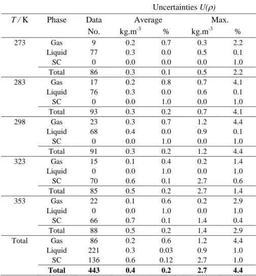
The maximum uncertainty of the measured densities [42][43], as shown in Table 8, is ur(ρ) = 4.4% in the gas phase at 298 K and very low pressure conditions. However, the average uncertainty in the gas phase at all isotherms is ur(ρ) = 0.6%. The average uncertainty in the liquid phase is also ur(ρ) = 0.03% with the maximum value of ur(ρ) = 1.0%. Those in the supercritical phase is ur(ρ) = 0.1% and ur(ρ) = 1.0% for the average and maximum uncertainties, respectively. Overall, the average uncertainty for the measured densities is u(ρ) = 0.4 kg/m3 or ur(ρ) = 0.2% with the maximum value of u(ρ) = 2.7 kg/m3 or ur(ρ) = 4.4%.
The measured densities using VTD densitometer with the FPMC calibration procedure in this work, were already validated in the authors’ previous publication [36] for the CO2-H2S
8
system by comparing the measured values of CO2-H2S to the data published by Stouffer et al.
[47][48] at two isotherms.
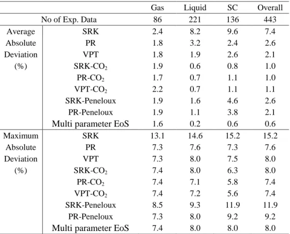
The measured densities were employed to evaluate accuracy of various equations of state in this work. As summarised in Table 9, first the classical cubic EoSs were tested. The AAD for the SRK-EoS in the gas, liquid and supercritical phases is 2.4%, 8.2% and 9.6% with an overall AAD of 7.4% and MAD of 15.2%. Those for the PR-EoS was 1.8%, 3.2% and 2.4% with an overall AAD of 2.6% and MAD of 7.6%. The AAD for the VPT-EoS is 1.8%, 1.9% and 2.6% in the gas, liquid and supercritical phases with an overall AAD of 2.1%. The most accurate EoS in the gas phase is VPT and PR EoSs with an AAD of 1.8%, VPT-EoS in the liquid phase with the AAD of 1.9% and PR-EoS in the supercritical phase with the AAD of 2.4%. However, the VPT-EoS is the most accurate among them with the overall AAD of 2.1% and MAD of 8.0%.
Introducing the CO2 correction term [30][46] to the above EoSs then could significantly
improve their prediction accuracy for the densities of the investigated binary system. The overall AAD of SRK-CO2 and PR-CO2 EoSs is 1.0% (reduced from 7.4% and 2.6% to 1.0%)
which are the most accurate EoSs with the CO2 volume correction term. The MAD for these
are 8.0 and 7.4%, respectively. PR-CO2 in the gas phase (with the AAD of 1.7%) and
SRK-CO2 in the liquid and supercritical phases (with the AAD of 0.6% and 0.8%) are the most
accurate EoS in the different phases. In addition to the CO2 volume correction term, the
Peneloux shift parameter also was introduced to the SRK and PR EoSs. This could also reduce the overall AAD to 2.6% and 2.1% for the SRK and PR EoSs, respectively. Among all classical cubic EoSs, the PR-CO2 with the AAD and MAD of 1.0% and 7.4% is the most
accurate EoS for the investigated mixture.
Apart from classical cubic EoSs, the multi parameter EoS also were evaluated using the measured densities. As shown in Table 9, the multi parameter EoS predicts the densities more accurately compared to the classical EoSs. The AAD of multi parameter EoS from the measured densities in the gas, liquid and supercritical phases are 1.6%, 0.2% and 0.6% with the overall AAD and MAD of 0.6% and 8.0%. Figure 4 shows the deviations of the multi parameter EoS from the measured densities.
The compressibility factor of the investigated mixture were derived from the measured densities, which were reported in Tables 3 to 7. Figures 5 and 6 show the derived z-factors at
9
all pressure ranges and at pressures lower than 10 MPa, respectively. The lines in these figures demonstrate the predicted z-factors using the multi parameter EoS at each isotherms. As can be seen, they are in good agreement and the AAD of the multi parameter EoS from the derived z-factors is 1.6%, 0.2% and 0.6% in the gas, liquid and supercritical phases. The overall AAD is also 0.6%.
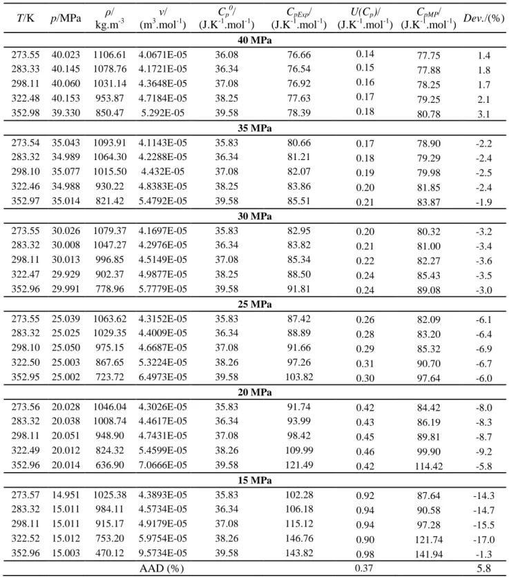
The isobaric specific heat capacities were calculated from thermodynamic equations and using the measured densities at various pressure and temperature. The Cp were calculated at the constant pressures of 15, 20, 25, 30, 35 and 40 MPa using Equation (3). The measured specific heat capacities were compared against the predictions using the multi parameter EoS. As shown in Table 10, the AAD of the multi parameter EoS from the derived values is 5.8% which shows the model predictions and the experimentally derived values are in the good agreement. Figure 7 also shows the determined specific heat capacities at different pressures. The lines in the figure show the predicted specific heat capacities using the multi parameter EoS. However, it is suggested that these values should be compared to the directly measured heat capacities, e.g., measured Cp using adapted calorimeters.
The procedure of conducting the tests in each isotherm was injecting the sample fluid at a very slow rate to reach the dew point and continuing on the injection to reach the bubble point and further injection to achieve the desired pressure. Continuous data recording during the test, particularly in the vicinity of the dew and bubble points, allows fitting the representative correlation to the experimental data on each side of the dew or bubble point. Therefore, the precise location of the dew or bubble point could be determined by crossing the fitted correlations. The calculated bubble points at two isotherms of 273 K and 283 K as well as the predicted amounts using PR-CO2 EoS were summarised in Table 11. An overall
AAD of 3.6% was achieved by comparing the measured and predicted values. Figures 8
shows the bubble point measurements. The circle points in this figure show the cross points of the fitted correlations which correspond to the dew or bubble points. The conclusion of this comparison is that the densitometer is not very accurate for estimation of bubble and dew point pressure. In comparison with VLE prediction using PR-CO2 EoS, there is a difference
of at least 0.1MPa, which is higher than experimental uncertainty of pressure using the static analytical method [25].
10 5. Conclusion
The densities of CO2-SO2 binary mixture were measured using VTD densitometer, Anton
Paar DMA 512, in the gas, liquid and supercritical phases. The densitometer was first calibrated using pure CO2 and the FPMC calibration technique. Then, the densities of a
0.9503 CO2 – 0.0497 SO2 mixture were measured at temperatures of 273, 283, 323 and 353
K. In addition the densities of 0.9478 CO2 – 0.0522 SO2 were measured at 298 K. The overall
average uncertainty of the measured densities with a confidence level of 95% was ur(ρ) = 0.2% or u(ρ) = 0.4 kg/m3. The highest uncertainties were observed at very low pressure conditions in the gas phase or in the vicinity of the bubble point curve in the liquid phase. The measured densities were employed to evaluate classical cubic EoSs, those with CO2
volume correction term and Peneloux shift parameter as well as the multi parameter EoS. Among the classical EoSs, the PR-CO2 was the most accurate EoS for the investigated
mixture with an AAD of 1.0% and MAD of 7.4%. However, the multi parameter EoS was the most accurate EoS with an AAD of only 0.6% and MAD of 8.0%. From the measured densities for the CO2-SO2 system, the thermodynamic properties were derived and compared
to the EoSs. The compressibility factor was in a good agreement with the multi parameter EoS with an AAD of 0.6%. The isobaric specific heat capacity was derived from thermodynamic equations and measured densities. The AAD of the predicted specific heat capacity using the multi parameter EoS from the derived quantities was 5.8%. The bubble points at two different isotherms of 273 and 283 K were measured by fitting the equations to the numerous measured densities on both sides of bubble points. The AAD of the predicted bubble points using PR-CO2 EoS from the measured values was 3.6%.
11 6. Acknowledgements
This work was a part of the JIP project” Impact of Common Impurities on Carbon Dioxide Capture, Transport and Storage” [30] which the phase-I was conducted jointly at Heriot-Watt University in Edinburgh, UK and MINES ParisTech in France in 2011-2014. The authors would like to gratefully acknowledge the sponsors of the project: Chevron, GALP Energia, Linde AG Engineering Division, OMV, Petroleum Expert, Statoil, TOTAL and National Grid Carbon Ltd. The thermophysical properties of CO2-rich fluids where investigated during the
course of project are phase equilibira, hydrates [49], solid formation, density [36][46][50], viscosity, interfacial tension [51], solubility [52][53][54] and pH.
12 REFERENCES
[1] D. Y. C. Leung, G. Caramanna, and M. M. Maroto-Valer, “An overview of current status of carbon dioxide capture and storage technologies,” Renew. Sustain. Energy
Rev., vol. 39, pp. 426–443, 2014.
[2] J.-Y. Lee, T. C. Keener, and Y. J. Yang, “Potential Flue Gas Impurities in Carbon Dioxide Streams Separated from Coal-Fired Power Plants,” J. Air Waste Manage.
Assoc., vol. 59, no. 6, pp. 725–732, Feb. 2012.
[3] R. T. J. Porter, M. Fairweather, M. Pourkashanian, and R. M. Woolley, “The range and level of impurities in CO2 streams from different carbon capture sources,” Int. J.
Greenh. Gas Control, vol. 36, pp. 161–174, May 2015.
[4] F. Farelas, Y. S. Choi, and S. Nešić, “Corrosion Behavior of API 5L X65 Carbon Steel Under Supercritical and Liquid Carbon Dioxide Phases in the Presence of Water and Sulfur Dioxide,” Corrosion, vol. 69, no. 3, pp. 243–250, Mar. 2013.
[5] D. Liu, T. Wall, and R. Stanger, “CO2 quality control in Oxy-fuel technology for CCS: SO2 removal by the caustic scrubber in Callide Oxy-fuel Project,” Int. J. Greenh. Gas
Control, vol. 51, pp. 207–217, 2016.
[6] A. Kather and S. Kownatzki, “Assessment of the different parameters affecting the CO2 purity from coal fired oxyfuel process,” Int. J. Greenh. Gas Control, vol. 5, pp. S204–S209, Jun. 2011.
[7] M. Woods and M. Matuszewski, “Quality Guideline for Energy System Studies: CO2 Impurity Design Parameters, NETL/DOE-341/011212, 2013.”
[8] K. Stéphenne, “Start-up of World’s First Commercial Post-combustion Coal Fired CCS Project: Contribution of Shell Cansolv to SaskPower Boundary Dam ICCS Project,” Energy Procedia, vol. 63, pp. 6106–6110, 2014.
[9] S. Bachu and W. D. Gunter, “Overview of acid-gas injection operations in western Canada,” Proc. 7th Int. Conf. Greenh. Gas Control Technol. vol. 1. Peer-Reviewed
Pap. Plenary Present. IEA Greenh. Gas R&D Program. Cheltenham, UK, 2005.
[10] A. Battistelli, P. Ceragioli, and M. Marcolini, “Injection of Acid Gas Mixtures in Sour Oil Reservoirs: Analysis of Near-Wellbore Processes with Coupled Modelling of Well and Reservoir Flow,” Transp. Porous Media, vol. 90, no. 1, pp. 233–251, Nov. 2010. [11] Z. Wang, J. Wang, C. Lan, I. He, V. Ko, D. Ryan, and A. Wigston, “A study on the
impact of SO2 on CO2 injectivity for CO2 storage in a Canadian saline aquifer,” Appl.
Energy, vol. 184, pp. 329–336, 2016.
[12] Q. Li, X. Li, N. Wei, and Z. Fang, “Possibilities and potentials of geological co-storage CO2 and SO2 in China,” Energy Procedia, vol. 4, pp. 6015–6020, 2011.
[13] R. Miri, P. Aagaard, and H. Hellevang, “Examination of CO2 - SO2 Solubility in Water by SAFT1. Implications for CO2 Transport and Storage,” J. Phys. Chem. B, vol. 118, no. 34, pp. 10214–10223, Aug. 2014.
[14] J. Zhu and D. Harris, “Modeling potential impacts of SO2 co-injected with CO2 on the Knox Group, western Kentucky | American Geosciences Institute,” 2016.
[15] Z. Ziabakhsh-Ganji and H. Kooi, “Sensitivity of the CO2 storage capacity of underground geological structures to the presence of SO2 and other impurities,” Appl.
13
[16] J. K. Pearce, G. K. W. Dawson, A. C. K. Law, D. Biddle, and S. D. Golding, “Reactivity of micas and cap-rock in wet supercritical CO2 with SO2 and O2 at CO2 storage conditions,” Appl. Geochemistry, vol. 72, pp. 59–76, 2016.
[17] S. García, Q. Liu, and M. M. Maroto-Valer, “A novel high pressure-high temperature experimental apparatus to study sequestration of CO2 - SO2 mixtures in geological formations,” Greenh. Gases Sci. Technol., vol. 4, no. 4, pp. 544–554, Aug. 2014. [18] IEAGHG, “Effects of Impurities on Geological Storage of CO2, Report 2011/04,”
2011.
[19] S. P. Tan, Y. Yao, and M. Piri, “Modeling the Solubility of SO2 + CO2 Mixtures in Brine at Elevated Pressures and Temperatures,” Ind. Eng. Chem. Res., vol. 52, no. 31, pp. 10864–10872, Aug. 2013.
[20] S. Waldmann and H. Rütters, “Geochemical effects of SO2 during CO2 storage in deep saline reservoir sandstones of Permian age (Rotliegend) – A modeling approach,”
Int. J. Greenh. Gas Control, vol. 46, pp. 116–135, 2016.
[21] E. Hendriks, G. M. Kontogeorgis, R. Dohrn, J.-C. de Hemptinne, I. G. Economou, L. F. ilnik, and V. Vesovic, “Industrial Requirements for Thermodynamics and Transport Properties,” Ind. Eng. Chem. Res., vol. 49, no. 22, pp. 11131–11141, Nov. 2010.
[22] H. Li, J. P. Jakobsen, Ø. Wilhelmsen, and J. Yan, “PVTxy properties of CO2 mixtures relevant for CO2 capture, transport and storage: Review of available experimental data and theoretical models,” Appl. Energy, vol. 88, no. 11, pp. 3567–3579, Nov. 2011. [23] M. F. Caubet, “Liquéfaction des mélanges gazeux. Université de Bordeaux Thesis.”
1901.
[24] V. Lachet, T. de Bruin, P. Ungerer, C. Coquelet, A. Valtz, V. Hasanov, F. Lockwood, and D. Richon, “Thermodynamic behavior of the CO2+SO2 mixture: Experimental and Monte Carlo simulation studies,” Energy Procedia, vol. 1, no. 1, pp. 1641–1647, Feb. 2009.
[25] C. Coquelet, A. Valtz, and P. Arpentinier, “Thermodynamic study of binary and ternary systems containing CO2+impurities in the context of CO2 transportation,”
Fluid Phase Equilib., vol. 382, pp. 205–211, Nov. 2014.
[26] G. Soave, “Equilibrium constants from a modified Redlich-Kwong equation of state,”
Chem. Eng. Sci., vol. 27, no. 6, pp. 1197–1203, Jun. 1972.
[27] D.-Y. Peng and D. B. Robinson, “A New Two-Constant Equation of State,” Ind. Eng.
Chem. Fundam., vol. 15, no. 1, pp. 59–64, Feb. 1976.
[28] J. O. Valderrama, “A generalized Patel-Teja equation of state for polar and nonpolar fluids and their mixtures.,” J. Chem. Eng. JAPAN, vol. 23, no. 1, pp. 87–91, Mar. 1990.
[29] N. C. Patel and A. S. Teja, “A new cubic equation of state for fluids and fluid mixtures,” Chem. Eng. Sci., vol. 37, no. 3, pp. 463–473, 1982.
[30] A. Chapoy, M. Nazeri, M. Kapateh, R. Burgass, C. Coquelet, and B. Tohidi, “Effect of impurities on thermophysical properties and phase behaviour of a CO2-rich system in CCS,” Int. J. Greenh. Gas Control, vol. 19, pp. 92–100, Nov. 2013.
[31] A. Péneloux, E. Rauzy, and R. Fréze, “A consistent correction for Redlich-Kwong-Soave volumes,” Fluid Phase Equilib., vol. 8, no. 1, pp. 7–23, Jan. 1982.
14
[32] O. Kunz and W. Wagner, “The GERG-2008 Wide-Range Equation of State for Natural Gases and Other Mixtures: An Expansion of GERG-2004,” J. Chem. Eng. Data, vol. 57, no. 11, pp. 3032–3091, Nov. 2012.
[33] J. Gernert and R. Span, “EOS–CG: A Helmholtz energy mixture model for humid gases and CCS mixtures,” J. Chem. Thermodyn., vol. 93, pp. 274–293, 2016.
[34] E. W. Lemmon and R. Span, “Short Fundamental Equations of State for 20 Industrial Fluids,” 2006.
[35] R. Span and W. Wagner, “A New Equation of State for Carbon Dioxide Covering the Fluid Region from the Triple-Point Temperature to 1100 K at Pressures up to 800 MPa,” J. Phys. Chem. Ref. Data, vol. 25, no. 6, pp. 1509–1596, Nov. 1996.
[36] M. Nazeri, A. Chapoy, A. Valtz, C. Coquelet, and B. Tohidi, “Densities and derived thermophysical properties of the 0.9505 CO2+0.0495 H2S mixture from 273 K to 353 K and pressures up to 41 MPa,” Fluid Phase Equilib., vol. 423, pp. 156–171, Sep. 2016.
[37] C. Coquelet, D. Ramjugernath, H. Madani, A. Valtz, P. Naidoo, and A. H. Meniai, “Experimental Measurement of Vapor Pressures and Densities of Pure Hexafluoropropylene,” J. Chem. Eng. Data, vol. 55, no. 6, pp. 2093–2099, Jun. 2010. [38] C. Bouchot and D. Richon, “An enhanced method to calibrate vibrating tube
densimeters,” Fluid Phase Equilib., vol. 191, no. 1–2, pp. 189–208, Nov. 2001.
[39] W. Khalil, C. Coquelet, and D. Richon, “High-Pressure Vapor−Liquid Equilibria, Liquid Densities, and Excess Molar Volumes for the Carbon Dioxide + 2-Propanol System from (308.10 to 348.00) K,” J. Chem. Eng. Data, vol. 52, no. 5, pp. 2032– 2040, Sep. 2007.
[40] C. Bouchot and D. Richon, “Direct Pressure−Volume−Temperature and Vapor−Liquid Equilibrium Measurements with a Single Equipment Using a Vibrating Tube Densimeter up to 393 K and 40 MPa: Description of the Original Apparatus and New Data,” Ind. Eng. Chem. Res., vol. 37, no. 8, pp. 3295–3304, Aug. 1998.
[41] R. Span and W. Wagner, “A New Equation of State for Carbon Dioxide Covering the Fluid Region from the Triple-Point Temperature to 1100 K at Pressures up to 800 MPa,” J. Phys. Chem. Ref. Data, vol. 25, no. 6, pp. 1509–1596, Nov. 1996.
[42] S. Bell, Measurement Good Practice Guide No. 11 (Issue 2), A Beginner’s Guide to
Uncertainty of Measurement. National Physical Laboratory, 2001.
[43] B. N. Taylor and C. E. Kuyatt, Guidelines for Evaluating and Expressing the
Uncertainty of NIST Measurement Results. NIST, 1994.
[44] J. J. Segovia, D. Vega-Maza, C. R. Chamorro, and M. C. Martín, “High-pressure isobaric heat capacities using a new flow calorimeter,” J. Supercrit. Fluids, vol. 46, no. 3, pp. 258–264, Oct. 2008.
[45] F. A. Aly and L. L. Lee, “Self-consistent equations for calculating the ideal gas heat capacity, enthalpy, and entropy,” Fluid Phase Equilib., vol. 6, no. 3–4, pp. 169–179, Jan. 1981.
[46] M. Nazeri, A. Chapoy, R. Burgass, and B. Tohidi, “Measured densities and derived thermodynamic properties of CO2-rich mixtures in gas, liquid and supercritical phases from 273K to 423K and pressures up to 126MPa,” J. Chem. Thermodyn., vol. 111, pp. 157–172, 2017.
15
“Thermodynamic Properties of CO2 + H2S Mixtures, GPA Research Report No. 143, prepared as part of GPA Project 842,” Ga Process. Assoc., 1995.
[48] C. E. Stouffer, S. J. Kellerman, K. R. Hall, J. C. Holste, B. E. Gammon, and K. N. Marsh, “Densities of Carbon Dioxide + Hydrogen Sulfide Mixtures from 220 K to 450 K at Pressures up to 25 MPa,” J. Chem. Eng. Data, vol. 46, no. 5, pp. 1309–1318, Sep. 2001.
[49] A. Chapoy, R. Burgass, B. Tohidi, and I. Alsiyabi, “Hydrate and Phase Behavior Modeling in CO2-Rich Pipelines,” J. Chem. Eng. Data, vol. 60, no. 2, pp. 447–453, Feb. 2015.
[50] A. G. Perez, A. Valtz, C. Coquelet, P. Paricaud, and A. Chapoy, “Experimental and modelling study of the densities of the hydrogen sulphide + methane mixtures at 253, 273 and 293 K and pressures up to 30 MPa,” Fluid Phase Equilib., vol. 427, pp. 371– 383, 2016.
[51] L. M. C. Pereira, A. Chapoy, R. Burgass, and B. Tohidi, “Measurement and modelling of high pressure density and interfacial tension of (gas+n-alkane) binary mixtures,” J.
Chem. Thermodyn., vol. 97, pp. 55–69, 2016.
[52] M. H. Kapateh, A. Chapoy, R. Burgass, and B. Tohidi, “Experimental Measurement and Modeling of the Solubility of Methane in Methanol and Ethanol,” J. Chem. Eng.
Data, vol. 61, no. 1, pp. 666–673, Jan. 2016.
[53] M. Wise, A. Chapoy, and R. Burgass, “Solubility Measurement and Modeling of Methane in Methanol and Ethanol Aqueous Solutions,” J. Chem. Eng. Data, vol. 61, no. 9, pp. 3200–3207, Sep. 2016.
[54] M. Wise and A. Chapoy, “Carbon dioxide solubility in Triethylene Glycol and aqueous solutions,” Fluid Phase Equilib., vol. 419, pp. 39–49, 2016.
[55] R. Span and W. Wagner, “Equations of State for Technical Applications. I. Simultaneously Optimized Functional Forms for Nonpolar and Polar Fluids,” Int. J.
Thermophys., vol. 24, no. 1, pp. 1–39.
[56] R. Span and W. Wagner, “Equations of State for Technical Applications. II. Results for Nonpolar Fluids,” Int. J. Thermophys., vol. 24, no. 1, pp. 41–109, 2003.
[57] R. Span and W. Wagner, “Equations of State for Technical Applications. III. Results for Polar Fluids,” Int. J. Thermophys., vol. 24, no. 1, pp. 111–162, 2003.
[58] E. W. Lemmon and R. Tillner-Roth, “A Helmholtz energy equation of state for calculating the thermodynamic properties of fluid mixtures,” Fluid Phase Equilib., vol. 165, no. 1, pp. 1–21, Nov. 1999.
[59] E. W. Lemmon and R. T. Jacobsen, “A Generalized Model for the Thermodynamic Properties of Mixtures,” Int. J. Thermophys., vol. 20, no. 3, pp. 825–835, 1999.
16
Table 1 - Details of the chemicals, suppliers and purities of the components used in this study.
Chemical Name Source Initial Purity a Certification Analysis Method b
SO2 Air Liquide 0.995 vol Air Liquide Certified SM
CO2 Air Liquide 0.99995 vol Air Liquide Certified SM
a No additional purification is carried out for all samples. b SM: Supplier method
17
Table 2 - Constants B to F in the Aly & Lee equation [45]
Cpi constants B C D E F
CO2 29400 34500 -1430 26400 588
18
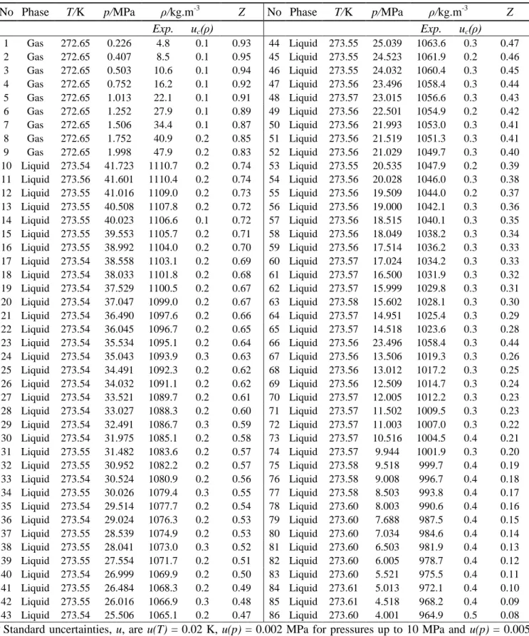
Table 3 - Experimental results of the 0.9503 mole CO2 + 0.0497 mole SO2 system at 273 K a
No Phase T/K p/MPa ρ/kg.m-3 Z No Phase T/K p/MPa ρ/kg.m-3 Z
Exp. uc(ρ) Exp. uc(ρ) 1 Gas 272.65 0.226 4.8 0.1 0.93 44 Liquid 273.55 25.039 1063.6 0.3 0.47 2 Gas 272.65 0.407 8.5 0.1 0.95 45 Liquid 273.55 24.523 1061.9 0.2 0.46 3 Gas 272.65 0.503 10.6 0.1 0.94 46 Liquid 273.55 24.032 1060.4 0.3 0.45 4 Gas 272.65 0.752 16.2 0.1 0.92 47 Liquid 273.56 23.496 1058.4 0.3 0.44 5 Gas 272.65 1.013 22.1 0.1 0.91 48 Liquid 273.57 23.015 1056.6 0.3 0.43 6 Gas 272.65 1.252 27.9 0.1 0.89 49 Liquid 273.56 22.501 1054.9 0.2 0.42 7 Gas 272.65 1.506 34.4 0.1 0.87 50 Liquid 273.56 21.993 1053.0 0.3 0.41 8 Gas 272.65 1.752 40.9 0.2 0.85 51 Liquid 273.56 21.519 1051.3 0.3 0.41 9 Gas 272.65 1.998 47.9 0.2 0.83 52 Liquid 273.56 21.029 1049.7 0.3 0.40 10 Liquid 273.54 41.723 1110.7 0.2 0.74 53 Liquid 273.55 20.535 1047.9 0.2 0.39 11 Liquid 273.56 41.601 1110.4 0.2 0.74 54 Liquid 273.56 20.028 1046.0 0.3 0.38 12 Liquid 273.55 41.016 1109.0 0.2 0.73 55 Liquid 273.56 19.509 1044.0 0.2 0.37 13 Liquid 273.55 40.508 1107.8 0.2 0.72 56 Liquid 273.56 19.000 1042.1 0.3 0.36 14 Liquid 273.55 40.023 1106.6 0.1 0.72 57 Liquid 273.56 18.515 1040.1 0.3 0.35 15 Liquid 273.55 39.553 1105.7 0.2 0.71 58 Liquid 273.56 18.049 1038.2 0.3 0.34 16 Liquid 273.55 38.992 1104.0 0.2 0.70 59 Liquid 273.56 17.514 1036.2 0.3 0.33 17 Liquid 273.54 38.558 1103.1 0.2 0.69 60 Liquid 273.57 17.024 1034.2 0.3 0.33 18 Liquid 273.54 38.033 1101.8 0.2 0.68 61 Liquid 273.57 16.500 1031.9 0.3 0.32 19 Liquid 273.54 37.529 1100.5 0.2 0.67 62 Liquid 273.57 15.999 1029.8 0.3 0.31 20 Liquid 273.54 37.047 1099.0 0.2 0.67 63 Liquid 273.58 15.602 1028.1 0.3 0.30 21 Liquid 273.54 36.490 1097.6 0.2 0.66 64 Liquid 273.57 14.951 1025.4 0.3 0.29 22 Liquid 273.54 36.045 1096.7 0.2 0.65 65 Liquid 273.57 14.518 1023.6 0.3 0.28 23 Liquid 273.54 35.534 1095.1 0.2 0.64 66 Liquid 273.56 23.496 1058.4 0.3 0.44 24 Liquid 273.54 35.043 1093.9 0.3 0.63 67 Liquid 273.56 13.506 1019.3 0.3 0.26 25 Liquid 273.54 34.491 1092.3 0.2 0.62 68 Liquid 273.56 13.012 1017.2 0.3 0.25 26 Liquid 273.54 34.032 1091.1 0.2 0.62 69 Liquid 273.56 12.509 1014.7 0.3 0.24 27 Liquid 273.54 33.521 1089.7 0.2 0.61 70 Liquid 273.57 12.005 1012.2 0.3 0.23 28 Liquid 273.54 33.027 1088.3 0.2 0.60 71 Liquid 273.57 11.502 1009.5 0.3 0.23 29 Liquid 273.54 32.491 1086.7 0.3 0.59 72 Liquid 273.57 11.003 1007.0 0.3 0.22 30 Liquid 273.54 31.975 1085.1 0.2 0.58 73 Liquid 273.57 10.516 1004.5 0.4 0.21 31 Liquid 273.55 31.482 1083.6 0.2 0.57 74 Liquid 273.57 9.944 1001.9 0.3 0.20 32 Liquid 273.55 30.952 1082.2 0.2 0.57 75 Liquid 273.58 9.518 999.7 0.4 0.19 33 Liquid 273.54 30.524 1080.9 0.2 0.56 76 Liquid 273.58 9.008 996.7 0.4 0.18 34 Liquid 273.55 30.026 1079.4 0.3 0.55 77 Liquid 273.58 8.503 993.8 0.4 0.17 35 Liquid 273.54 29.514 1077.7 0.2 0.54 78 Liquid 273.60 8.003 990.6 0.4 0.16 36 Liquid 273.54 29.024 1076.3 0.2 0.53 79 Liquid 273.60 7.688 987.5 0.4 0.15 37 Liquid 273.55 28.539 1074.9 0.2 0.53 80 Liquid 273.60 7.034 984.6 0.4 0.14 38 Liquid 273.55 28.041 1073.0 0.3 0.52 81 Liquid 273.60 6.503 981.9 0.4 0.13 39 Liquid 273.55 27.554 1071.7 0.2 0.51 82 Liquid 273.60 6.005 978.7 0.4 0.12 40 Liquid 273.54 26.999 1069.9 0.2 0.50 83 Liquid 273.60 5.521 975.5 0.4 0.11 41 Liquid 273.55 26.484 1068.3 0.2 0.49 84 Liquid 273.61 5.013 972.1 0.4 0.10 42 Liquid 273.55 26.016 1066.9 0.3 0.48 85 Liquid 273.61 4.518 968.2 0.4 0.09 43 Liquid 273.54 25.506 1065.1 0.2 0.47 86 Liquid 273.60 4.001 964.9 0.5 0.08 a
Standard uncertainties, u, are u(T) = 0.02 K, u(p) = 0.002 MPa for pressures up to 10 MPa and u(p) = 0.005 MPa for pressures from 10-40 MPa, for SO2 u(z) = 0.0001 and for CO2 u(z) = 0.0018
19
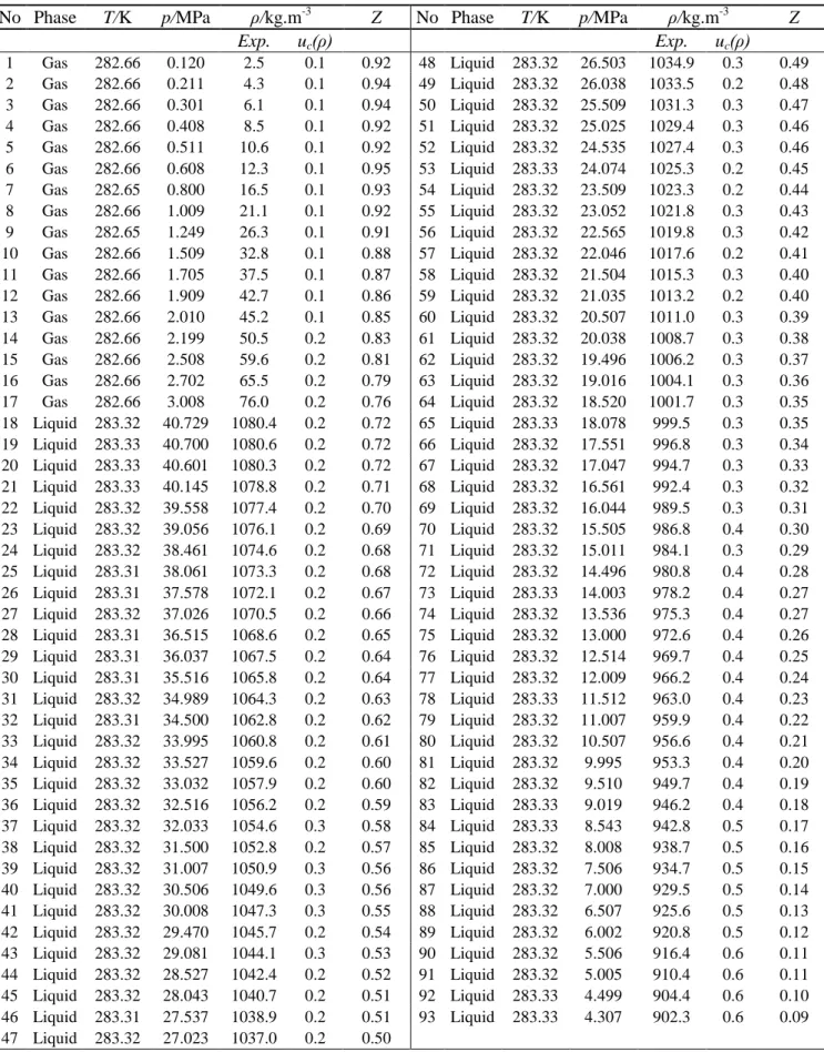
Table 4 - Experimental results of the 0.9503 mole CO2 + 0.0497 mole SO2 system at 283 K a
No Phase T/K p/MPa ρ/kg.m-3 Z No Phase T/K p/MPa ρ/kg.m-3 Z
Exp. uc(ρ) Exp. uc(ρ) 1 Gas 282.66 0.120 2.5 0.1 0.92 48 Liquid 283.32 26.503 1034.9 0.3 0.49 2 Gas 282.66 0.211 4.3 0.1 0.94 49 Liquid 283.32 26.038 1033.5 0.2 0.48 3 Gas 282.66 0.301 6.1 0.1 0.94 50 Liquid 283.32 25.509 1031.3 0.3 0.47 4 Gas 282.66 0.408 8.5 0.1 0.92 51 Liquid 283.32 25.025 1029.4 0.3 0.46 5 Gas 282.66 0.511 10.6 0.1 0.92 52 Liquid 283.32 24.535 1027.4 0.3 0.46 6 Gas 282.66 0.608 12.3 0.1 0.95 53 Liquid 283.33 24.074 1025.3 0.2 0.45 7 Gas 282.65 0.800 16.5 0.1 0.93 54 Liquid 283.32 23.509 1023.3 0.2 0.44 8 Gas 282.66 1.009 21.1 0.1 0.92 55 Liquid 283.32 23.052 1021.8 0.3 0.43 9 Gas 282.65 1.249 26.3 0.1 0.91 56 Liquid 283.32 22.565 1019.8 0.3 0.42 10 Gas 282.66 1.509 32.8 0.1 0.88 57 Liquid 283.32 22.046 1017.6 0.2 0.41 11 Gas 282.66 1.705 37.5 0.1 0.87 58 Liquid 283.32 21.504 1015.3 0.3 0.40 12 Gas 282.66 1.909 42.7 0.1 0.86 59 Liquid 283.32 21.035 1013.2 0.2 0.40 13 Gas 282.66 2.010 45.2 0.1 0.85 60 Liquid 283.32 20.507 1011.0 0.3 0.39 14 Gas 282.66 2.199 50.5 0.2 0.83 61 Liquid 283.32 20.038 1008.7 0.3 0.38 15 Gas 282.66 2.508 59.6 0.2 0.81 62 Liquid 283.32 19.496 1006.2 0.3 0.37 16 Gas 282.66 2.702 65.5 0.2 0.79 63 Liquid 283.32 19.016 1004.1 0.3 0.36 17 Gas 282.66 3.008 76.0 0.2 0.76 64 Liquid 283.32 18.520 1001.7 0.3 0.35 18 Liquid 283.32 40.729 1080.4 0.2 0.72 65 Liquid 283.33 18.078 999.5 0.3 0.35 19 Liquid 283.33 40.700 1080.6 0.2 0.72 66 Liquid 283.32 17.551 996.8 0.3 0.34 20 Liquid 283.33 40.601 1080.3 0.2 0.72 67 Liquid 283.32 17.047 994.7 0.3 0.33 21 Liquid 283.33 40.145 1078.8 0.2 0.71 68 Liquid 283.32 16.561 992.4 0.3 0.32 22 Liquid 283.32 39.558 1077.4 0.2 0.70 69 Liquid 283.32 16.044 989.5 0.3 0.31 23 Liquid 283.32 39.056 1076.1 0.2 0.69 70 Liquid 283.32 15.505 986.8 0.4 0.30 24 Liquid 283.32 38.461 1074.6 0.2 0.68 71 Liquid 283.32 15.011 984.1 0.3 0.29 25 Liquid 283.31 38.061 1073.3 0.2 0.68 72 Liquid 283.32 14.496 980.8 0.4 0.28 26 Liquid 283.31 37.578 1072.1 0.2 0.67 73 Liquid 283.33 14.003 978.2 0.4 0.27 27 Liquid 283.32 37.026 1070.5 0.2 0.66 74 Liquid 283.32 13.536 975.3 0.4 0.27 28 Liquid 283.31 36.515 1068.6 0.2 0.65 75 Liquid 283.32 13.000 972.6 0.4 0.26 29 Liquid 283.31 36.037 1067.5 0.2 0.64 76 Liquid 283.32 12.514 969.7 0.4 0.25 30 Liquid 283.31 35.516 1065.8 0.2 0.64 77 Liquid 283.32 12.009 966.2 0.4 0.24 31 Liquid 283.32 34.989 1064.3 0.2 0.63 78 Liquid 283.33 11.512 963.0 0.4 0.23 32 Liquid 283.31 34.500 1062.8 0.2 0.62 79 Liquid 283.32 11.007 959.9 0.4 0.22 33 Liquid 283.32 33.995 1060.8 0.2 0.61 80 Liquid 283.32 10.507 956.6 0.4 0.21 34 Liquid 283.32 33.527 1059.6 0.2 0.60 81 Liquid 283.32 9.995 953.3 0.4 0.20 35 Liquid 283.32 33.032 1057.9 0.2 0.60 82 Liquid 283.32 9.510 949.7 0.4 0.19 36 Liquid 283.32 32.516 1056.2 0.2 0.59 83 Liquid 283.33 9.019 946.2 0.4 0.18 37 Liquid 283.32 32.033 1054.6 0.3 0.58 84 Liquid 283.33 8.543 942.8 0.5 0.17 38 Liquid 283.32 31.500 1052.8 0.2 0.57 85 Liquid 283.32 8.008 938.7 0.5 0.16 39 Liquid 283.32 31.007 1050.9 0.3 0.56 86 Liquid 283.32 7.506 934.7 0.5 0.15 40 Liquid 283.32 30.506 1049.6 0.3 0.56 87 Liquid 283.32 7.000 929.5 0.5 0.14 41 Liquid 283.32 30.008 1047.3 0.3 0.55 88 Liquid 283.32 6.507 925.6 0.5 0.13 42 Liquid 283.32 29.470 1045.7 0.2 0.54 89 Liquid 283.32 6.002 920.8 0.5 0.12 43 Liquid 283.32 29.081 1044.1 0.3 0.53 90 Liquid 283.32 5.506 916.4 0.6 0.11 44 Liquid 283.32 28.527 1042.4 0.2 0.52 91 Liquid 283.32 5.005 910.4 0.6 0.11 45 Liquid 283.32 28.043 1040.7 0.2 0.51 92 Liquid 283.33 4.499 904.4 0.6 0.10 46 Liquid 283.31 27.537 1038.9 0.2 0.51 93 Liquid 283.33 4.307 902.3 0.6 0.09 47 Liquid 283.32 27.023 1037.0 0.2 0.50 a
Standard uncertainties, u, are u(T) = 0.02 K, u(p) = 0.002 MPa for pressures up to 10 MPa and u(p) = 0.005 MPa for pressures from 10-40 MPa, for SO2 u(z) = 0.0001 and for CO2 u(z) = 0.0018
20
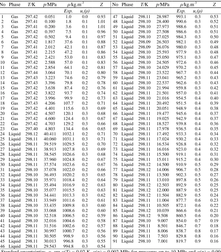
Table 5 - Experimental results of the 0.9478 mole CO2 + 0.0522 mole SO2 system at 298 K a
No Phase T/K p/MPa ρ/kg.m-3 Z No Phase T/K p/MPa ρ/kg.m-3 Z
Exp. uc(ρ) Exp. uc(ρ) 1 Gas 297.42 0.051 1.0 0.0 0.93 47 Liquid 298.11 28.987 993.1 0.3 0.53 2 Gas 297.41 0.100 1.8 0.1 1.01 48 Liquid 298.10 28.400 990.6 0.3 0.52 3 Gas 297.41 0.200 3.6 0.1 1.01 49 Liquid 298.10 27.973 988.6 0.3 0.51 4 Gas 297.42 0.397 7.5 0.1 0.96 50 Liquid 298.10 27.508 986.6 0.3 0.51 5 Gas 297.42 0.502 9.4 0.1 0.97 51 Liquid 298.10 27.025 984.3 0.3 0.50 6 Gas 297.42 1.817 37.6 0.1 0.88 52 Liquid 298.09 26.503 982.1 0.3 0.49 7 Gas 297.41 2.012 42.1 0.1 0.87 53 Liquid 298.09 26.076 980.0 0.3 0.48 8 Gas 297.41 2.215 47.2 0.1 0.86 54 Liquid 298.10 25.593 977.9 0.3 0.48 9 Gas 297.42 2.421 53.0 0.1 0.83 55 Liquid 298.10 25.050 975.1 0.3 0.47 10 Gas 297.42 2.588 57.0 0.1 0.83 56 Liquid 298.10 24.505 972.6 0.3 0.46 11 Gas 297.42 2.854 64.1 0.2 0.81 57 Liquid 298.10 24.029 970.2 0.3 0.45 12 Gas 297.44 3.064 70.1 0.2 0.80 58 Liquid 298.10 23.522 967.7 0.3 0.44 13 Gas 297.43 3.223 74.6 0.2 0.79 59 Liquid 298.11 23.041 965.2 0.3 0.43 14 Gas 297.43 3.396 79.8 0.2 0.78 60 Liquid 298.10 22.537 962.6 0.3 0.43 15 Gas 297.42 3.638 87.4 0.2 0.76 61 Liquid 298.10 21.994 959.8 0.3 0.42 16 Gas 297.42 3.822 93.7 0.2 0.74 62 Liquid 298.11 21.501 957.0 0.3 0.41 17 Gas 297.42 3.996 99.9 0.2 0.73 63 Liquid 298.10 21.016 954.5 0.4 0.40 18 Gas 297.43 4.206 107.7 0.2 0.71 64 Liquid 298.11 20.492 951.5 0.4 0.39 19 Gas 297.42 4.401 115.6 0.3 0.69 65 Liquid 298.11 20.051 948.9 0.4 0.38 20 Gas 297.42 4.507 120.1 0.3 0.68 66 Liquid 298.11 19.477 945.6 0.4 0.37 21 Gas 297.42 4.600 124.4 0.3 0.67 67 Liquid 298.11 19.025 942.9 0.4 0.37 22 Gas 297.42 4.703 129.2 0.3 0.66 68 Liquid 298.11 18.527 939.8 0.4 0.36 23 Gas 297.40 4.803 134.4 0.6 0.65 69 Liquid 298.11 17.978 936.5 0.4 0.35 24 Liquid 298.12 40.411 1032.1 0.2 0.71 70 Liquid 298.11 17.492 933.3 0.4 0.34 25 Liquid 298.11 40.060 1031.1 0.3 0.71 71 Liquid 298.11 17.024 930.2 0.4 0.33 26 Liquid 298.11 39.519 1029.5 0.2 0.70 72 Liquid 298.11 16.534 926.8 0.4 0.32 27 Liquid 298.11 38.913 1027.8 0.3 0.69 73 Liquid 298.11 16.016 923.0 0.4 0.32 28 Liquid 298.11 38.545 1026.6 0.3 0.68 74 Liquid 298.11 15.500 919.1 0.4 0.31 29 Liquid 298.11 37.960 1024.8 0.2 0.67 75 Liquid 298.11 15.011 915.2 0.4 0.30 30 Liquid 298.11 37.574 1023.6 0.2 0.67 76 Liquid 298.12 14.500 910.9 0.5 0.29 31 Liquid 298.10 37.078 1022.0 0.2 0.66 77 Liquid 298.12 14.006 906.7 0.5 0.28 32 Liquid 298.10 36.493 1020.2 0.3 0.65 78 Liquid 298.11 13.500 902.3 0.5 0.27 33 Liquid 298.10 35.971 1018.4 0.2 0.64 79 Liquid 298.11 13.010 897.8 0.5 0.26 34 Liquid 298.11 35.494 1016.9 0.2 0.63 80 Liquid 298.12 12.503 892.9 0.5 0.25 35 Liquid 298.10 35.077 1015.5 0.2 0.63 81 Liquid 298.12 12.000 887.9 0.5 0.25 36 Liquid 298.10 34.441 1013.3 0.3 0.62 82 Liquid 298.12 11.504 882.9 0.5 0.24 37 Liquid 298.11 33.949 1011.6 0.2 0.61 83 Liquid 298.11 11.004 877.7 0.6 0.23 38 Liquid 298.10 33.435 1009.8 0.3 0.60 84 Liquid 298.11 10.505 872.1 0.6 0.22 39 Liquid 298.10 33.068 1008.6 0.2 0.60 85 Liquid 298.12 10.039 866.6 0.6 0.21 40 Liquid 298.10 32.518 1006.5 0.2 0.59 86 Liquid 298.12 9.508 860.5 0.6 0.20 41 Liquid 298.10 32.016 1004.6 0.2 0.58 87 Liquid 298.10 9.007 854.0 0.7 0.19 42 Liquid 298.11 31.516 1002.6 0.2 0.57 88 Liquid 298.11 8.501 846.7 0.7 0.18 43 Liquid 298.11 30.997 1000.7 0.2 0.56 89 Liquid 298.11 8.006 838.7 0.8 0.17 44 Liquid 298.11 30.505 998.9 0.3 0.56 90 Liquid 298.11 7.503 829.8 0.8 0.16 45 Liquid 298.11 30.013 996.8 0.3 0.55 91 Liquid 298.10 7.001 819.7 0.9 0.16 46 Liquid 298.11 29.543 994.8 0.3 0.54 a
Standard uncertainties, u, are u(T) = 0.02 K, u(p) = 0.002 MPa for pressures up to 10 MPa and u(p) = 0.005 MPa for pressures from 10-40 MPa, for SO2 u(z) = 0.0001 and for CO2 u(z) = 0.0018
21
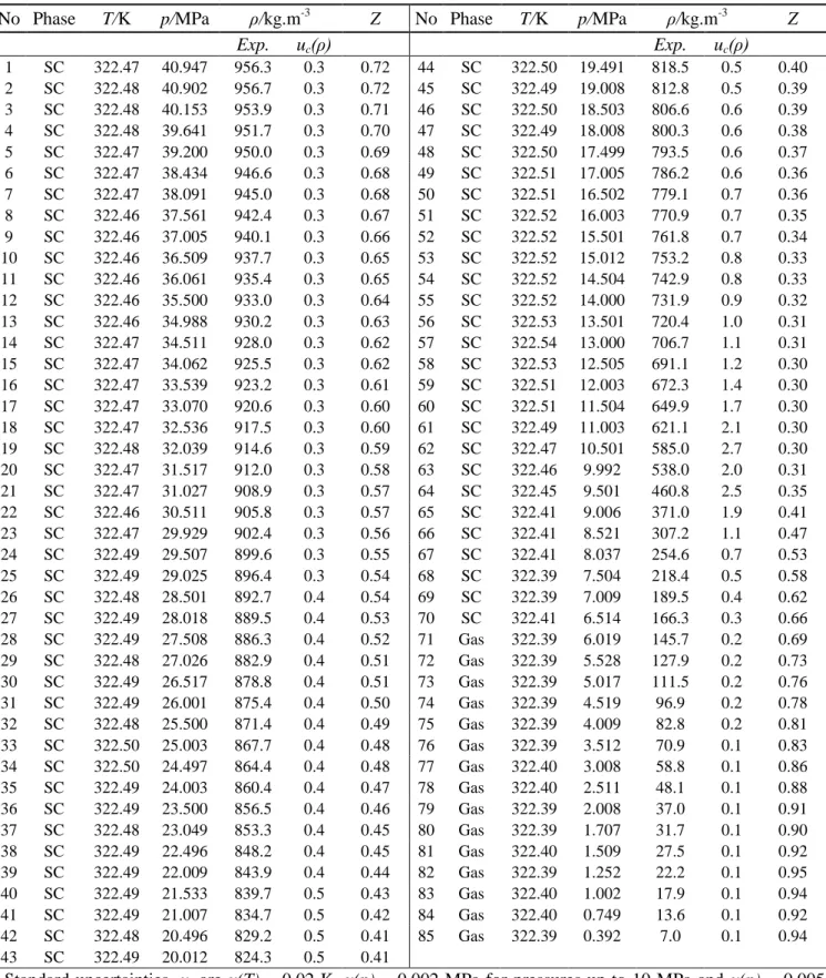
Table 6 - Experimental results of the 0.9503 mole CO2 + 0.0497 mole SO2 system at 323 K a
No Phase T/K p/MPa ρ/kg.m-3 Z No Phase T/K p/MPa ρ/kg.m-3 Z
Exp. uc(ρ) Exp. uc(ρ) 1 SC 322.47 40.947 956.3 0.3 0.72 44 SC 322.50 19.491 818.5 0.5 0.40 2 SC 322.48 40.902 956.7 0.3 0.72 45 SC 322.49 19.008 812.8 0.5 0.39 3 SC 322.48 40.153 953.9 0.3 0.71 46 SC 322.50 18.503 806.6 0.6 0.39 4 SC 322.48 39.641 951.7 0.3 0.70 47 SC 322.49 18.008 800.3 0.6 0.38 5 SC 322.47 39.200 950.0 0.3 0.69 48 SC 322.50 17.499 793.5 0.6 0.37 6 SC 322.47 38.434 946.6 0.3 0.68 49 SC 322.51 17.005 786.2 0.6 0.36 7 SC 322.47 38.091 945.0 0.3 0.68 50 SC 322.51 16.502 779.1 0.7 0.36 8 SC 322.46 37.561 942.4 0.3 0.67 51 SC 322.52 16.003 770.9 0.7 0.35 9 SC 322.46 37.005 940.1 0.3 0.66 52 SC 322.52 15.501 761.8 0.7 0.34 10 SC 322.46 36.509 937.7 0.3 0.65 53 SC 322.52 15.012 753.2 0.8 0.33 11 SC 322.46 36.061 935.4 0.3 0.65 54 SC 322.52 14.504 742.9 0.8 0.33 12 SC 322.46 35.500 933.0 0.3 0.64 55 SC 322.52 14.000 731.9 0.9 0.32 13 SC 322.46 34.988 930.2 0.3 0.63 56 SC 322.53 13.501 720.4 1.0 0.31 14 SC 322.47 34.511 928.0 0.3 0.62 57 SC 322.54 13.000 706.7 1.1 0.31 15 SC 322.47 34.062 925.5 0.3 0.62 58 SC 322.53 12.505 691.1 1.2 0.30 16 SC 322.47 33.539 923.2 0.3 0.61 59 SC 322.51 12.003 672.3 1.4 0.30 17 SC 322.47 33.070 920.6 0.3 0.60 60 SC 322.51 11.504 649.9 1.7 0.30 18 SC 322.47 32.536 917.5 0.3 0.60 61 SC 322.49 11.003 621.1 2.1 0.30 19 SC 322.48 32.039 914.6 0.3 0.59 62 SC 322.47 10.501 585.0 2.7 0.30 20 SC 322.47 31.517 912.0 0.3 0.58 63 SC 322.46 9.992 538.0 2.0 0.31 21 SC 322.47 31.027 908.9 0.3 0.57 64 SC 322.45 9.501 460.8 2.5 0.35 22 SC 322.46 30.511 905.8 0.3 0.57 65 SC 322.41 9.006 371.0 1.9 0.41 23 SC 322.47 29.929 902.4 0.3 0.56 66 SC 322.41 8.521 307.2 1.1 0.47 24 SC 322.49 29.507 899.6 0.3 0.55 67 SC 322.41 8.037 254.6 0.7 0.53 25 SC 322.49 29.025 896.4 0.3 0.54 68 SC 322.39 7.504 218.4 0.5 0.58 26 SC 322.48 28.501 892.7 0.4 0.54 69 SC 322.39 7.009 189.5 0.4 0.62 27 SC 322.49 28.018 889.5 0.4 0.53 70 SC 322.41 6.514 166.3 0.3 0.66 28 SC 322.49 27.508 886.3 0.4 0.52 71 Gas 322.39 6.019 145.7 0.2 0.69 29 SC 322.48 27.026 882.9 0.4 0.51 72 Gas 322.39 5.528 127.9 0.2 0.73 30 SC 322.49 26.517 878.8 0.4 0.51 73 Gas 322.39 5.017 111.5 0.2 0.76 31 SC 322.49 26.001 875.4 0.4 0.50 74 Gas 322.39 4.519 96.9 0.2 0.78 32 SC 322.48 25.500 871.4 0.4 0.49 75 Gas 322.39 4.009 82.8 0.2 0.81 33 SC 322.50 25.003 867.7 0.4 0.48 76 Gas 322.39 3.512 70.9 0.1 0.83 34 SC 322.50 24.497 864.4 0.4 0.48 77 Gas 322.40 3.008 58.8 0.1 0.86 35 SC 322.49 24.003 860.4 0.4 0.47 78 Gas 322.40 2.511 48.1 0.1 0.88 36 SC 322.49 23.500 856.5 0.4 0.46 79 Gas 322.39 2.008 37.0 0.1 0.91 37 SC 322.48 23.049 853.3 0.4 0.45 80 Gas 322.39 1.707 31.7 0.1 0.90 38 SC 322.49 22.496 848.2 0.4 0.45 81 Gas 322.40 1.509 27.5 0.1 0.92 39 SC 322.49 22.009 843.9 0.4 0.44 82 Gas 322.39 1.252 22.2 0.1 0.95 40 SC 322.49 21.533 839.7 0.5 0.43 83 Gas 322.40 1.002 17.9 0.1 0.94 41 SC 322.49 21.007 834.7 0.5 0.42 84 Gas 322.40 0.749 13.6 0.1 0.92 42 SC 322.48 20.496 829.2 0.5 0.41 85 Gas 322.39 0.392 7.0 0.1 0.94 43 SC 322.49 20.012 824.3 0.5 0.41 a
Standard uncertainties, u, are u(T) = 0.02 K, u(p) = 0.002 MPa for pressures up to 10 MPa and u(p) = 0.005 MPa for pressures from 10-40 MPa, for SO2 u(z) = 0.0001 and for CO2 u(z) = 0.0018
22
Table 7 - Experimental results of the 0.9503 mole CO2 + 0.0497 mole SO2 system at 353 K a
No Phase T/K p/MPa ρ/kg.m-3 Z No Phase T/K p/MPa ρ/kg.m-3 Z
Exp. uc(ρ) Exp. uc(ρ) 1 SC 352.98 39.330 850.5 0.3 0.71 45 SC 352.97 18.007 583.3 1.0 0.47 2 SC 352.98 39.300 850.2 0.3 0.71 46 SC 352.95 17.520 569.4 1.0 0.47 3 SC 352.97 39.009 848.1 0.3 0.71 47 SC 352.96 17.006 552.6 1.1 0.47 4 SC 352.97 38.520 845.7 0.3 0.70 48 SC 352.95 16.515 535.1 1.2 0.47 5 SC 352.98 38.023 842.1 0.3 0.69 49 SC 352.96 16.004 514.7 1.2 0.48 6 SC 352.97 37.499 838.7 0.3 0.69 50 SC 352.95 15.497 493.2 1.3 0.48 7 SC 352.96 36.996 835.2 0.3 0.68 51 SC 352.96 15.003 470.1 1.4 0.49 8 SC 352.97 36.496 831.8 0.3 0.67 52 SC 352.95 14.502 447.3 1.4 0.50 9 SC 352.98 36.013 828.1 0.3 0.67 53 SC 352.96 14.004 422.3 1.4 0.51 10 SC 352.97 35.510 824.7 0.3 0.66 54 SC 352.96 13.501 397.6 1.4 0.52 11 SC 352.97 35.014 821.4 0.4 0.65 55 SC 352.96 12.998 371.8 1.4 0.54 12 SC 352.98 34.563 818.1 0.4 0.65 56 SC 352.95 12.505 346.8 1.4 0.55 13 SC 352.97 34.055 814.5 0.4 0.64 57 SC 352.95 12.000 321.9 1.3 0.57 14 SC 352.96 33.519 809.8 0.4 0.63 58 SC 352.97 11.505 298.8 1.2 0.59 15 SC 352.96 33.014 805.8 0.4 0.63 59 SC 352.96 11.001 276.4 1.1 0.61 16 SC 352.97 32.552 802.4 0.4 0.62 60 SC 352.97 10.506 255.3 1.0 0.63 17 SC 352.96 31.993 797.6 0.4 0.62 61 SC 352.96 10.075 238.1 1.0 0.65 18 SC 352.95 31.494 793.2 0.4 0.61 62 SC 352.95 9.230 209.5 0.3 0.68 19 SC 352.96 31.058 789.4 0.4 0.60 63 SC 352.94 9.008 201.9 0.3 0.68 20 SC 352.97 30.512 784.7 0.4 0.60 64 SC 352.96 8.507 185.5 0.2 0.70 21 SC 352.96 29.991 779.0 0.4 0.59 65 SC 352.94 8.038 170.3 0.2 0.72 22 SC 352.96 29.492 773.9 0.4 0.58 66 SC 352.94 7.498 154.1 0.2 0.75 23 SC 352.97 29.001 768.7 0.4 0.58 67 Gas 352.94 7.017 140.9 0.2 0.76 24 SC 352.96 28.507 764.2 0.5 0.57 68 Gas 352.94 6.516 127.7 0.2 0.78 25 SC 352.96 28.006 758.3 0.5 0.57 69 Gas 352.93 6.001 114.8 0.2 0.80 26 SC 352.96 27.501 752.6 0.5 0.56 70 Gas 352.95 5.490 102.6 0.2 0.82 27 SC 352.98 27.043 747.4 0.5 0.55 71 Gas 352.95 4.997 91.5 0.1 0.84 28 SC 352.97 26.597 742.8 0.5 0.55 72 Gas 352.94 4.493 80.5 0.1 0.86 29 SC 352.96 26.036 736.4 0.5 0.54 73 Gas 352.94 4.003 70.6 0.1 0.87 30 SC 352.96 25.555 731.2 0.5 0.54 74 Gas 352.96 3.495 60.3 0.1 0.89 31 SC 352.95 25.002 723.7 0.5 0.53 75 Gas 352.95 3.009 51.0 0.1 0.90 32 SC 352.95 24.538 717.4 0.6 0.52 76 Gas 352.95 2.800 47.2 0.1 0.91 33 SC 352.96 24.023 710.4 0.6 0.52 77 Gas 352.94 2.504 41.8 0.1 0.92 34 SC 352.96 23.524 703.1 0.6 0.51 78 Gas 352.95 2.248 37.0 0.1 0.93 35 SC 352.95 23.011 694.8 0.6 0.51 79 Gas 352.95 2.002 33.0 0.1 0.93 36 SC 352.95 22.493 686.4 0.6 0.50 80 Gas 352.94 1.742 28.6 0.1 0.93 37 SC 352.95 21.993 677.2 0.7 0.50 81 Gas 352.95 1.507 24.3 0.1 0.95 38 SC 352.96 21.521 668.5 0.7 0.49 82 Gas 352.96 1.248 19.9 0.1 0.96 39 SC 352.96 20.999 657.9 0.7 0.49 83 Gas 352.96 0.982 15.1 0.1 1.00 40 SC 352.96 20.490 647.4 0.8 0.49 84 Gas 352.95 0.740 11.4 0.1 1.00 41 SC 352.96 20.014 636.9 0.8 0.48 85 Gas 352.95 0.511 7.6 0.1 1.03 42 SC 352.95 19.511 624.5 0.8 0.48 86 Gas 352.95 0.402 6.0 0.1 1.03 43 SC 352.96 19.011 611.7 0.9 0.48 87 Gas 352.95 0.306 4.6 0.1 1.02 44 SC 352.97 18.500 597.8 0.9 0.47 88 Gas 352.93 0.202 3.0 0.1 1.03 a
Standard uncertainties, u, are u(T) = 0.02 K, u(p) = 0.002 MPa for pressures up to 10 MPa and u(p) = 0.005 MPa for pressures from 10-40 MPa, for SO2 u(z) = 0.0001 and for CO2 u(z) = 0.0018
23
Table 8 - Uncertainties with 95% level of confidence (k=2) for the measured densities of the CO2-SO2
system
Uncertainties U()
T / K Phase Data Average Max.
No. kg.m-3 % kg.m-3 % 273 Gas 9 0.2 0.7 0.3 2.2 Liquid 77 0.3 0.0 0.5 0.1 SC 0 0.0 0.0 0.0 1.0 Total 86 0.3 0.1 0.5 2.2 283 Gas 17 0.2 0.8 0.7 4.1 Liquid 76 0.3 0.0 0.6 0.1 SC 0 0.0 1.0 0.0 1.0 Total 93 0.3 0.2 0.7 4.1 298 Gas 23 0.3 0.7 1.2 4.4 Liquid 68 0.4 0.0 0.9 0.1 SC 0 0.0 1.0 0.0 1.0 Total 91 0.3 0.2 1.2 4.4 323 Gas 15 0.1 0.4 0.2 1.4 Liquid 0 0.0 1.0 0.0 1.0 SC 70 0.6 0.1 2.7 0.6 Total 85 0.5 0.2 2.7 1.4 353 Gas 22 0.1 0.6 0.2 2.9 Liquid 0 0.0 1.0 0.0 1.0 SC 66 0.7 0.1 1.4 0.4 Total 88 0.5 0.2 1.4 2.9 Total Gas 86 0.2 0.6 1.2 4.4 Liquid 221 0.3 0.03 0.9 1.0 SC 136 0.6 0.12 2.7 1.0 Total 443 0.4 0.2 2.7 4.4
24
Table 9 - Summarised AADs for the measured density of the CO2-SO2 system
Gas Liquid SC Overall
No of Exp. Data 86 221 136 443 Average SRK 2.4 8.2 9.6 7.4 Absolute PR 1.8 3.2 2.4 2.6 Deviation VPT 1.8 1.9 2.6 2.1 (%) SRK-CO2 1.9 0.6 0.8 1.0 PR-CO2 1.7 0.7 1.1 1.0 VPT-CO2 2.2 0.7 1.1 1.1 SRK-Peneloux 1.9 1.6 4.6 2.6 PR-Peneloux 1.9 1.1 3.8 2.1
Multi parameter EoS 1.6 0.2 0.6 0.6
Maximum SRK 13.1 14.6 15.2 15.2 Absolute PR 7.3 7.6 7.3 7.6 Deviation VPT 7.3 8.0 7.5 8.0 (%) SRK-CO2 7.4 8.0 6.3 8.0 PR-CO2 7.4 7.1 5.8 7.4 VPT-CO2 7.4 7.2 5.6 7.4 SRK-Peneloux 8.5 9.3 11.9 11.9 PR-Peneloux 7.3 8.0 9.2 9.2
25
Table 10 - Specific heat capacity calculations for the CO2 – SO2 system a T/K p/MPa ρ/ kg.m-3 ν/ (m3.mol-1) Cp 0 / (J.K-1.mol-1) CpExp/ (J.K-1.mol-1) U(Cp)/ (J.K-1.mol-1) CpMP/ (J.K-1.mol-1) Dev./(%) 40 MPa 273.55 40.023 1106.61 4.0671E-05 36.08 76.66 0.14 77.75 1.4 283.33 40.145 1078.76 4.1721E-05 36.34 76.54 0.15 77.88 1.8 298.11 40.060 1031.14 4.3648E-05 37.08 76.92 0.16 78.25 1.7 322.48 40.153 953.87 4.7184E-05 38.25 77.63 0.17 79.25 2.1 352.98 39.330 850.47 5.292E-05 39.58 78.39 0.18 80.78 3.1 35 MPa 273.54 35.043 1093.91 4.1143E-05 35.83 80.66 0.17 78.90 -2.2 283.32 34.989 1064.30 4.2288E-05 36.34 81.21 0.18 79.29 -2.4 298.10 35.077 1015.50 4.432E-05 37.08 82.07 0.19 79.98 -2.5 322.46 34.988 930.22 4.8383E-05 38.25 83.86 0.20 81.85 -2.4 352.97 35.014 821.42 5.4792E-05 39.58 85.51 0.21 83.87 -1.9 30 MPa 273.55 30.026 1079.37 4.1697E-05 35.83 82.95 0.20 80.32 -3.2 283.32 30.008 1047.27 4.2976E-05 36.34 83.82 0.21 81.00 -3.4 298.11 30.013 996.85 4.5149E-05 37.08 85.34 0.22 82.27 -3.6 322.47 29.929 902.37 4.9877E-05 38.25 88.50 0.24 85.43 -3.5 352.96 29.991 778.96 5.7779E-05 39.58 91.81 0.24 89.08 -3.0 25 MPa 273.55 25.039 1063.62 4.3152E-05 35.83 87.42 0.26 82.09 -6.1 283.32 25.025 1029.35 4.4009E-05 36.34 88.89 0.28 83.20 -6.4 298.10 25.050 975.15 4.6687E-05 37.08 91.66 0.29 85.32 -6.9 322.50 25.003 867.65 5.3224E-05 38.26 97.26 0.31 90.70 -6.7 352.95 25.002 723.72 6.4973E-05 39.58 103.82 0.30 97.64 -6.0 20 MPa 273.56 20.028 1046.04 4.3026E-05 35.83 91.74 0.42 84.42 -8.0 283.32 20.038 1008.74 4.4617E-05 36.34 93.99 0.43 86.19 -8.3 298.11 20.051 948.90 4.7431E-05 37.08 98.42 0.45 89.81 -8.7 322.49 20.012 824.32 5.4599E-05 38.26 109.99 0.46 99.90 -9.2 352.96 20.014 636.90 7.0666E-05 39.58 121.49 0.42 114.42 -5.8 15 MPa 273.57 14.951 1025.38 4.3893E-05 35.83 102.28 0.92 87.64 -14.3 283.32 15.011 984.11 4.5734E-05 36.34 106.18 0.94 90.58 -14.7 298.11 15.011 915.17 4.9179E-05 37.08 115.12 0.94 97.28 -15.5 322.52 15.012 753.20 5.9754E-05 38.26 146.76 0.90 121.74 -17.0 352.96 15.003 470.12 9.5734E-05 39.58 143.82 0.98 141.94 -1.3 AAD (%) 0.37 5.8 a
26
Table 11 - Estimated bubble points from the measured densities for the CO2 - SO2 system a
Type Experimental Prediction (PR-CO2) Deviations (%)
T/K p/MPa ρ/ kg.m-3 uc(ρ)/ kg.m-3 p/MPa ρ/ kg.m -3 p ρ Bubble Point 273.56 3.484 964.4 0.5 3.303 976.4 -5.2 1.2 Bubble Point 283.33 4.304 908.4 0.6 4.221 929.2 -1.9 2.3
Absolute Average Deviation (AAD) (%) 3.6 1.8
a
27
Figure 1 - Schematic diagram of the densitometer apparatus
1) Anton Paar DMA 512 densitometer, 2) High pressure fluid vessel, 3) Capillary Valve , 4) Liquid bath (model: Lauda RE206), 5) Liquid bath of circuit (model: West P6100), 6) Pressure transducers (model: Druck PTX611), 7) Temperature probes, 8) Vacuum pump, 9) Neutralisation column, 10) Data acquisition unit, V1) Circuit valve, V2) Flow controlling ball
28
Figure 2 -Experimental and predicted densities of the CO2 – SO2 system. Experimental results: (∆)
273. 15 K, (*) 283.15 K, (◊) 323.15 K and (□) 353.15 K for the 0.9503 mole CO2 + 0.0497 mole SO2
and (○) 298.15 K for the 0.9478 mole CO2 + 0.0522 mole SO2. Lines: Predictions using the multi
parameter EoS
0
200
400
600
800
1000
1200
0
10
20
30
40
ρ
/k
g.
m
-3p/MPa
29
Figure 3 – Low pressure experimental and predicted densities of the CO2 – SO2 system. Experimental
results: (∆) 273. 15 K, (*) 283.15 K, (◊) 323.15 K and (□) 353.15 K for the 0.9503 mole CO2 + 0.0497
mole SO2 and (○) 298.15 K for the 0.9478 mole CO2 + 0.0522 mole SO2. Lines: Predictions using the
multi parameter EoS
0
20
40
60
80
100
120
140
160
180
200
0
2
4
6
8
ρ
/k
g.
m
-3p/MPa
30
Figure 4 – Deviations of the predictions using the multi parameter EoS from the measured data, (∆) 273. 15 K, (*) 283.15 K, (◊) 323.15 K and (□) 353.15 K for the 0.9503 mole CO2 + 0.0497 mole SO2
and (○) 298.15 K for the 0.9478 mole CO2 + 0.0522 mole SO2.
-5.0
-3.0
-1.0
1.0
3.0
5.0
7.0
0
10
20
30
40
(ρ
PR -CO 2-ρ
Ex p)/
ρ
Ex p100
p/MPa
31
Figure 5 – Compressibility factor of the CO2 – SO2 system.
Experimental results: (∆) 273. 15 K, (*) 283.15 K, (◊) 323.15 K and (□) 353.15 K for the 0.9503 mole CO2 + 0.0497 mole SO2 and (○) 298.15 K for the 0.9478 mole CO2 + 0.0522 mole SO2. Lines:
Predictions using the multi parameter EoS
0.0
0.1
0.2
0.3
0.4
0.5
0.6
0.7
0.8
0.9
1.0
0
10
20
30
40
Z-Fact
or
p/MPa
32
Figure 6 – Compressibility factor of the CO2 – SO2 system.
Experimental results: (∆) 273. 15 K, (*) 283.15 K, (◊) 323.15 K and (□) 353.15 K for the 0.9503 mole CO2 + 0.0497 mole SO2 and (○) 298.15 K for the 0.9478 mole CO2 + 0.0522 mole SO2. Lines:
Predictions using the multi parameter EoS
0.50
0.55
0.60
0.65
0.70
0.75
0.80
0.85
0.90
0.95
1.00
0
2
4
6
8
10
Z-Fact
or
p/MPa
33
Figure 7 - Specific heat capacity of the CO2 – SO2 system (0.9503 mole CO2 + 0.0497 mole SO2 at
273. 15 K, 283.15 K, 323.15 K and 353.15 K and 0.9478 mole CO2 + 0.0522 mole SO2 at 298.15 K):
(●) calculated Cp with 3% error, Lines: predictions using the multi parameter EoS
70 75 80 85 90 95 100 270 290 310 330 350 370 Cp / (J .K -1.m ol -1) T / K 40 MPa 70 75 80 85 90 95 100 270 290 310 330 350 370 Cp / (J .K -1.m ol -1) T / K 35 MPa 70 75 80 85 90 95 100 270 290 310 330 350 370 Cp / (J .K -1.m ol -1) T / K 30 MPa 70 75 80 85 90 95 100 105 110 270 290 310 330 350 370 Cp / (J .K -1.m ol -1) T / K 25 MPa 80 85 90 95 100 105 110 115 120 125 130 270 290 310 330 350 370 Cp / (J .K -1.m ol -1) T / K 20 MPa 80 90 100 110 120 130 140 150 160 270 290 310 330 350 370 Cp / (J .K -1.m ol -1) T / K 15 MPa
34
Figure 8 – Bubble point determination of 0.9503 mole CO2 + 0.0497 mole SO2 system for different
isotherms, (∆) 273. 15 K, (*) 283.15 K

![Table 2 - Constants B to F in the Aly & Lee equation [45]](https://thumb-eu.123doks.com/thumbv2/123doknet/11645391.307715/18.892.130.764.141.220/table-constants-b-f-aly-amp-lee-equation.webp)