HAL Id: hal-01153274
https://hal-enpc.archives-ouvertes.fr/hal-01153274
Submitted on 4 Jul 2018
HAL is a multi-disciplinary open access
archive for the deposit and dissemination of
sci-entific research documents, whether they are
pub-lished or not. The documents may come from
teaching and research institutions in France or
abroad, or from public or private research centers.
L’archive ouverte pluridisciplinaire HAL, est
destinée au dépôt et à la diffusion de documents
scientifiques de niveau recherche, publiés ou non,
émanant des établissements d’enseignement et de
recherche français ou étrangers, des laboratoires
publics ou privés.
Match Selection and Refinement for Highly Accurate
Two-View Structure from Motion
Zhe Liu, Pascal Monasse, Renaud Marlet
To cite this version:
Zhe Liu, Pascal Monasse, Renaud Marlet. Match Selection and Refinement for Highly Accurate
Two-View Structure from Motion. ECCV 2014 ( European Conference on Computer Vision 2014), Sep
2014, Zurich, Switzerland. pp.818-833, �10.1007/978-3-319-10605-2_53�. �hal-01153274�
Accurate Two-View Structure from Motion
Zhe Liu, Pascal Monasse, and Renaud Marlet
Universit´e Paris-Est, LIGM (UMR 8049), ENPC, F-77455 Marne-la-Vall´ee, France
Abstract. We present an approach to enhance the accuracy of structure from motion (SfM) in the two-view case. We first answer the question: “fewer data with higher accuracy, or more data with less accuracy?” For this, we establish a relation between SfM errors and a function of the number of matches and their epipolar errors. Using an accuracy estima-tor of individual matches, we then propose a method to select a subset of matches that has a good quality vs. quantity compromise. We also pro-pose a variant of least squares matching to refine match locations based on a focused grid and a multi-scale exploration. Experiments show that both selection and refinement contribute independently to a better ac-curacy. Their combination reduces errors by a factor of 1.1 to 2.0 for rotation, and 1.6 to 3.8 for translation.
1
Introduction
3D reconstructions from pictures are increasingly being used to model real scenes or objects. For some applications such as video games or virtual film sets, cap-turing the general shape and appearance is enough. The reconstruction method does not have to be particularly accurate. However, in industrial settings, where 3D models are used for measurement, accuracy is crucial. Moreover, even for less demanding tasks, accurate reconstruction reduces the quantity of required images, thus reducing the costs and increasing the applicability. Better estimates also lessen the impact of outliers.
In this paper, we propose a method to greatly enhance the accuracy of two-view structure from motion (SfM), i.e., the estimation of the camera poses (posi-tions and orienta(posi-tions) and of the basic structure of the scene (3D point cloud). As 3D reconstruction methods strongly rely on the quality of the estimated cal-ibration, this is a crucial initial step. In most cases, being wrong at calibration time cannot be recovered later.
Match selection. Most SfM approaches are based on the detection and match-ing of interest points (features) in image pairs [11]. Given point matches between two images, we can estimate a fundamental matrix F relating them. If internal calibration parameters are known (calibration matrix K), this also provides an estimate of the camera motion (rotation R, translation t) and 3D position of matched points. As feature detection and matching is not perfect, two main things can go wrong in the SfM process: the matches can be either incorrect
or inaccurate. There is actually a grey area between these notions: incorrect matches reduce SfM accuracy, sometimes to the point of making it fail, while inaccurate matches are considered as good enough for calibrating, even though they also degrade SfM accuracy. Incorrect matches are generally dealt with us-ing RANSAC [9] or one of its numerous variants [7, 8, 19, 26]. It separates “good matches” (inliers) from “wrong matches” (outliers), trying to find the largest consensus on an estimated fundamental matrix, using a threshold (fixed or adap-tive) to assess consistency. While this robust selection method can eliminate many outliers, a number of false positives can remain among the selected inliers because the rejection criterion is mostly based on the distance to epipolar lines, which provides a necessary but not sufficient condition (ambiguity along lines). Compromises at two different levels impact SfM accuracy. First of all, statis-tically, the more matches to calculate the fundamental matrix, the more accurate the estimation. A first compromise thus concerns the RANSAC selection crite-rion: if it is too permissive, matches considered as inliers are more numerous but are also more likely to be contaminated by wrong matches, and accuracy drops; if the criterion is too strict, there are too few inliers to get a good accuracy. The second compromise concerns the accuracy heterogeneity of individual inliers: keeping only the most accurate inliers can naturally improve SfM accuracy; but it can also degrade it as the estimation is based on fewer points. The first com-promise has indirectly been widely studied: people try to select as many good matches as possible, while excluding as many wrong matches as possible. But the second compromise, quality vs. quantity, has been poorly addressed. This paper presents an original method to find a good balance between the number of inliers to consider for SfM estimation and their expected accuracy.
Match refinement. Another way to obtain a better SfM accuracy is to improve the accuracy of feature detection and matching.
Due to differences in imaging conditions, in particular changes of viewpoint or illumination, a salient point or region detected in one image is not detected in the other image at the exact same location. The most popular features are by design only invariant (at most) to affine transformation (e.g., Harris-affine [18], MSER [17], ASIFT [20]), or to small affine transformation (e.g., SIFT [16]). But they are not invariant under perspective transformation, which is enough to offset most detections. Methods to add some perspective invariance to existing feature detectors have been proposed, but they require full 3D information (depth map or mesh) [13, 28], which is computationally expensive or requires more than just image data; others are suited to specific classes of scenes only, mostly urban environments, as they strongly rely on the presence of vanishing points and large planar surfaces [2, 5]. Besides, they have been designed to improve the repeatability of feature detection and matching, which is generally measured using a threshold on the relative overlap of corresponding regions [18], not in terms of the closest distance between feature centers.
Traditionally, two detected feature points can nonetheless be considered as matching although their position in the images does not correspond exactly to the same 3D point in the observed scene. For a number of tasks, being close is
enough. But for highly accurate calibration, it is not satisfactory. In fact, we do not care whether a specific 3D point is accurately identified in both images, such as the very tip of a corner. What we need is possibly arbitrary pairs of points in the images as long as they correspond to extremely close 3D points. In this sense, feature detection and matching is just a way for us to identify corresponding regions rather than corresponding points: their center generally corresponds only to close but different 3D points. Our match refinement only uses them as initial estimates to find a neighboring pair of points that is likely to correspond to closer 3D points because they have a better photometric consistency (assuming an unknown affine transformation).
Finely relating image regions can be addressed with optical flow methods [3]. But they are not well adapted here because they suppose small variations, both in viewpoint (very small baseline, quasi-affine transformation) and in illumina-tion (controlled light scenes). Refining the posiillumina-tion of image regions to overlap them better has been studied in the photogrammetry community. One of the most popular methods is adaptive least squares matching (LSM), that tries si-multaneously to find radiometric and geometric corrections to best fit two im-ages patches [10]. The most complex geometric correction generally considered in this framework is affine transformation, because projective transformations are assumed to be sufficiently approximated by an affinity. We present here an improvement of LSM based on a focused irregular grid and made robust with coarse-to-fine exploration. We show that it outperforms affine correction. Our contributions follow the structure of the paper: We establish an empiri-cal statistiempiri-cal relationship between the inaccuracy of matches, their number, and various indicators of SfM inaccuracy (Section 2). We describe an original method that exploits this relationship to select matches that are likely to improve SfM accuracy (Section 3). We present a novel method to locally refine the position of matches to improve their accuracy (Section 4). We show on extensive experi-ments that both methods improve substantially the accuracy of structure from motion, and even more when combined (Section 5). Section 6 concludes.
2
Statistical Behavior of SfM Errors
2.1 Theoretical Results
We consider a pair of images I, I0, obtained by cameras C, C0 with 3 × 4 projec-tion matrices P, P0 and 3 × 3 calibration matrices K, K0. We also consider a set of matches M between I and I0, i.e., pairs of points m = (x, x0) where x is the projection of a 3D point X on I, i.e., x = P X in homogeneous coordinates, and where x0 is a point in I0 considered as matching with x, possibly with some in-accuracy. In the general case, a fundamental matrix FM between I and I0can be
estimated from matches M , and FM may in turn be used with K, K0to estimate
projection matrices PM, PM0 on I, I0. The resulting reprojection error of x in I0,
i.e., the discrepancy in I0 between the exact reprojection of X by P0 and the estimated reprojection of X by PM0 is the distance e2D(M, m) = d(P0X, PM0 X).
In case images I and I0 are related by homography H, and considering matching points x0 as possibly inaccurate measurements of reprojected points P0X = Hx in I0, Hartley and Zisserman [11, §5.1.3, Eq.(5.5)] show that, if these
measurements are subject to independent Gaussian noise with standard devia-tion σ2D(M ), then the estimation error e2D(M ) of reprojected points in I0by the
estimated homography HM, or equivalently via PM0 , is:
e2D(M ) = Em∈M[ e2D(M, m)2/|M | ]1/2= 2 σ2D(M )/p|M|. (1)
Dividing the estimation error by 2 thus requires 4 times as many matches, or matches with location error divided by 2. This bound is optimal (assuming no other errors such as distortion), and achieved for the Maximum Likelihood Esti-mator (MLE). Finding a similar bound for the fundamental matrix is impractical because it is a non convex problem in very high dimension. We do not try to solve it, but we draw inspiration of the MLE bound in what follows.
Another reading of (1) is that if we can find a subset Msub⊂ M such that
matching points x0in Msubare subject to independent Gaussian noise with
stan-dard deviation σ2D(Msub) < σ2D(M ) compared to their expected location Hx,
and if σ2D(Msub)/p|Msub| < σ2D(M )/p|M |, then eMsub < eM, and HMsub is
thus a better estimate of H than HM. Now if we have a way to evaluate σ2D(Msub)
for any Msub, the optimal subset Msub∗ of matches for estimating H is:
Msub∗ = arg min
Msub⊂M
σ2D(Msub)/p|Msub|. (2)
HM∗
sub minimizes reprojection errors w.r.t. ground truth H (not w.r.t. HMsub∗
that has a trivial solution with any 4 points).
To our knowledge, a similar result is not known for the fundamental matrix. The situation is more complex in this case as estimating F , with 7- or 8-point methods, relies on SVD and/or requires solving complex polynomial systems.
2.2 Empirical Results
As a theoretical result is difficult to obtain, we study empirically the influence of |M | and σ2D(M ) on SfM accuracy. Using a collection of images with accurate
ground-truth calibration, presenting various feature distributions, we measure: – FM is the fundamental matrix estimated from M using ORSA (a RANSAC
variant) and iterative re-weighted least squares (IRLS) [19].
– eF(M ) is the root mean square error (RMSE) of the distance eF(M, m) of x0
to the FM-epipolar line of x in I0, for m=(x, x0) ∈ M .
– eR(M ) = ∠RgtRM−1 is the angle between the ground-truth rotation Rgt and
its estimate RM based on M .
– et(M ) = ∠(tgt, tM) is the angle between the ground-truth translation
direc-tion tgtand its estimate tM.
– e3D(M, R, t) is the RMSE of the distance of the 3D point bX triangulated
from x, x0 using a given rotation and translation R, t, to the ground-truth 3D point X, for m=(x, x0) ∈ M . We also define e3D(M ) = e3D(M, RM, tM).
Realistic, semi-synthetic dataset. Estimating SfM errors requires a ground truth for both calibration and matched points. While accurate camera calibra-tions can be determined using LiDAR data [23], it is difficult to construct a significant number of accurate ground-truth point matches. For this, we resort to semi-synthetic ground-truth datasets: the images, the camera poses and the distribution of matching points are real, but the actual point locations are ad-justed to make sure they are error-free.
Concretely, given a pair of images I, I0 with known calibration Pgt, Pgt0 , we
detect and match SIFT feature points in each image. We use a descriptor distance ratio to next best match at most 0.8, which is the standard setting [16]. As these matches may still contain outliers, we first clean them using the K-VLD method of Liu and Marlet [15], that eliminates many false matches, including near the epipolar lines, and then using ORSA, an adaptive state-of-the-art variant of RANSAC by Moisan and Stival [19], known for its robustness in practical SfM systems [21]. It results in an almost outlier-free set of matches ˜M . Treating them as inliers, for each match ˜m = (˜x, ˜x0) ∈ ˜M , we construct a 3D point X by triangulation using ground truth calibration Pgt, Pgt0 , and reproject it onto
images I, I0as new 2D points (x, x0) = m. The resulting set of matches Mgtyields
a perfect ground truth that is realistic in terms of feature distribution in images (location and number) and in space.
We then add noise by randomly moving in image I0 the matched points x0,
using an isotropic Gaussian distribution with given standard deviation σ2D.
This asymmetric setting reproduces the theoretical hypothesis mentioned in Sec-tion 2.1. (Adding noise to points in both images experimentally leads to almost identical results, scaled by a constant.) To also conform to this hypothesis, the noise is independent of the characteristics of the features that originated the syn-thetic points, such as scale. Moreover, we add variation to the number of matches by randomly selecting only a given ratio r. This defines new sets M = M (σ2D, r).
In our experiments, we use Strecha et al.’s dataset [23]. It consists of 6 groups of 8 to 30 images with both internal and external accurate ground-truth calibra-tion. We consider all pairs of consecutive images in all image groups, in which we detect and match SIFT features. The number of matches typically varies be-tween 300 and 6000. For each image pair, we consider discrete ratios of matches r = k2/100 with k = 4, . . . , 10 (thus different point configurations), and discrete deviation σ2D= 0.2 + 0.3k with k = 0, . . . , 6 (in pixels). For each combination of
r and σ2D, we sample 50 noisy variants of the data, estimate their SfM accuracy,
and average the corresponding error measures by quadratic mean (RMS). Analysis. Adding noise σ2D and ratio r as M = M (σ2D, r) has a direct impact
on epipolar error eF(M ) and on rotation and translation errors eR, et. It has an
impact in turn on the error e3D of estimated 3D points, which depends both on
noisy matches M and estimated calibration RM, tM.
We observe that e3D, eR and etall are highly correlated to N = |M | and σ2D:
although there are some variations, we notice experimentally that log e3D, log eR
and log et are more or less linear with respect to log N when σ2D is fixed, with
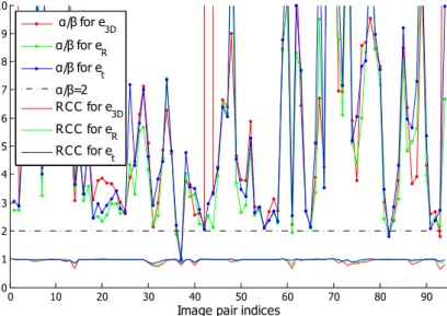
0 10 20 30 40 50 60 70 80 90 0 1 2 3 4 5 6 7 8 9 10
Image pair indices α/β for e3D α/β for eR α/β for et α/β=2 RC C for e3D RC C for eR RC C for et
Fig. 1. Dotted curves: estimated α/β for different image pairs (the order is irrelevant). Plain curves: regression correlation coefficient between eR, et, or e3D, and σ2Dα/N
β
when N is fixed (but not the configuration), with some slope −β also depend-ing on the image pair. It is confirmed by computdepend-ing the regression correlation coefficient (RCC) of e3D, eR, etwith σ2Dα/Nβ, which is in general very close to 1,
as can be seen in Figure 1 (bottom 3 curves, plotted on the same diagram). Besides, we also found empirically that σ2Dis more or less proportional to eF,
not only to the exact epipolar error. We thus hypothesize the relation:
eR, et, e3D∝
σ2Dα Nβ ∝
eFα
Nβ (3)
With a fixed distribution of points, we should have α = 1 for small errors. Still with a fixed configuration, but duplicating all matches, the covariance matrix of estimated parameters is halved; we should thus have β = 0.5. This is consistent with equation (1). However, it does not hold when point configuration varies. Experimentally, α and β can vary significantly depending on images pairs and match sampling. In our semi-synthetic dataset, β varies between 0.2 and 1.5. Yet, assuming relation (3), knowing α/β is sufficient to compare errors for a given image pair:
eFα Nβ < eF0 α N0 β ⇔ eFα/β N < eF0 α/β N0 (4)
The situation where all matched points are treated as inliners and contribute to estimating F amounts to preferring the largest N (smallest 1/N ) indepen-dently of eF, i.e., to α/β = 0. On the contrary, the larger α/β, the more
aggres-sively low-accuracy features should be discarded. As can be seen in Figure 1, α/β ≥ 2 almost consistently. (5)
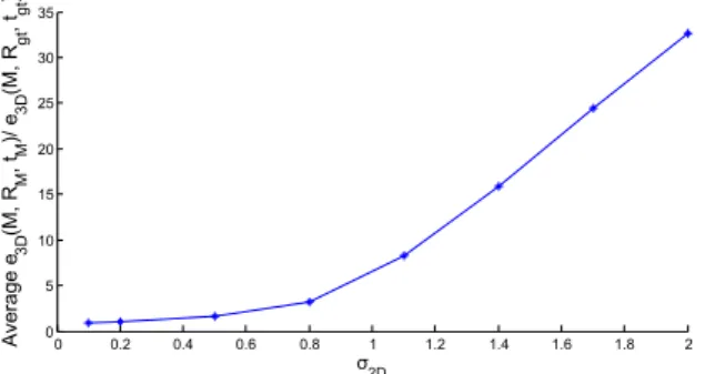
0 0.2 0.4 0.6 0.8 1 1.2 1.4 1.6 1.8 2 0 5 10 15 20 25 30 35 Average e 3D (M, R M , tM )/ e 3D (M, R gt , tgt ) σ2D
Fig. 2. Amplification of 3D reconstruction error when σ2Dgrows
Figure 2 compares the accuracy of reconstructing 3D points from noisy image points with ground-truth Rgt, tgtvs estimated RM, tM (average on image pairs).
The bigger σ2D, the more calibration errors amplify reconstruction errors.
3
Match Selection to Improve Accuracy
To improve accuracy, we estimate SfM using a selected subset of good matches. Cleaning up input matches. Although we use IRLS for estimating F , the level of accuracy we target may be sensitive to outliers remaining after RANSAC. We thus try to eliminate outliers from the set of input matches. We have to do it without introducing the bias of an early approximate calibration estimation, which would be the case if we were to first filter the matches using RANSAC. For this reason, we first clean up the matches using the K-VLD method [15]. Based on semi-local geometric and photometric consistency, it eliminates many outliers without any calibration assumption. Running ORSA afterwards on the resulting set of matches M typically only removes on the order of 10% of matches with a found threshold of less than 2-pixel error for estimating F .
Comparing subsets of matches. The SfM errors we want to reduce are eR(M ), et(M ), e3D(M ). But what can be easily measured given a pair of images
and a set of matches M is just eF(M ). However, as indicated by Eq. (3) and (4),
eR(M ), et(M ), e3D(M ) vary monotonically with eF(M )α/β/|M |. The basic idea
of match selection is to use only a subset of matches Msub⊂ M as soon as:
eF(Msub)α/β
|Msub|
< eF(M )
α/β
|M | (6)
However, α/β is a priori unknown for an arbitrary image pair. Moreover, we want to improve SfM without taking the risk to degrade it. What we need is a sufficient condition that reducing the number of matches will probably improve accuracy but most certainly will not reduce it. For this, we look for a possible value γ ≥ 0 such that, for any image pair, any set of matches M with corresponding α, β parameters, and any subset of matches Msub⊂ M ,
eF(Msub)γ |Msub| <eF(M ) γ |M | ⇒ eF(Msub)α/β |Msub| < eF(M ) α/β |M | (7)
We can then choose this optimal subset of matches Msub∗ for estimating F : Msub∗ = arg min
Msub⊂M
eF(Msub)γ
|Msub|
(8) The fundamental FM∗
sub minimizes reprojection errors w.r.t. ground truth Fgt.
Noting that (eF(Msub)/eF(M ))γ < |Msub|/|M | < 1 and hypothesizing (5),
we can choose γ = 2 because then (eF(Msub)/eF(M ))α/β < (eF(Msub)/eF(M ))γ,
ensuring condition (7). Parameter γ is chosen as a safe empirical lower bound, not an average value, which is more robust. Still, a general method to treat a specific class of images would be to run experiments as in Section 2.2 and pick a value γ ≤ α/β. Without loss of generally, we assume γ = 2 in the following. Exploring subsets of matches. The difficulty to find Msub∗ is to explore Msub⊂ M , as there are too many such subsets (2|M |). We propose to evaluate
just a fraction of them, that has the most chances to lead to smaller ratios eF(Msub)2/|Msub|. For this, we rank the matches in M and use this ordering to
explore only subsets of top-rank matches. More precisely, we look for a ranking function φ : M → R to order the matches into a sequence (mi)1≤i≤|M | such that
i < j ⇒ φ(mi) < φ(mj), and consider Msub(N ) = {mi | 1 ≤ i ≤ N }. If the
ranking function φ is highly correlated to the reprojection errors e2D(M, m),
and hence to the epipolar errors eF(M, m), then
min Msub⊂M eF(Msub)2 |Msub| = min N ≤|M | 1 N Msubmin⊂M |Msub|=N eF(Msub)2 ≈ min N ≤|M | 1 N eF(Msub(N )) 2 (9)
We may thus resort to:
N∗= arg min
N ≤|M |
eF(Msub(N ))2
N (10)
M∗= Msub(N∗) (11)
The number of subsets to explore is then reduced from 2|M |to |M |, which is still a lot given that M generally contains a few thousands of matches. Note that eF(Msub(N ))2/N is not necessarily convex. However, it is in practice “smooth”
enough for a reduced exploration of 8 ≤ N ≤ |M | to make sense. In our various experiments, we found it robust and accurate enough to ensure a minimum of 40% of matches in Msub(N ) and to explore fractions of M with a 5% step, i.e.,
to consider N = r|M | with ratio r = 0.4 + 0.05k and k = 0, . . . , 12.
Ranking matches. The choice of a ranking function φ varies with the kind of feature. For SIFT, it seems natural to consider the distance between fea-ture descriptors d(desc(x), desc(x0)) as an indicator of feature accuracy. Besides, Tang [25] showed that SIFT subsampling amplifies location error by the feature scale factor scale(x). This leads us to define the following ranking function:
Feature matching KVLD filter Match refinement Match ordering Subset Subset Subset Subset Model selection Images Accurate model
Fig. 3. A global view of our algorithm
Large features thus tend to be ordered last, unless their descriptors match well. Still, although they have a poor accuracy, they are often useful for robustness, which could be a issue if too many of them are discarded. But our use of K-VLD [15] provides enough (if not better) robustness improvement to compensate. On semi-synthetic data, made with first images from Mikolajczyk et al.’s dataset [18] and after applying an known homography, we found a correlation coefficient of 0.42 between φ and σ2D, which proves the relevance of φ for
or-dering M . It outperforms other indicators, such as feature saliency that has a correlation score of 0.02. The Lowe score (ratio of descriptor distance to next best match) has an individual correlation of 0.2, but it does not improve the global correlation when combined with φ.
Note that the definition of φ relies only on detection scale and on the SIFT descriptor, not on the detector. It can thus be used, e.g., for all detectors of Mikolajczyk et al. [18], including SURF, Harris-Affine and MSER. Transposition to other descriptors is direct, but the correlation coefficient should be checked. Algorithm. Our match selection algorithm is summarized on Figure 3. After feature detection and matching, matches M are cleaned up using K-VLD and ordered using the ranking function φ. Subsets Msub of sorted matches are
ex-plored to minimize eF(Msub)γ/|Msub| and the subset with the lowest value if
used to construct the estimated model.
Comparison to related methods. The PROSAC variant of RANSAC also constructs a series of match subsets and iterates first on better ones [7]. However, the target is not accuracy but fast convergence; robustness and precision are similar to RANSAC. Note that our method is not an alternative to RANSAC nor a fundamental matrix estimator, but a complement: a RANSAC variant as well as a fundamental matrix estimator are still needed to compute the calibration and the corresponding epipolar error eFfor the different Msubsubsets considered.
As a matter of fact, Section 5 shows that our method, combined with different variants of RANSAC, consistently provides much better results.
4
Least Square Focused Matching
We now present an extension of least squares matching (LSM) [10, 22] to bet-ter adjust the location of matching features. LSM is based on the hypothesis
that, locally, the region around the feature center is mostly planar, so that two matching regions are approximately related by homography, which in turn can be approximated by an affinity if the change of viewpoint is moderate. Besides, image intensity is also considered to possibly vary with an affine transformation. Finding the affine parameters (both geometric and radiometric) that best map the two regions provides a good estimate of point displacement. This is a non-linear adjustment problem. It can be addressed by an iterative scheme based on a first-order Taylor expansion expressing optical flow constraints: differenti-ating the affine relation between the two regions, a small change in the affine parameters can be related to a small change in the dissimilarity measure of the regions, to be minimized. Yet, contrary to ordinary optical flow [3], LSM is not restricted to small light changes, small rotation angles and small baselines.
With LSFM, we propose two improvements. First, instead of using a regular sampling grid around the features, we use an irregular grid focused on the center of the region to match. Second, we combine it with an image scale traversal to make it more robust to local minima. (We also tried estimating a homography rather than just an affinity, but it did not produce substantial improvements.)
Note that feature detection covariance [4, 12, 24, 29] is irrelevant here. What we do is, given a position p in I for which we know a roughly corresponding position p0 in I0, adjust p0 so that the regions around p in I and p0 in I0 corre-late better, under some geometric and photometric affinity to estimate. Feature points that match just happen to provide good initial correspondences for the refinement process. This is also widely different from refining the location of features detected as salient [16, 18]. Moreover, refining given matches leads to a better accuracy than refining detections before matching.
Initialization. Given two matching features, we measure the dissimilarity η between the region with the lowest scale s and the region with the highest scale s0 after enlarging by a factor of s0/s the sampling grid. We also rotate the grid according to the difference of orientation between the features. This initializes the affinity parameters in the iteration process.
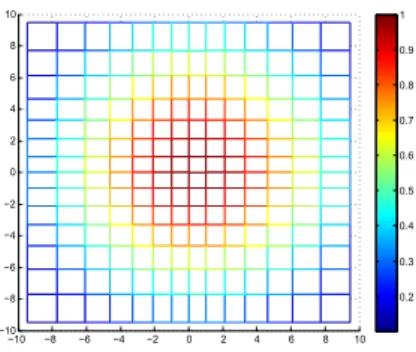
Focused grid. The image dissimilarity measure η in LSM is traditionally based on a regular sampling grid centered on interest points. This assumes a uniform transformation of the whole patches, which is true locally and slowly breaks down when moving away from the center. For this reason, we propose to use a grid focused on the patch center, i.e., denser in the center than in the border, which is additionally weighted by a Gaussian kernel to further concentrate on the center. Concretely, we use a grid whose lines are defined by a geometric progression: its coordinates are (u, v) = (sign(i)ρ|i|ρ−1−1, sign(j)ρ|j|ρ−1−1) for i, j ∈ {−n, . . . , n}. A standard Gaussian weight of 2πσ12exp(−
u2+v2
2σ2 ) is used on grid nodes (u, v).
Figure 4 illustrates the shape of our grid, with color representing the Gaussian weight. In experiments, we use a spline interpretation of order 5 to get subpixel intensity in a focused grid with n = 7, σ = 0.9 n and ρ = 1.1: samples at the grid border are then almost twice as dense (in one direction) as at the center.
−10 −8 −6 −4 −2 0 2 4 6 8 10 −10 −8 −6 −4 −2 0 2 4 6 8 10 0.2 0.3 0.4 0.5 0.6 0.7 0.8 0.9 1
Fig. 4. Focused grid: denser and heavier center (colors represent the Gaussian weight)
Scale exploration. Additionally, rather than directly adjusting the feature positions at their original scale, we perform a coarse-to-fine refinement. We start adjusting point location at a higher scale and progressively refine the location by reducing the scale until we reach the original scale. (An optimal scale is not search as in [14]: the original scale is best for accuracy.) It improves robustness, preventing some refinements to be caught in local minima. For this, we create a pyramid of images similar to the one used in SIFT detection. After convergence of the geometric and photometric parameters at a given scale, we restart with the corresponding location and parameters at the scale below. As a high blur may also cause deviation from the optimal solution, we make sure there is an actual improvement: if the measure of dissimilarity computed with the estimated parameters at the current scale is less than the dissimilarity on the lower scale using just feature scale and orientation, the latter is kept as initial parameters for the refinement at the lower scale. In our experiments, we explore 5 octaves of scale, dividing each octave in 2, i.e., with a geometric progression of ratio√2. Impact of the feature detector. SSD-based refinement is more accurate for regions with high gradients. SIFT does not necessarily detect points in such regions, but its robustness compensates. Besides it tends to find points within objects, where relative intensity is more stable, compared to corners that have strong but less stable gradients because they often correspond to occlusion edges. Match selection with match refinement. Match selection and match refine-ment are independent improverefine-ments that can be combined, match refinerefine-ment coming first (see Fig. 3). However, match refinement changes the correlation be-tween the match errors and the indicators of feature accuracy. When combined, the match ranking to create subset candidates (cf. Section 3) has to be changed. Based on experiments with the same semi-synthetic data as in Section 3, we found that, after match refinement, the dissimilarity measure η using the focused grid has correlates with the actual feature localization error, with score of 0.27. Besides, intuitively, the scaling and shearing of the image, as defined by the affinity estimate A, also has an impact on the quality of matching. Given orthogonal vectors (u, v) in I, we consider the value maxu,v|u
TATAv|
|Au||Av| , which is
simply expressed as χ = |λ1−λ2|
λ1+λ2 , where λ1, λ2> 0 are the eigenvalues of A
TA. It
has a correlation score of 0.12 with the localization error. By a linear regression over the same semi-synthetic data, we empirically define φ(m) = 0.3 η + 42.6 χ, which has a correlation of 0.34 with the location error. Note that feature scales no longer correlate with the location error (correlation is only 0.01) and are thus discarded from the ranking function.
5
Experiments
To evaluate our method, we consider some RANSAC variants among those that are considered the most suited for accuracy (as opposed, e.g., to robustness or speed) [6, 27]: RANSAC with iterative re-weighted least squares (IRLS) for fi-nal model estimation [27, method S1], RANSAC with M-estimator (MSAC), LO-RANSAC [8], MLESAC [26], and ORSA with IRLS [19]. IRLS tries to min-imize the sum of squares of geometric error between points in the right image and the epipolar line of corresponding points in left image. For each of these variants, we compare 4 settings: RANSAC alone, RANSAC preceded by match selection (MS), RANSAC preceded by match refinement (MR) using LSFM, and RANSAC preceded both by match refinement and match selection (MR+MS). A uniform threshold of 3 pixels (distance to epipolar line) is used in the RANSAC variants for outlier rejection, apart from ORSA that chooses the threshold au-tomatically. All the results we provide are averaged over 20 runs.
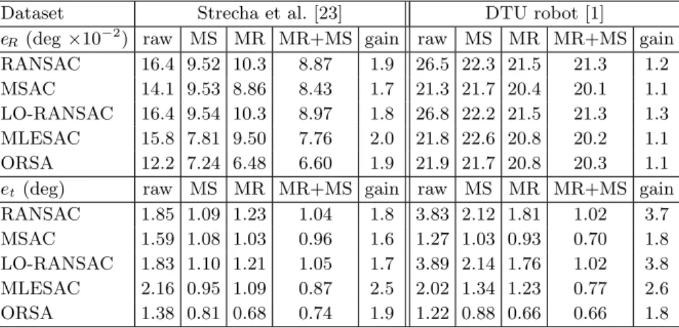
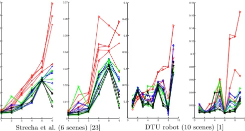
Only datasets with highly accurate ground-truth calibration can be used for validation. We experimented with the full dataset of Strecha et al. [23], a de facto standard in camera calibration: 6 groups of 8 to 30 images totaling 95 pairs of successive images. For each pair, SIFT feature points are detected and matched with the usual setting [16] (no tweaking as in Sect. 2.2), i.e., a descriptor distance ratio to next best match at most 0.8. We ran the same experiment with the DTU robot dataset [1]. However, as it is huge (about 0.5 To), we only considered 9 of the 60 groups of images, covering various themes (scenes 1, 2, 4, 9, 10, 12, 21, 28, 52), in the reduced format (fewer images, yielding 12 images pairs: 1-12, 12-24, 24-25, 25-26, 26-37, 37-49, 50-57, 57-64, 57-65, 57-94, 64-95, 64-119), with identical illumination condition (number 08 for all tests), but full-size images. Match selection and refinement. Figure 5 shows the average rotation and translation errors eR, etfor each scene of each dataset. Table 1 shows the average
results, illustrating both the separate and combined benefits of MS and MR. Gain factors attain 2.0 for rotation and 3.8 for translation. Note that most parameters are learned on other, widely different images [18]; only the lower bound γ = 2 is defined from feature distribution in [23] and nothing else. Our excellent results on [1, 23] suggests that these parameters make sense for a wide range of images. Focused matching. We compare our focused matching (LSFM, Section 4) with standard least square matching (LSM). Rather than considering planar scenes and measuring reprojection errors, we directly measure eR and et using
Table 1. Average rotation and translation errors: RANSAC alone (raw), + match selection (MS), + match refinement (MR), + both (MR+MS), and gain raw/(MR+MS)
Dataset Strecha et al. [23] DTU robot [1]
eR(deg ×10−2) raw MS MR MR+MS gain raw MS MR MR+MS gain
RANSAC 16.4 9.52 10.3 8.87 1.9 26.5 22.3 21.5 21.3 1.2 MSAC 14.1 9.53 8.86 8.43 1.7 21.3 21.7 20.4 20.1 1.1 LO-RANSAC 16.4 9.54 10.3 8.97 1.8 26.8 22.2 21.5 21.3 1.3 MLESAC 15.8 7.81 9.50 7.76 2.0 21.8 22.6 20.8 20.2 1.1 ORSA 12.2 7.24 6.48 6.60 1.9 21.9 21.7 20.8 20.3 1.1 et(deg) raw MS MR MR+MS gain raw MS MR MR+MS gain
RANSAC 1.85 1.09 1.23 1.04 1.8 3.83 2.12 1.81 1.02 3.7 MSAC 1.59 1.08 1.03 0.96 1.6 1.27 1.03 0.93 0.70 1.8 LO-RANSAC 1.83 1.10 1.21 1.05 1.7 3.89 2.14 1.76 1.02 3.8 MLESAC 2.16 0.95 1.09 0.87 2.5 2.02 1.34 1.23 0.77 2.6 ORSA 1.38 0.81 0.68 0.74 1.9 1.22 0.88 0.66 0.66 1.8
Table 2. Match refinement evaluation using LSM, LSM with focused grid, LSM with focused grid and scale exploration (LSFM), gain as improvement of LSFM over LSM
eR (deg ×10−2) LSM LSM + foc. grid LSFM gain
Strecha et al. [23] 7.55 6.73 6.48 1.17 DTU robot [1] 20.97 21.22 20.79 1.01 et (deg) LSM LSM + foc. grid LSFM gain
Strecha et al. [23] 0.84 0.72 0.68 1.25 DTU robot [1] 0.77 0.71 0.66 1.16
methods: LSM, LSM with focused grid, and LSM with focused grid and scale exploration (LSFM). We estimate errors after calibrating with ORSA+IRLS, which has the best performance in the above tests (see Table 1). Table 2 shows that, apart from a poor reduction of rotation error in the DTU robot dataset, the LSFM factor gain is 1.16 to 1.25.
6
Conclusion
In this paper we have studied, in the two-view case, the “quality vs. quantity” balance of point matches for structure from motion — a poorly addressed issue in the literature. We have found a correlation between SfM errors and a function of the number of matches and their epipolar errors. Using this relation, we have presented a new method for selecting relevant subsets of points to improve SfM accuracy. We have also proposed an improvement of an existing method to refine match locations. Using extensive experiments involving real data with ground-truth calibration, we have shown that match selection and match refinement independently lead to a major reduction of SfM errors over the best methods
1 2 3 4 5 6 0 0.05 0.1 0.15 0.2 0.25 0.3 0.35 0.4 0.45 1 2 3 4 5 6 0 0.01 0.02 0.03 0.04 0.05 0.06 0.07
Strecha et al. (6 scenes) [23]
0 2 4 6 8 10 0.2 0.25 0.3 0.35 0.4 0.45 0.5 0 2 4 6 8 10 0 0.02 0.04 0.06 0.08 0.1 0.12 0.14 0.16 0.18
DTU robot (10 scenes) [1]
Fig. 5. Average results on the datasets. Left: rotation error eR. Right: translation
error et. Colorred: raw RANSAC;blue: with match selection (MS);green: with match
refinement using LSFM (MR); black: with both match selection and match refinement (MR+MS). Line symbol -.-: RANSAC with IRLS; -*-: MSAC; -x-: LO-RANSAC; -o-: MLESAC; -/-: ORSA. Scenes are reordered by increasing rotation error of RANSAC
targeted at accuracy. Combining both methods, the error is reduced by factors up to 2.0 for rotations and 3.8 for translations, which is an enormous improvement. Our work is valuable for stereovision. Extending it to the multi-view case is not trivial because of track consistency. First, removing one match does not necessarily remove the associated points from the track and leads to a substan-tially different bundle adjustment problem. Second, the location of points in a track would need to be optimized simultaneously in all associated images. We actually want track selection (or reduction) as well as track refinement. Besides, a good term to minimize to assess the benefit of match reduction is likely to be linked to the total reprojection error with respect to all 3D points after bundle adjustment. A study similar to that of Section 2 thus has to be carried out.
Still, a lower bound of the possible improvement can be obtained by applying match selection (MS) on each image pair in an SfM pipeline, before actual pro-cessing by the system. A preliminary experiment on Strecha et al.’s dataset us-ing OpenMVG [21], a competitor to Bundler, shows improvements up to 15% on the average camera location error, in particular on scenes with wider viewpoint changes and less images (HerzJesu-P8 vs -P25, Castle-P19 vs -P30). Conversely, it may be the case that bundle adjustment is doing a good job at averaging on long tracks, compensating for the inaccuracy of point location. Track selection and track refinement are thus likely to be more profitable on difficult scenes.
Finally, most of our results are constructed on empirical studies. We however believe the “quality vs. quantity” issue deserves a better theoretical treatment, including a study of the influence of the configuration of points in images. Acknowledgements. This work was carried out in IMAGINE, a research pro-ject between ENPC and CSTB. It was partly supported by ANR propro-ject Stereo.
References
1. Aanæs, H., Dahl, A.L., Pedersen, K.S.: Interesting interest points. International Journal of Computer Vision 97(1), 18–35 (2012)
2. Baatz, G., K¨oser, K., Chen, D., Grzeszczuk, R., Pollefeys, M.: Leveraging 3D city models for rotation invariant place-of-interest recognition. IJCV 96(3), 315–334 (2012), http://dx.doi.org/10.1007/s11263-011-0458-7
3. Baker, S., Scharstein, D., Lewis, J., Roth, S., Black, M.J., Szeliski, R.: A database and evaluation methodology for optical flow. IJCV 92(1), 1–31 (2011)
4. Brooks, M.J., Chojnacki, W., Gawley, D., Van Den Hengel, A.: What value co-variance information in estimating vision parameters? In: Proceedings of the 8th IEEE International Conference on Computer Vision (ICCV). vol. 1, pp. 302–308. IEEE (2001)
5. Cao, Y., McDonald, J.: Viewpoint invariant features from single images using 3D geometry. In: WACV (2009)
6. Choi, S., Kim, T., Yu, W.: Performance evaluation of RANSAC family. In: BMVC. pp. 1–12 (2009)
7. Chum, O., Matas, J.: Matching with PROSAC – progressive sample consensus. In: CVPR (2005)
8. Chum, O., Matas, J., Obdrzalek, S.: Enhancing RANSAC by generalized model optimization. In: ACCV (2004)
9. Fischler, M.A., Bolles, R.C.: Random sample consensus: a paradigm for model fitting with applications to image analysis and automated cartography. CACM 24(6) (1981)
10. Gruen, A.: Adaptive least squares correlation: a powerful image matching tech-nique. S. Afr. J. of Photogrammetry, Remote Sensing and Cartography 14(3) (1985) 11. Hartley, R.I., Zisserman, A.: Multiple View Geometry in Computer Vision.
Cam-bridge University Press (2004)
12. Kanazawa, Y., Kanatani, K.: Do we really have to consider covariance matrices for image features? In: Proceedings of the 8th IEEE International Conference on Computer Vision (ICCV). vol. 2, pp. 301–306. IEEE (2001)
13. K¨oser, K., Koch, R.: Perspectively invariant normal features. In: ICCV (2007) 14. K¨oser, K., Koch, R.: Exploiting uncertainty propagation in gradient-based image
registration. In: BMVC (2008)
15. Liu, Z., Marlet, R.: Virtual line descriptor and semi-local graph matching method for reliable feature correspondence. In: BMVC (2012)
16. Lowe, D.: Distinctive image features from scale-invariant keypoints. IJCV 60(2), 91–110 (2004)
17. Matas, J., Chum, O., Urban, M., Pajdla, T.: Robust wide-baseline stereo from maximally stable extremal regions. Image and Vision Computing 22(10), 761–767 (2004)
18. Mikolajczyk, K., Schmid, C.: Scale & affine invariant interest point detectors. IJCV 60(1), 63–86 (2004)
19. Moisan, L., Stival, B.: A probabilistic criterion to detect rigid point matches be-tween two images and estimate the fundamental matrix. IJCV 57(3), 201–218 (2004)
20. Morel, J.M., Yu, G.: ASIFT: A new framework for fully affine invariant image comparison. SIAM Journal on Imaging Sciences 2(2), 438–469 (2009)
21. Moulon, P., Monasse, P., Marlet, R.: Adaptive Structure from Motion with a con-trario model estimation. In: ACCV (2012)
22. Pot˚uˇckov´a, M.: Image matching and its applications in photogrammetry. Ph.D. thesis, Aalborg Universitet (2004)
23. Strecha, C., von Hansen, W., Van Gool, L., Fua, P., Thoennessen, U.: On bench-marking camera calibration and multi-view stereo for high resolution imagery. In: CVPR (2008)
24. Sur, F., Noury, N., Berger, M.O.: Computing the uncertainty of the 8 point algo-rithm for fundamental matrix estimation. In: Proceedings of 19th British Machine Vision Conference (BMVC). pp. 96.1–96.10 (2008)
25. Tang, Z.: High precision in Camera calibration. Ph.D. thesis, ENS Cachan (2012) 26. Torr, P.H.S., Zisserman, A.: MLESAC: a new robust estimator with application to
estimating image geometry. CVIU 78(1), 138–156 (2000)
27. Torr, P.H., Murray, D.W.: The development and comparison of robust methods for estimating the fundamental matrix. IJCV 24(3), 271–300 (1997)
28. Wu, C., Clipp, B., Li, X., Frahm, J.M., Pollefeys, M.: 3D model matching with viewpoint-invariant patches (VIP). In: CVPR (2008)
29. Zeisl, B., Georgel, P.F., Schweiger, F., Steinbach, E.G., Navab, N., Munich, G.: Es-timation of location uncertainty for scale invariant features points. In: Proceedings of 20th British Machine Vision Conference (BMVC). pp. 1–12 (2009)