HAL Id: hal-01534795
https://hal.archives-ouvertes.fr/hal-01534795
Submitted on 8 Jun 2017
HAL is a multi-disciplinary open access
archive for the deposit and dissemination of
sci-entific research documents, whether they are
pub-lished or not. The documents may come from
teaching and research institutions in France or
abroad, or from public or private research centers.
L’archive ouverte pluridisciplinaire HAL, est
destinée au dépôt et à la diffusion de documents
scientifiques de niveau recherche, publiés ou non,
émanant des établissements d’enseignement et de
recherche français ou étrangers, des laboratoires
publics ou privés.
Using Empirically Validated Simulations to Control
802.11 Access Point Density
Tanguy Kerdoncuff, Alberto Blanc, Nicolas Montavont
To cite this version:
Tanguy Kerdoncuff, Alberto Blanc, Nicolas Montavont. Using Empirically Validated Simulations to
Control 802.11 Access Point Density. WCNC 2017 : IEEE Wireless Communications and Networking
Conference, Mar 2017, San Francisco, United States. pp.1 - 6, �10.1109/WCNC.2017.7925888�.
�hal-01534795�
Using Empirically Validated Simulations to Control
802.11 Access Point Density
Tanguy Kerdoncuff, Alberto Blanc, Nicolas Montavont
Telecom Bretagne/IRISA, Rennes, France
email: {firstname.lastname}@telecom-bretagne.eu
Abstract—Simulations are an essential tool for studying wire-less networks, yet great care must be taken when choosing the simulation parameters, in order to have results reflecting what would happen in a real network. Thanks to extensive traces containing scan results collected by pedestrian users in an urban setting, we select the parameters of different NS-3 modules so that the results obtained match what we observed in a real setting, contrary to what happens if one uses the default values of these modules. We extend the NS-3 simulator in order to faithfully simulate the scanning phase and in order to dynamically change the IP address assigned to Mobile Stations. Finally, we use the simulation parameters that have produced realistic results to analyze what happens when the Access Point density changes.
I. INTRODUCTION
One of the challenges faced by researchers when proposing new architectures or new protocols for wireless networks is that ideas that look good on paper do not always live up to expectations when they are implemented in the real world. Scalability issues, signal propagation characteristics or non representative topologies may significantly mitigate the performance of the newly proposed mechanisms. This is one of the reasons for which, over the last few years, a lot of efforts have been made to implement the proposed solution in real networks. Such a solution does indeed have several advantages but it comes at a significant cost in terms of time and effort. And it does have at least one non-negligible shortcoming: in a real network not all parameters can be easily changed, especially if some of the devices used are part of a production network. In other words, the relevance of using a real network with real traffic comes at the expense of not being able to change certain parameters.
WiFi is one technology that has proven its success over the years, with a growing number of Access Point (AP) being deployed around the globe. A significant number are in private homes, where they provide connectivity to the household members but, especially in dense urban environments, they can also be shared to offer Internet access to other customers of the same network provider, or to customers who have signed up for specific services, like those offered by FON.
Cellular network providers have shown a growing interest in using WiFi APs to offload some of the data traffic from their cellular networks. It is however hard to test new solutions (protocols and/or architectures) using a production network. Simulations can be an invaluable tool, as long as all the parameters are set correctly.
In this paper, we show how it is possible to use a simulator to reproduce the results obtained by collecting measurements in real WiFi networks, thanks to a WiFi war walking appli-cation called Wi2me [1]. This Android appliappli-cation runs on a smartphone and performs periodic scans to discover available APs. The data gathered by this application are then used to set up the network simulator with a representative Wi-Fi topology. APs are pseudo-randomly deployed inside buildings, and routes are drawn on virtual maps where a Mobile Station (MS) can move. We chose Network Simulator 3 (NS-3) as the simulation software, for its open source code and the variety of parameters in its module, and also because it is a very well known tool with a large active community behind it. With these tools, we are able to measure the impact of AP density, by varying the number of active APs. We can also study the network performance observed by a mobile client.
The remainder of the paper is organized as follows. In the next section, we discuss previous works on using real experi-ments to feed or verify network simulations. In Section III, we explain how we generate synthetic, yet representative, topologies and how we have modified Network Simulator 3 (NS-3). In Section IV, we present how we choose the simulation parameters, before using them to analyze changes in the AP density in Section V. Finally, Section VI concludes the paper.
II. RELATEDWORKS
Over the last several decades, many authors have worked on wireless channel models, resulting in a dauntingly vast literature on the subject (see for instance, the books by Tse and Viswanath [2], Rappaport [3], and Pedersen [4] and references therein). Such an abundance of different models has lead other authors to compare them, highlighting the non-negligible consequences on the result obtained by using different models (e.g., [5], [6]).
As pointed out by Kotz et al. [7], one should take care of avoiding common mistakes when simulating wireless net-works. Following this line of research, several works have compared simulation results with measurements from real wireless networks. Given the complexity of these models, which reflect the complexity of the real world, different authors have addressed different use cases and technologies. Some deal with sensor networks (e.g., [8], [9]), others with ve-hicular networks (e.g., [10], [11]), and yet others with 802.11
networks (e.g., [12]–[15]). To the best of our knowledge, only Yoo et al. [16] deal specifically with smart phones, studying how to best set the parameters in NS-3, all the other papers use laptops or different types of sensors.
The model and the parameter settings giving the most accurate simulation results depend on the type of device and on the environments. To the best of our knowledge, no previous work has validated simulation results using APs in an urban setting with smart phones as clients.
III. METHODOLOGYANDTOOLS
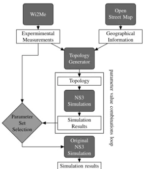
Fig. 1 shows how to use real world data to set the simulator parameters and create realistic topologies. The process consists in using experimental measurements and open street map information to generate topologies. Results obtained with a simulated MS moving within this topology help to configure the simulation parameters. The network simulator is then set to run original scenarios that would not be doable in a real topology.
A. Methodology
As previously mentioned, we have collected several traces (31 traces for 64km) by walking in the city center of Rennes (France), using the Wi2Me application [1]. This environment is characterized by fairly narrow streets (no large boulevards) and buildings of a few stories (between three and six) with businesses (stores, offices) as well as private residences. We take advantage of these traces in order to appropriately set the parameters of the NS-3 simulator.
Given that we do not know the actual location of the APs that were detected during the measurement campaigns, and given the limitations of the NS-3 simulator that force buildings to be rectangles, we generate random topologies. This has the added benefit of increasing the variability in the simulations by considering different, but equally representative and realistic topologies. Using the data provided by Open Street Map, we compute the distributions of a few key elements (see Section III-B below for more details) and generate synthetic topologies that have the same properties. We then randomly place APs inside buildings so that resulting AP density is the same that we have observed in the Wi2Me traces.
We simulate a user walking in the virtual topology, collect-ing the same measurements that we collected with Wi2Me, so that we can then compare the traces from the simulation to those collected with Wi2Me. In other words, we simulate what we have done in a real setting, in order to select the parameters of the simulation that best correspond to what we have empirically measured. Finally, we use these parameters to evaluate the performance of the AP-selection algorithm. As we cannot turn on and off real APs, we can only use simulations at this point.
B. Topology Generation
In this paper, we focus on pedestrians using MSs connected to WiFi networks in a dense urban environment. While users are walking in the streets, the overwhelming majority of APs
Simulation Results NS3 Simulation Topology Topology Generator Expermimental Measurements Geographical Information Wi2Me Open Street Map Parameter Set Selection Original NS3 Simulation Simulation results parameter v alue combinations loop
Fig. 1: Field testing and simulation data workflow
within range are located indoor. In order to simulate such a scenario, we need to produce a topology (streets and buildings) and then place the APs inside the buildings.
Thanks to Open Street Maps we computed the following features of the city center of Rennes, in order to produce random topologies with the same characteristics:
• the density of street corners • the density of building
• the distribution the streets’ lengths
• the distribution of the buildings’ wall lengths
• the distribution of the buildings’ distances to the streets We then randomly place APs inside buildings so that that resulting AP density is the same that we have observed in the Wi2Me traces.
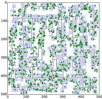
Figure 2 presents such an automatically generated topology. The black lines correspond to the streets where the MS can walk. The rectangles alongside them are the buildings, and the triangles represent the APs. As previously mentioned, buildings are rectangles due to an NS-3 limitation.
C. NS-3 Enhancements
NS-3 already comes with a rich WiFi implementation, including scanning, association to APs, traffic that takes into account the positions of the different transmitters. However the default implementation lacks a few key features needed in our use case. We implemented a Medium Access Control (MAC) layer inheriting from NS-3’s sta-wifi-mac. It features the ability to scan periodically even when already associated to an AP, store scan results, and to compare the candidate APs to the one it is currently using (if any). It also triggers handovers to the best possible candidate when the Receiving Signal Strength Information (RSSI) of the current AP drops below a threshold value, as an actual WiFi station would do. On top of these MAC layer handovers, we also implemented network
Fig. 2: Realistic topology generated for simulation
layer handovers, having the station pick up an appropriate IP address respecting its new AP’s Classless Inter-Domain Routing (CIDR) prefix.
IV. SELECTING THEBESTSIMULATIONPARAMETERS
As demonstrated by [6], the choice of a propagation model for an NS-3 experiment will dramatically impact the behaviour of the simulated nodes such as the traffic they will be able to transmit, or even their ability to communicate at all. One needs not only to choose a propagation model but also to decide the values of different parameters. While this flexibility allows to simulate almost any situation, finding an appropriate value for each parameter is a critical part of the simulation design. Because our work revolves around WiFi transmission, the modules we especially need to properly configure are the propagation model, and the WiFi physical layer. More precisely, these are the choices that we must make:
• Choice of the Propagation model: since our scenario includes buildings, our choices in terms of propagation models are limited to two candidates: OhBuildingsProp-agationLossModel and HybridBuildingsPropagationLoss-Model.
• Propagation model calibration: both aforementioned models have the following configuration parameters:
– The standard deviation of the shadowing for outdoor nodes.
– The standard deviation of the shadowing for indoor-outdoor transmissions.
– The additionnal loss caused by inner walls.
• Physical layer calibration: the WiFi physical layer includes these configuration parameters:
– The energy threshold over which a received signal can be detected by the physical layer.
– The energy threshold over which the medium is considered busy by the physical layer.
– The station’s transmission and reception gains. – The maximal and minimal transmission powers
available to the MS.
– The Noise figure corresponding to the station recep-tor’s imperfections.
We use the default values for the parameters of the AP modules, as these have already been thoroughly studied and can be considered trustworthy. On the contrary, parameters from the propagation models are intimately linked to the geographic environment and will vary from place to place. The MS’s physical layer’s parameters will also need to be chosen in order to properly model a smartphone, a different type of device from those modelled by the default parameters. A. Empirical Validation
Thanks to the Wi2Me traces, we can empirically verify the following metrics:
• The number of APs responding to a scanning request. • The average of all the RSSIs of the scanning responses
from each AP.
These metrics were chosen because both the RSSI at wich a MS receives messages from the AP, and its ability to see it at all will directly impact the simulations described in Section V. With the Wi2Me traces as a baseline, we simulate scanning campaigns in randomly generated topologies as explained in Section III-B. By varying the configuration parameters over a reasonably wide range, we determine which values best match the empirical traces. See the first column of Table III for a summary of the total simulation time and other metrics. B. Selected Parameter Values
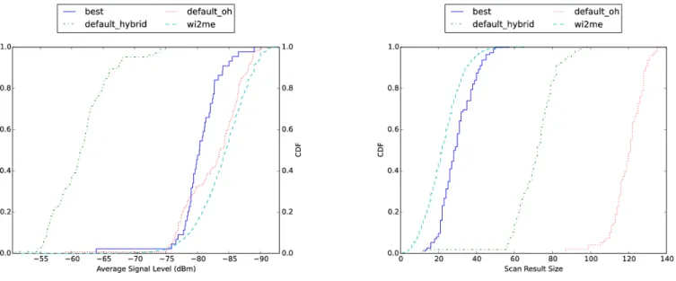
Figures 3a and 3b present the Cumulative Distribution Functions (CDFs) for both metrics, generated from field data as well as simulations using propagation models in their default configuration and simulations using a custom set of parameters values. Figure 3a presents the CDFs of the average RSSI value for each AP, and shows that the OhBuildingsPropagationLossModel with its default parameter values is already a pretty good fit for the field data baseline. For this reason, it will be preferred, in the rest of this work, to its counterpart, the HybridBuildingsPropagationLossModel. On the other hand, Figure 3b shows some non negligible differences in the number of APs that respond to a scanning request by the station. Our goal is therefore to find the values of the parameters that improve the accuracy of this metric, without disrupting an already decent representation of the APs’ power levels.
Table I shows the default values and the values that best match the Wi2Me traces. We have used the well-known the Kolmogorov Smirnov test [17] (D-Statistic) to measure the distance between two CDFs. As we are interested in matching two CDFs (the AP average RSSI and the Scan Result Size), we are faced with a multi-objective optimization problem, where each one of the eight columns of Table I corresponds to a
(a) Average signal strength of observed APs CDF (b) Number of APs responding to a scan CDF
Fig. 3: Comparison of metrics obtained through simulation and field testing TABLE I: Parameter Value Selection
Outdoor Nodes Shadowing std. dev. (dB) Indoor/Outdoor Transmission Shadowing std. dev. (dB) Internal Walls Loss (dBm) Energy Detec-tion threshold (dBm) CCA Busy energy threshold (dBm) Station Tx/Rx Gain (dBi) Station Transmission Power (dB) Receptor Noise Figure(dB) Parameter Range [2:16] [2:16] [2:16] [-100:-88] [-100:-96] [-1:8] [2:27 ] [4:16] NS-3 Defaults 7 5 5 -96 -99 1 16 7 Best Match 10 8 12 -92 -97 0 8 12
TABLE II: D Statistics between simulations and field data
Oh default Hybrid default best match
Scan Result Size 0.99 0.94 0.32
Average RSSI per AP 0.16 0.90 0.42 Average D Statistic 0.58 0.92 0.37
variable. Unsurprisingly, values that minimize one objective do not minimize the other, we therefore decided to choose values that minimized the average of both D-Statistics. Table II gives the value of the D-statistic for the default NS-3 settings as well as the best match. With our selection of simulation parameters, we manage a combined D-Statistic of 0.37 instead of the 0.58 and 0.92 values obtained with the default parameters. It is achieved through a much better fit for the scan result size, with a D statistic of 0.32 instead of values over 0.9 for the default, whithout degrading the D-Statistic for the average rsssi per AP.
While the range over which each parameter varied was purposely wide, we still end up with realistic parameter values. The interpretation of these values can be made along two axis:
the degradation of the MS’s performance, and the degrada-tion of the environment. Degrading the MS’s performance is legitimate, as we make the model evolve from representing a classical 802.11 client to a lightweight smartphone, with for example a 0 dBi antenna gain, as chosen by Yoo et al. [16]. Similarly, choosing values the correspond to a more hostile environment is not shocking, as there can be additional obstacles in the way of the transmission, for example internal walls or furniture affecting the Internal Wall Loss parameter. There can also be other factors, such as moving and static vehicles resulting in additional variations of the shadowing (Outdoor Nodes Shadowing parameter).
V. CONTROLLINGACCESSPOINTDENSITY
We have previously proposed an algorithm to select a subset of APs in order to cover a given area [18]. The idea being that, given the large number of available APs in dense urban environments, such as city centers, it is possible to save energy by switching some of them off, as long the overall coverage area does not change. Such a minimal set of APs could also be used by the MSs in order to select the best AP when performing a handover. Two main parameters are used to determine the way we pick a collection of APs based on scanning campaign results:
Best simulation pa-rameters selection Subset experiments Simulated time (h) 2142 3628 Distance traveled (km) 15334 25507 Scanning responses 4 402 665 7 983 162 Handovers 0 26703 Traffic (GB) 0 339.174
TABLE III: Summary of simulation characteristics
• Overlapping: The number of AP we try to have available at any position. This is required to let multiple users use the AP subset, but also to control the handover success rate.
• Minimal RSSI: This is the minimal RSSI of an AP’s
response to a scan in order to consider that said AP covers a specific position.
More details on the AP selection algorithm are available in [18], but the core concept is to select the smallest number of APs that provide the required overlapping coverage at every position of the topology. Using simulation was also the opportunity to vary these two parameters and see which fared the best. Trying for example to select APs based on their bare presence, with RSSIs down to -95 dBm, or based on their areas of best coverage around -55 dBm. This section will detail the properties and performance of two such AP subsets, compared to an hypothetic baseline: all the available APse on the map. Here are their details:
• Overlapping 2: Computed from simulated scanning campaigns, with a minimal RSSI of -65 and an overlap of 2
• Overlapping 4: Computed from simulated scanning campaigns, with a minimal RSSI of -65 and an overlap of 4
• Totality: The entire collection of APs available in the
area
We run simulations for each of these subsets, with a MS walking in our topology at the speed of two meters by second, selecting APs and generating traffic towards an application server reachable by all the APs. Table IV gives the number of APs present in these subsets, as well as the average throughput that the MS was able to achieve when associated. The second column of Table III shows the summary of some of the characteristics of these simulations.
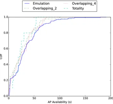
Figure 4 presents the CDF of the session duration, that is the time the MS was able use an AP (between the moment it associated to it to the last packet that it was able to transmit). It shows a reasonably similar session duration in each case. It is worth noting that running such an experiment on a production network is extremely hard, as it would require the cooperation of all the APs involved as they would need to offer IP connectivity to the MS, ideally by quickly assigning an IP address to the MS, without the delays imposed by commonly used captive portals.
Fig. 4: CDF Of Session Times for different AP Subset types
Subset AP Count Throughput on
Asso-ciation (kB/s)
Overlapping 2 16 54
Overlapping 4 32 117
Totality 875 108
TABLE IV: Count of Access Points in subsets
Another way to gather such data is emulation. Still based on the war walking campaings used to characterize our target en-vironment, we computed an actual AP subset for a geographic area in the city center. The Wi2Me android application used to perform said campaign also has an emulation mode to asses the viability of such an AP collection. It first behaves in the regular smartphone manner by scanning on all available channels and picking the best available AP member of the subset. While it cannot connect to a protected AP in order to generate traffic, Wi2Me is still able to send probe requests on the AP’s channel, in our case at the frequency of ten per second, and to monitor the response’s RSSI. Under a critical threshold, we consider no more traffic could have been generated. We are this way able to establish an emulated association time distribution for an AP subset, presented alongside the simulation results, in Figure 4. Based on the same geographic area used as the basis for our simulations, this emulation data presents a reasonably close behavior to the results of our simulations.
VI. CONCLUSION
In this paper, we presented a methodology combining simulation and field experimentation in order to study dense 802.11 WiFi deployment. We showed how a topology could be generated in order to represent a specific area. We also evaluated how well NS-3 was able to simulate said topology when compared to field data. While some metrics regarding
the power levels were satisfactory, some, more specific to our problematic such as the perception of the AP density, were not, and we showed how this could be improved. Through the presented use case of AP selection, we made use of our accurate simulation of the urban environment to evaluate different AP subsets, a study that could hardly have been real-ized as a real experimentation. This study opens perspectives around this collaboration of experimentation and simulation. The simulation parameter selection problem could definitely be improved by coupling its simulation and evaluation phases in a tighter manner. A genetic algorithm could for example run simulations for a given population of parameter values, evaluate its most promising members by comparing them to field data, mutate them and pass on the next generation. While human validation would probably remain needed at the end of the process, this fully integrated approach would make the process much more accurate. Another promising perspective is in the characterisation of a geographic area, both by topology generation, and by simulation parameter values. Wether they change from town to town, or if families that share the same characteristics can be identified would be both interesting and useful.
ACKNOWLEDGEMENTS
The authors would like to thank Christophe Couturier, Nicolas Kuhn and Tanguy Ropitault for advice and expertise on NS-3 and propagation Models.
Experiments presented in this paper were carried out using the Grid’5000 testbed, supported by a scientific interest group hosted by Inria and including CNRS, RENATER and several Universities as well as other organizations (see https://www. grid5000.fr).
This work has received a French government support granted to the CominLabs excellence laboratory and managed by the National Research Agency in the ”Investing for the Future” program under reference ANR-10-LABX-07-01
REFERENCES
[1] G. Castignani, A. Blanc, A. Lampropulos, and N. Mon-tavont, “Urban 802.11 community networks for mobile users: current deployments and prospectives,” Mobile networks and applications, vol. 17, no. 6, pp. 796–807, 2012.
[2] D. Tse and P. Viswanath, Fundamentals of wireless communication. Cambridge university press, 2005. [3] T. Rappaport, Wireless Communications: Principles and
Practice. Prentic Hall, 1996.
[4] G. F. Pedersen, COST 231-Digital mobile radio towards future generation systems. EU, 1999.
[5] A. Iyer, C. Rosenberg, and A. Karnik, “What is the right model for wireless channel interference?” IEEE Transactions on Wireless Communications, vol. 8, no. 5, pp. 2662–2671, 2009.
[6] M. Stoffers and G. Riley, “Comparing the ns-3 propa-gation models,” in 2012 IEEE 20th International Sym-posium on Modeling, Analysis and Simulation of Com-puter and Telecommunication Systems, 2012, pp. 61–67. [7] D. Kotz, C. Newport, R. S. Gray, J. Liu, Y. Yuan, and C. Elliott, “Experimental Evaluation of Wireless Simulation Assumptions,” in Proceedings of the 7th ACM International Symposium on Modeling, Analysis and Simulation of Wireless and Mobile Systems, 2004, pp. 78–82.
[8] S. Woo and H. Kim, “An Empirical Interference Modeling for Link Reliability Assessment in Wireless Networks,” IEEE/ACM Trans. Netw., vol. 21, no. 1, pp. 272–285, 2013. (visited on 10/05/2016).
[9] G. P. Halkes and K. G. Langendoen, “Experimental Evaluation of Simulation Abstractions for Wireless Sensor Network MAC Protocols,” EURASIP J. Wirel. Commun. Netw., vol. 2010, 24:1–24:2, 2010.
[10] C. Sommer, D. Eckhoff, R. German, and F. Dressler, “A computationally inexpensive empirical model of IEEE 802.11p radio shadowing in urban environments,” in WONS, 2011 Eighth International Conference, 2011, pp. 84–90.
[11] T. Mangel, O. Klemp, and H. Hartenstein, “A validated 5.9 GHz Non-Line-of-Sight path-loss and fading model for inter-vehicle communication,” in ITST, 2011 11th International Conference, 2011, pp. 75–80.
[12] K. Tan, D. Wu, A. Chan, and P. Mohapatra, “Comparing simulation tools and experimental testbeds for wireless mesh networks,” in WoWMoM, 2010 IEEE International Symposium, 2010, pp. 1–9.
[13] S. Ivanov, A. Herms, and G. Lukas, “Experimental Validation of the ns-2 Wireless Model using Simulation, Emulation, and Real Network,” in KiVS, 2007 ITG-GI Conference, 2007, pp. 1–12.
[14] R. Khattak, A. Chaltseva, L. Riliskis, U. Bodin, and E. Osipov, “Comparison of Wireless Network Simulators with Multihop Wireless Network Testbed in Corridor Environment,” en, in Wired/Wireless Internet Commu-nications, 6649, DOI: 10.1007/978-3-642-21560-5 7, 2011, pp. 80–91. (visited on 10/05/2016).
[15] M. Bredel and M. Bergner, “On the Accuracy of IEEE 802.11g Wireless LAN Simulations Using OMNeT++,” in Proceedings of the 2Nd International Conference on Simulation Tools and Techniques, 2009, 81:1–81:5. [16] S. Yoo, Y. Shin, S. Kim, and S. Choi, “Toward realistic
wifi simulation with smartphone physics,” in WoWMoM, 2014 IEEE 15th International Symposium, 2014, pp. 1– 6.
[17] F. J. Massey, “The kolmogorov-smirnov test for good-ness of fit,” Journal of the American Statistical Associ-ation, vol. 46, no. 253, pp. 68–78, 1951.
[18] D. Shehadeh, N. Montavont, T. Kerdoncuff, and A. Blanc, “Minimal access point set in urban area wifi net-works,” in WiOpt, 2015 13th International Symposium, IEEE, 2015, pp. 221–228.