HAL Id: hal-01467446
https://hal.archives-ouvertes.fr/hal-01467446
Submitted on 1 Oct 2018
HAL is a multi-disciplinary open access
archive for the deposit and dissemination of sci-entific research documents, whether they are pub-lished or not. The documents may come from teaching and research institutions in France or abroad, or from public or private research centers.
L’archive ouverte pluridisciplinaire HAL, est destinée au dépôt et à la diffusion de documents scientifiques de niveau recherche, publiés ou non, émanant des établissements d’enseignement et de recherche français ou étrangers, des laboratoires publics ou privés.
A revised Durbin-Wu-Hausman test for industrial robot
identification
Alexandre Janot, Pierre Olivier Vandanjon, Maxime Gautier
To cite this version:
Alexandre Janot, Pierre Olivier Vandanjon, Maxime Gautier. A revised Durbin-Wu-Hausman test
for industrial robot identification. Control Engineering Practice, Elsevier, 2016, 48, pp.52-62.
See discussions, stats, and author profiles for this publication at: https://www.researchgate.net/publication/289372634
A revised Durbin-Wu-Hausman test for industrial robot identification
Article in Control Engineering Practice · March 2016
DOI: 10.1016/j.conengprac.2015.12.017 CITATIONS 2 READS 127 3 authors:
Some of the authors of this publication are also working on these related projects: Distributed electric Propulsion for Small Business AircraftView project
Master/Engineering Project: Sensorless Vector Control of BLDC Motors for mini-dronesView project Alexandre Janot
The French Aerospace Lab ONERA
92PUBLICATIONS 406CITATIONS SEE PROFILE
Pierre Olivier Vandanjon
Institut Français des Sciences et Technologies des Transports, de l’Aménagement …
59PUBLICATIONS 338CITATIONS SEE PROFILE Maxime Gautier University of Nantes 187PUBLICATIONS 2,892CITATIONS SEE PROFILE
All content following this page was uploaded by Alexandre Janot on 04 March 2018.
A Revised Durbin-Wu-Hausman Test for Industrial
Robot Identification
Alexandre JANOT, Pierre-Olivier VANDANJON and Maxime GAUTIER
Alexandre Janot (Corresponding author), French Aerospace Lab, 2 Avenue Edouard Belin, BP 74025,
31055 Toulouse Cedex 4, France; Email: [email protected]
Pierre Olivier Vandanjon, French Institute of Science and Technology for Transport, Development and
Network (IFSTTAR), 44344 Bouguenais, France; Email: [email protected]
Maxime Gautier, University of Nantes and IRCCyN, 1, rue de la Noë - BP 92 101 - 44321 Nantes CEDEX
03, France ; Email: [email protected]
Abstract: This paper addresses the topic of robot identification. The usual identification method makes use of the inverse dynamic model (IDM) and the least squares (LS) technique while robot is tracking exciting trajectories. Assuming an appropriate bandpass filtering, good results can be obtained. However, the users are in doubt whether the columns of the observation matrix (the regressors) are uncorrelated (exogenous) or correlated (endogenous) with the error terms. The exogeneity condition is rarely verified in a formal way whereas it is a fundamental condition to obtain unbiased LS estimates. In Econometrics, the Durbin-Wu-Hausman test (DWH-test) is a formal statistic for investigating whether the regressors are exogenous or endogenous. However, the DWH-test cannot be straightforwardly used for robot identification because it is assumed that the set of instruments is valid. In this paper, a Revised DWH-test suitable for robot identification is proposed. The Revised DWH-test validates/invalidates the instruments chosen by the user and validates the exogeneity assumption through the calculation of the QR factorization of the augmented observation matrix combined with a F-test if required. The experimental results obtained with a 6 degree-of-freedom (DOF) industrial robot validate the proposed statistic.
Index Terms: Robots identification, Rigid robot dynamics, Instrumental variable method, Heteroskedasticity, DWH-test, Wald-statistic.
1
Introduction
The usual robot identification method makes use of the continuous-time inverse dynamic model and the least squares (LS) technique while the robot is tracking some exciting trajectories. This explains why robot identification belongs to the closed-loop identification of continuous-time models from sampled data. This method, called as Inverse Dynamic Identification Model with Least Squares method (IDIM-LS), has been successfully applied to identify the inertial parameters of several prototypes and industrial robots, (Olsen et al. 2002), (Swevers et al. 2007), (Hollerbach et al. 2008), (Calanca et al. 2011), (Gautier et al. 2013) and (Janot et al. 2014, a) among others. Good results are obtained provided that an appropriate bandpass filtering of the joint positions is used to calculate the joint velocities and accelerations. However, because robots are identified in closed loop, the users can doubt whether the columns of the observation matrix (the regressors) are correlated with the error terms (endogenous) or not (exogenous) even with a data filtering, see e.g. (Söderström and Stoica 1989), (Garnier and Wang 2008), (Young 2011) and (Gilson et al. 2011).
Other identification methods were tried: the Total Least-Squares (Xi 1995), the Set Membership Uncertainty (Ramdani and Poignet 2005), an algorithm based on Linear Matrix Inequality (LMI) tools (Indri et al. 2002), a maximum likelihood (ML) approach (Olsen et al. 2002), the Closed-Loop Output-Error method (Landau and Karimi 1997), (Landau 2001), (Östring et al 2003) and (Gautier et al. 2013), an algorithm based on neural network (Soewandito et al. 2011), a Bayesian approach (Ting et al. 2006), the extended Kalman filter (Gautier and Poignet 2001) and (Kostic et al. 2004), a method which estimates the nonlinear effects in the frequency domain (Wernholt and Gunnarsson 2008) and the Unscented Kalman Filter (Dellon and Matsuoka 2009). Although all these techniques are of interest, they do not really improve the IDIM-LS method combined with an appropriate data filtering. Furthermore, the robustness against data filtering was not studied, some of these approaches were not validated on a 6 degrees-of-freedom (DOF) industrial robot and the condition that the regressors are not correlated with the error terms is not addressed whereas it is a critical condition to obtain unbiased estimates (Hausman 1978), (Davidson and MacKinnon 1993) and (Wooldridge 2009). This condition is called as the exogeneity condition.
The Instrumental Variable method (IV) provides unbiased estimates while the regressors are endogenous (Söderström and Stoica 1989), (Garnier and Wang 2008) and (Young 2011). A generic IV method for industrial robots identification is proposed in (Janot et al. 2014, a) and (Janot et al. 2014, b). This approach called as the IDIM-IV method was successfully validated on a 2 DOF prototype robot and on a 6 DOF industrial robot. However, the validity of the instruments was not addressed and using the IV method while the regressors are exogenous provides inefficient unbiased estimates i.e. their variances are not minimal (Hausman 1978), (Davidson and MacKinnon 1993) and (Wooldridge 2009).
In Econometrics, the Durbin-Wu-Hausman test (DWH-test) is a formal statistic for investigating whether the regressors are exogenous or endogenous (Hausman 1978). The DWH-test makes use of the Two Stages Least Squares (2SLS) technique and an augmented LS regression. However, the DWH-test cannot be straightforwardly used for robot identification because it is implicitly assumed that the instrumental matrix is well correlated with the observation matrix and uncorrelated with the errors. Furthermore, the econometric models are empirical whereas the models used in mechanical engineering are based on physical laws (e.g. the Newton's laws).
In this paper, it is proposed to bridge the gap between Econometrics theory and Control engineering practice by presenting a Revised DWH-test suitable for identification of robots. This revisited statistic validates/invalidates the model chosen by the user and the exogeneity condition is validated by the QR factorization of the augmented observation matrix combined with the F-test.
A condensed version of this work has been presented in (Janot et al. 2013). This paper contains detailed proofs to enlighten the theoretical understanding of the Revised DWH-test, heteroskedasticity is taken into account and additional experimental results are provided.
The rest of the paper is organized as follows. Section 2 recalls the IDIM-LS method and reviews the theory of Econometrics. Section 3 introduces the Revised DWH-test while Section 4 is devoted to experimental results. Finally, Section 5 concludes the paper.
2
Theoretical Background: Modelling, identification of robots and
Introduction of the DWH-test
2.1
Modelling and identification of robots
The inverse dynamic model (IDM) of robot with n moving links calculates the
(
n×1)
joint torquesvector τidm as a function of generalized coordinates and their derivatives (Khalil and Dombre 2002),
( )
( )
,idm= +
τ M q qɺɺ N q qɺ , (1)
where q, qɺ and qɺɺ are respectively the
(
n×1)
vectors of generalized joint positions, velocities andaccelerations; M q
( )
is the(
n n×)
inertia matrix; N q q( )
,ɺ is the(
n×1)
vector of centrifugal, Coriolis, gravitational and friction torques.The modified Denavit and Hartenberg (MDH) notation allows to obtain an IDM which is linear in
relation to a set of base parameters β
(
, ,)
idm =
τ IDM q q qɺ ɺɺ β , (2)
where IDM q q q
(
, ,ɺ ɺɺ)
is the(
n b×)
matrix of basis functions of bodies dynamics and β is the(
b×1)
vector of base parameters.The base parameters are the minimum number of dynamic parameters from which the IDM can be calculated. They are obtained from the standard dynamic parameters by regrouping some of them
with linear relations (Mayeda et al. 1990). The standard parameters of a link j are XXj, XYj, XZj,
j
YY , YZj and ZZj the six components of the inertia matrix of link j at the origin of frame j; MXj,
j
MY and MZj the components of the first moment of link j; Mj the mass of link j; Iaj a total
inertia moment for rotor and gears of actuator j; Fvj and Fcj the viscous and Coulomb friction
parameters of joint j.
( )
= idm−( )
,M q qɺɺ τ N q qɺ . (3)
Proportional-Derivative (PD) and Proportional-Integral-Derivative (PID) controls are often
implemented to identify the dynamic parameters. The joint j signal control
j
vτ is given by
( )
(
)
j j rj mesj
vτ =C s q −q , (4)
where Cj
( )
s is the transfer function of the joint j controller,j
r
q is the joint j position reference,
j
mes
q is the measurement of qj the joint j position, s is the time derivative operator i.e. s=d dt/ .
The data available from robots controllers are qmes the
(
n×1)
vector of measurements of q and vτ ,the
(
n×1)
vector of control signals. The joint torques are connected with the control signals by thefollowing relation
τ τ
=
τ G v , (5)
where Gτ is the
(
n n×)
diagonal matrix of drive gains. The diagonal components of Gτ have a priorivalues given by manufacturers.
In (2), q is estimated with qˆ obtained by filtering qmes through a lowpass Butterworth filter in both
the forward and reverse directions.
( )
q qˆ ˆɺ ɺɺ, are calculated with a central differentiation algorithm of qˆ. τ being perturbed by high-frequency disturbances, a parallel decimation procedure is used to
eliminate torque ripples (see (Gautier et al. 2013) for the details).
Because of uncertainties, the
(
n×1)
vector of the actual joint torques τ differs from τidm by an errore. The model (2) is sampled while the robot is tracking trajectories (see (Gautier et al. 2013) for the
details). After data acquisition and data filtering, the following overdetermined linear system is obtained
( )
=(
ˆ , ,ˆ ˆ)
+y τ X q q q βɺ ɺɺ ε, (6)
where y τ
( )
is the( )
r×1 measurements vector built from the actual torques τ; X q q q(
ˆ , ,ˆ ˆɺ ɺɺ)
is the(
r b×)
observation matrix built from the sampling of IDM q q q(
ˆ , ,ˆ ˆɺ ɺɺ)
; ε is the( )
r×1 sampled vector ofe; r= ⋅n ne is the number of rows in (6), ne being the number of rows in a subsystem j.
Relation (6) is the Inverse Dynamic Identification Model (IDIM). The columns of X q q q
(
ˆ , ,ˆ ˆɺ ɺɺ)
are theregressors. ε is assumed to have zero mean, to be serially uncorrelated with a covariance matrix Ω
partitioned so that
(
2 2 2)
1 ne j ne n ne diag σ σ σ = Ω I ⋯ I ⋯ I , e nI being the
(
ne×ne)
identity matrix. 2j
σ
is estimated through the Ordinary Least Squares (OLS) solution of a subsystem j (see (Gautier et al.
2013) for the details). The IDIM-LS estimates and their covariance matrix are given by
(
)
1 1 1 ˆ T T LS − − − = β X Ω X X Ω y, ˆ(
T 1)
1 LS − − = Σ X Ω X . (7)The IDIM-LS estimates are unbiased if
( )
TE X ε =0, (8)
where E
( )
. is the expectation operator (Davidson and MacKinnon 1993).Because robots are identified in closed loop, the users can doubt whether X q q q
(
ˆ , ,ˆ ˆɺ ɺɺ)
is correlatedwith ε or not. To overcome the problem of a correlation between X and ε, the
Two-Stage-Least-Squares (2SLS) technique is an appropriate method.
2.2
Review of theory of Econometrics
The 2SLS method estimates β with two LS regressions. Researchers in Econometrics consider the
model (6) as the reduced form of the general model defined by
= + = + y Xβ ε X ZΠ V, (9)
where Z is the
(
r×z)
instrumental matrix with z≥b; Π is the(
z b×)
matrix of coefficients to beidentified and V is a
(
r b×)
matrix of error terms.The columns of Z are called instruments. If the following assumptions hold rank
( )
Z =b,( )
TE Z ε =0
,
( )
TE Z V =0 and E
( )
V =0, Z is said valid.The first stage calculates Πˆ , the LS estimate of Π, given by
( )
1ˆ = T − T
Π Z Z Z X. Xˆ , the projected of X
onto the space spanned by the columns of Z, is given by
( )
1 ˆ ˆ T T Z − = = = X ZΠ Z Z Z Z X P X, (10) where( )
T 1 T Z − =P Z Z Z Z is the idempotent
(
r r×)
projection matrix of Z.The second stage calculates the 2SLS estimates. Assuming that T ˆ ˆT
Z =
X P X X X is nonsingular i.e.
( )
ˆrank X =b, the 2SLS estimates and their associated covariance matrix are given by (Wooldridge
2009)
(
)
1 1 1 2 ˆ ˆT ˆ ˆT SLS − − − = β X Ω X X Ω y,(
1)
1 2 ˆ ˆT ˆ SLS − − = Σ X Ω X . (11)If z=b the 2SLS estimates collapse to the IV estimates given by ˆ
( )
T 1 TIV
− =
β Z X Z y.
If the 2SLS method is used while relation (8) holds, the estimates are unbiased but their variances are not minimal (Hausman 1978), (Davidson and MacKinnon 1993) and (Wooldridge 2009). The Durbin-Wu-Hausman test (DWH-test) is a formal test which examines whether (8) holds or not. This paper
be written as y=Xβˆ +Vβ ε+ . Then, by referring to the coefficient corresponding to V as γ and
rewriting (9) after adding and subtracting Vβ, one obtains y=
(
Xˆ +V β)
+V γ(
− + =β)
ε Xβ+Vθ ε+ ,with θ= −γ β being the
(
b×1)
vector of omitted parameters that explain the correlation between Xand ε. The following relation called as "exogeneity condition" is obtained
( )
T ˆE X ε = ⇔ =0 θ 0. (12)
Because V is not known, its estimate is calculated with Vˆ = −X ZΠˆ and the following augmented
regression is built = ˆ +
β
y X V ε
θ . The LS estimates ˆβ and ˆθ are then calculated and with an
appropriate statistical test (e.g. F-test), it is checked that the null hypothesis H0:θˆ=0 holds. If the
test accepts H0, the LS estimates are unbiased, otherwise they are biased (Hausman 1978) and
(Wooldridge 2009).
Although the DWH-test is of great interest, it cannot be used as it is. First, the unbiasedness of the
2SLS estimates and the DWH-test are based on the fact that the Z is valid. In practice, how to
validate/invalidate this assumption? Second, the DWH-test can detect a bias of the LS estimator but it cannot provide the origin of this bias. Third, the models used in Econometrics are empirical whereas the models used in Mechanical/Electrical Engineering are mostly based on physical laws. Fourth, the notion of closed-loop identification is not addressed in Econometrics. In the following
section, a Revised DWH-test that validates/invalidates the construction of Z and determinates the
origin of the bias of LS estimates is presented.
3
A Statistic to Validate/Invalidate the IDIM-LS Estimates
3.1
Preliminary definitions
Because of noisy measurements, the following definitions are introduced
j j j mes nf mes q =q +δq , j j j nf j q τ τ= +δτ δτ+ , ˆ ˆ j j nf j q =q +δq , ˆ ˆ j j nf j qɺ =qɺ +δqɺ and ˆ ˆ j j nf j qɺɺ =qɺɺ +δqɺɺ . , , j j j nf nf nf
q qɺ qɺɺ are the joint j
noise-free position, velocity and acceleration respectively, j
nf
τ is the joint j noise-free torque given by
( )
(
)
j j j j nf g C sτ qr qnf τ = − , j mes qδ is the measurement error, δqˆj, δqˆɺj and δɺɺqˆj are the errors in qˆj, qɺˆj
and ˆ j q ɺɺ respectively. At last
( )
j j j q g C sτ qmesδτ = δ is the error in τj due to the feedback and δτj is the
error in τj due to the measurement noise.
Let 1
T n
τ =δτ δτ
e ⋯ be the
(
n×1)
vector of measurements noises in τ,1
mes n
T q =δτq δτq
e ⋯
be the
(
n×1)
vector of measurements noises in τ due to1 n
T mes qmes qmes
δq =δ ⋯ δ the
(
n×1)
vector of measurements noises in qmes. Let δqˆ, δqˆɺ and δɺɺqˆ be the
(
n×1)
vector of noises in qˆ, qˆɺand qɺɺˆ respectively with
[
]
1 ˆ qˆ qˆn T δq= δ ⋯ δ , 1 ˆ ˆ ˆ T n q q δqɺ=δɺ ⋯ δɺ and 1 ˆ ˆ ˆ T n q q δqɺɺ=δɺɺ ⋯ δɺɺ . Let , , nf nf nf
Since qˆ is obtained through the filtering of qmes and since
( )
q qˆ ˆɺ ɺɺ, are calculated from thedifferentiation of qˆ, the errors δqmes and δqˆ, δqɺˆ, δqɺɺˆ are correlated.
3.2
Exogeneity condition for robot identification
For robot identification, the true model is assumed to be
nf q nf τ = + + = + y X β ε ε X X V , (13)
where Xnf is the
(
r b×)
noise-free observation matrix built from the sampling of IDM q(
nf,qɺnf,qɺɺnf)
,τ
ε is the
( )
r×1 sampled vector of eτ; εq is the( )
r×1 sampled vector of mesq
e ; V is the
(
r b×)
matrix of error terms that depends on the sampling of δqˆ, δqɺˆ, δqɺɺˆ.With E
( ) ( )
εq =E ετ =0, E( )
V =0 and ετ being uncorrelated with εq, one obtains E(
T)
τ V ε =
( ) ( )
T E V E ετ =0 and( )
T q E ε ετ =( ) ( )
T 0 qE ε E ετ = . Because δqmes and δqˆ, δqɺˆ, δqɺɺˆ are correlated,
q
ε
and V are also correlated. As usually done in Statistics, we introduce εq =Vγ′ where γ′is the
(
b×1)
vector of parameters that explain the correlation between Vand εq. With Xnf = −X V and by
introducing θ= −γ′ β the
(
b×1)
vector of omitted variables, it yields ε= +ετ Vθ. After calculations,one obtains
( ) (
T T)
E X ε =E V V θ.
( )
TE X ε =0 implies two exogeneity conditions
= θ 0, (14) or = V 0. (15) ′
γ being the vector of parameters that have no real physical meaning, γ′ and β are not of the same
nature in the case of robot identification and relation (14) is quite implausible. Furthermore, by calculating qˆ through the filtering of qmes and by calculating
( )
q qˆ ˆɺ ɺɺ, from the differentiation of qˆ, therelations δqˆ ≈0, δqˆɺ≈0, δɺɺqˆ≈0 are expected. V being built from the sampling of δqˆ, δqɺˆ, δqɺɺˆ, relation (15) is the expected relation.
Another way of looking at (15) is the design of the right inputs (also called 'optimal trajectories' in robotics) that allow to obtain the best estimates. This is the experiment design (Aguero and Goodwin 2006) and (Aguero and Goodwin 2007). The works presented in these references cannot be straightforwardly applied for robot identification because robots are nonlinear Multi-Input-Multi-Output (MIMO) systems whereas the works presented in these references are focussed on linear Single-Input-Single-Output (SISO) systems. At last, the basis functions contain nonlinear functions. Those reasons explain why the authors suggest to run the proposed approach.
According to (Gautier 1991), (15) is equivalent to state that θ has no influence on robot dynamics.
To assess the influence of θ, (6) is first rewritten as =
[
]
+ =τ XTD XTD+ τ β y X V ε X β ε θ where
[
]
XTD =X X V is the
(
r×2b)
augmented observation matrix and T T TXTD =
β β θ is the
(
2b×1)
augmented vector of parameters. Second, the QR decomposition of XXTD is considered. This gives
( 2 )2 XTD XTD XTD r− b×b = X X R X Q 0 , (16) where XTD X
Q is a
(
r r×)
orthogonal matrix i.e.XTD XTD T r = X X Q Q I , and XTD X R is a
(
2b×2b)
upper triangular matrix. Third, let k rX (resp. krV) be the absolute value of the b first (resp. last) diagonal elements of RXXTD i.e.
( )
,XTD
k
rX = RX k k for k=1,…,b (resp. XTD
( )
,k
rV = RX k k for k= +b 1,…, 2b). According to (Gautier 1991),
θ has no influence if all k
rV's are null
0 k
rV = for k=1,…,b. (17)
In this case, (15) holds because XXTD is rank deficient and collapses to X.
Fourth, if all or some k
rV's are not null, then θ may significantly contribute to robot dynamics. To
assess this contribution and to make a final decision, a F-test associated with the following
hypothesis H0:θ=0 is run. If the F-test accepts H0, then the LS estimates are unbiased; otherwise
they are biased.
In this section, the exogeneity condition for robot identification has been given. However, it is
assumed that a valid instrumental matrix Z exists. In the following section, it is explained how to
construct Z and how to validate/invalidate this construction.
3.3
Construction and validation/invalidation of an instrumental matrix
In (Janot et al. 2014, a), it has been shown that a
(
r b×)
valid instrumental matrix is(
, ,)
nf nf nf nf
= =
Z X X q qɺ qɺɺ . (18)
where X q
(
nf,qɺnf,qɺɺnf)
is the(
r b×)
sampled matrix of(
, ,)
nf nf nf
IDM q qɺ qɺɺ .
To build Z, the DDM given by (3) is simulated with the previous IV estimates denoted as ˆit1
IV
−
β and
assuming the same references and the same control law structure for both the actual and the
simulated robots. qɺɺS the vector of the simulated joint accelerations is given by
(
ˆ 1)
(
ˆ 1)
, it , , it S IV S S S S IV − = − − M q β qɺɺ τ N q q βɺ where , S Sq qɺ are respectively the
(
n×1)
vectors of the simulatedjoint positions and velocities calculated by numerical integration of the DDM while τS is the
(
n×1)
vector of simulated torques with j
S
τ , the jth element of τS, is given by
( )
(
)
j j j j
S g Cτ j s qr qS
Let Zˆ defined by
(
ˆ 1)
ˆ , , , it S S S IV − = Z X q q q βɺ ɺɺ , (19) where(
, , ,ˆit 1)
S S S IV −X q q q βɺ ɺɺ is the
(
r b×)
sampled matrix of(
, , ,ˆit 1)
S S S IV−
IDM q q q βɺ ɺɺ .
At iteration it, the IV estimates are given by
( )
1 ˆit ˆT ˆT IV − = β Z X Z y. (20) In order to ensure ˆ(
, ,)
nf nf nf ≈ Z X q qɺ qɺɺ ˆit 1 IV −∀β , the gains of the simulated controller of the simulated
robot are updated according to ˆit
IV
β . The updating procedure is completely described in (Janot et al.
2014, a) and (Janot et al. 2014, b). According to the results presented in (Janot et al. 2014, a), this IV approach can be considered as a one-step IV algorithm. Consequently, a one-step 2SLS algorithm is considered for experiments.
It is now shown how to validate/invalidate the construction of Zˆ . With
nf
=
Z X , the following
equality holds Π=Ib where Ib is the
(
b b×)
identity matrix. Πˆexp the expected value of Πˆ theestimate of Π is defined by ˆexp
b
=
Π I . πˆk−exp the expected value of the k
th
column of Πˆ is defined as
( )
exp ˆk− i =1
π for i=k and πˆk−exp
( )
i =0 for i≠k. (21)ˆk
π the kth column of Πˆ is calculated with ˆ
( )
ˆ ˆT 1 ˆTk k − = π Z Z Z x where xk is the k th column of X. vˆk the kth column of Vˆ is given by vˆk =Zπˆˆk−xk. It is assumed that vˆk N
(
0 Ω, ˆvk)
∼ where
ˆk
v
Ω is a diagonal
matrix whose the diagonal elements are unknown to the users. In (White 1980), the author showed
that the ith diagonal element of ˆ
k
v
Ω can be estimated with
( )
2( )
ˆ ˆ , ˆ k k i i = i v Ω v , vˆk
( )
i being the ithelement of vˆk. The estimated covariance matrix of ˆj
k π is then given by
( )
1( )
1 ˆ ˆ ˆ ˆ ˆ ˆ ˆ ˆ ˆ ˆ ˆ k k k T − T T − = π π v Σ Z Z Z Ω Z Z Z . (22)Then, the following Wald-statistic is calculated
2 1 ˆ ˆ kˆˆ ˆk kˆ k T η = − π π π π δ δ Σ δ , (23) where ˆ ˆ ˆ exp k = k− k− π δ π π . If 2 2
( )
ˆ bηδ ≤χ for a level of significance α usually chosen between 0.1 and 0.01, H0:πˆk =πˆk−exp holds.
The construction is Zˆ validated. Otherwise, this construction is invalidated.
Relation (23) indicates if the distance between πˆk and πˆk−exp is compatible the variances calculated.
If the Wald-test accepts H0:πˆk =πˆk−exp for all k, then the relation Πˆ =Πˆexp is verified and that
proves that the statistical assumption made on Vˆ hold. Indeed, if (23) holds, ˆ
k
estimate of πˆk−exp and there exists a compact neighbourhood such that πˆk−πˆk−exp is finite. Because
the trajectories are bounded and according to the results exposed in (White 1980), it follows that vˆk
is a consistent estimate of vk. Since E
( )
V =0 implies E( )
vk =0, one obtains E( )
vˆk =0 for all k and this leads to E( )
Vˆ =0.3.4
Algorithm of the Revised DWH-test for robot identification
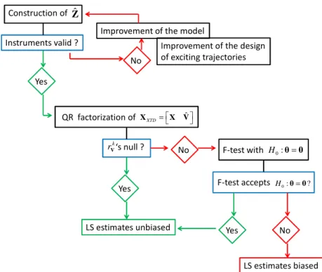
The Revised DWH-test is run as follows (see Fig. 1):
1. Construct the instrumental variable matrix Zˆ and validate/invalidate this construction with the
algorithm described in Section3.3.
2. If Zˆ is valid, calculate Vˆ =X−Zˆ .
3. Check with the QR decomposition of XXTD that θ has no influence on robot dynamics as explained
in Section3.2.
4. If the k
rV's are not null, assess the contribution of θ thanks to a F-test associated with H0:θ=0. If
the F-test accepts H0, then the LS estimates are considered as unbiased; otherwise, they are biased.
Fig. 1. Scheme of the Revised DWH-test suitable for robot identification
Compared with the classical regressed DWH-test, the Revised DWH-test can determine the origin of
Construction of Zˆ
Instruments valid ?
Yes
No
Improvement of the model
QR factorization of ˆ XTD= X X V ‘s null ? k rV Yes No LS estimates unbiased F-test with H0:θ=0 F-test accepts H0:θ=0? Yes No LS estimates biased Improvement of the design
the bias by evaluating the validity of the instruments, can detect a model misspecification and combines the QR factorization with a F-test. Those remarks make the proposed statistic relevant for mechatronic system identification.
4
Experimental Identification Results Obtained with the TX40
4.1
Model Reduction and Validation of the Statistical Hypotheses
Before presenting the experimental results obtained with the TX40 robot, the F-test used to eliminate the dynamic parameters having no effect on robot dynamics is first introduced. Then, the tests which validate/invalidate the statistical assumptions are presented.
4.1.1 F-test
Some dynamic parameters remain poorly identifiable because they are small. They can be cancelled to simplify the inverse and direct models. The most rigorous way consists in using the F-test
(Davidson and MacKinnon 1993) which is carried out with the weighted error ε=Ω−1/ 2ε. Because
( )
T 1/ 2( )
T 1/ 2 1/ 2 1/ 2r
E εε =Ω− E εε Ω− =Ω− ΩΩ− =I , it is assumed that ε∼Ν
(
0 I, r)
and the samples of ε areindependent. From b base parameters, bc parameters may define the set of essential parameters
that is enough to describe the robot dynamics. The F-test is performed as follows:
1. First, one runs the 2SLS method with the b base parameters and one computes ε ;
2. Second, one runs the 2SLS method with the bc essential parameters and one computes εc , the
error norm obtained with the reduced model; 3. Third, one calculates
(
)
(
)
(
)
2 2 2 ˆ c b bc F r b − − = − ε ε ε . (24) If Fˆ is less than (1 ) (,b bc) (,r b)F −α − − , the F-test accepts the model reduction; otherwise, it is rejected.
The F-test works if ε∼Ν
(
0 I, r)
holds and if the samples of ε are independent. These assumptionsmust be validated with the Kolmogorov-Smirnov test (KS-test) and the Durbin-Watson test (DW-test).
4.1.2 Kolmogorov-Smirnov test (KS-test)
The KS-test is a nonparametric test for equality of continuous one dimensional probability distribution that can be used to compare a sample with a reference probability distribution. The KS-test quantifies a distance between the empirical distribution function (EDF) of the sample and the cumulative distribution function (CDF) of the reference distribution. In our case, the null hypothesis is
(
)
0: , r
H ε∼Ν 0 I . The EDF of ε is compared with the CDF of the reference distribution via a KS-test
4.1.3 DW-test
Assuming ε∼Ν
(
0 I, r)
, the DW-statistic is given by( ) ( )
(
)
2( )
2(
)
1 2 1 1 2 1 r r i i dw ε i ε i ε i ρ = = =∑
− −∑
≈ − , (25)where ρ1 is the sample autocorrelation and ε
( )
i is the ith
sample of ε.
The value of dw lies between 0 and 4. dw=2 indicates no autocorrelation i.e. ρ1=0 and if the
DW-statistic is substantially less than 2, there is evidence of positive serial correlation. Small values of dw
indicate that successive error terms are close in value to one another (or positively correlated).
Similarly, if dw is greater than 2, successive error terms are much different in value from one another
(negatively correlated).
For robot identification, as a rough rule of thumb, if dw varies between 1.8 and 2.2, ε can be
considered as serially uncorrelated. Otherwise, a suspicion of a serial correlation is legitimate.
4.1.4 KS-test, Wald-test and F-test with MATLAB
In order to perform the KS-test, the kstest MATLAB function is used. The level of significance α is 5%.
It is recommended to calculate the p-value in order to make a good interpretation of the result. To perform the Wald-test, (23) is first calculated and the chi2cdf MATLAB function is used. For
instance, with (23), the following instruction is used
( )
2ˆ
1 2 ,
p= −chi cdf η b
δ where pis the p-value. It is
checked that p≥α to validate the set of instruments.
For the F-test, the fcdf MATALAB function is used. Fˆ given by (24) is first calculated and the
following instruction is used p= −1 fcdf F b bc r
(
ˆ, − , −b)
and if p≥α, the model reduction isvalidated.
4.2
Brief introduction of the TX40 Robot
The TX40 robot has a serial structure with six rotational joints and is characterized by a coupling
between the joints 5 and 6. This coupling adds two additional parameters: fvm6 the viscous friction
coefficient of motor 6 and fcm6 the dry friction coefficient of motor 6. The TX40 robot has 60 base
dynamic parameters. Its complete modelling is given in (Janot et al. 2014, a).
The robot is PD-controlled and τj is given by
(
)
(
)
j j j j j j j gτ kp qr qmes k qv mes τ = − − ɺ . (26) where j pk is the proportional gain in Nm/rad,
j
v
k is the derivative gain in Nm/(rad/s) ,
j
gτ is the drive gain and
j
mes
qɺ is the velocity calculated from the differentiation of
j
mes
The bandwidth of the first (resp. last) three position closed-loops is 10Hz (resp. 20 Hz). The results obtained with a PID controller sticking to those given in this paper, the use of a PD controller is enough and this is consistent with the results presented in (Gautier et al. 2013).
The reference trajectories
(
q q qr,ɺr,ɺɺr)
are designed so that qɺɺr are trapezoidal. Since(
)
(
ˆ , ,ˆ ˆ)
200cond X q q qɺ ɺɺ = ,
(
, ,)
r r r
q q qɺ ɺɺ excite well the base parameters (Gautier and Khalil 1992) and
(Pressé and Gautier 1993). To evaluate the three identification methods, data are stored with a
measurement frequency fm =5kHz.
To validate the estimates, cross-validations are performed. They are carried out with 3 fifth-order polynomials passing through points different from those defined to build the trajectories used to run the 3 identification methods. For cross-test validations, data are stored with a measurement
frequency cv 1
m
f = kHz and the relative errors are calculated with the LS or 2SLS estimates and with
these trajectories (see (Janot et al. 2014, a) for the details).
4.3
IDIM-LS method, 2SLS method and regressed DWH-test combined with
an appropriate bandpass filtering
The IDIM-LS method is carried out with a filtered position qˆ calculated with a 40 Hz fourth-order
Butterworth filter. For the three methods, the parallel decimation is carried out with a 10 Hz Tchebyshef filter.
Before calculating the LS and the 2SLS estimates, the construction of Zˆ is validated with the
procedure described in the subsection 3.3. The results are given in Table 1 where bj is the number of
identifiable parameters of a joint j. Because one has 2 2
( )
ˆ b
ηδ ≤χ with a p-value greater than 0.05, Zˆ
is valid and the 2SLS estimates are thus unbiased. For the columns associated with joint
accelerations, the ˆk
rV's are not null although very small (i.e. less than 1e-3) whereas for the columns
associated with joint positions and/or velocities only, the ˆ
k
rV's are null (smaller than 1e-20). A F-test
is therefore required to make a final decision.
TABLE 1:
RESULTS OF THE WALD-TEST (23) FOR EACH JOINT J
Joint j bj χ2
( )
bj max( )
ηˆδ2 p-value1 34 48.5 18.5 0.98 2 37 52.3 12.4 0.99 3 31 45.0 18.1 0.97 4 24 36.5 5.4 0.99 5 20 31.3 11.7 0.93 6 11 19.7 9.1 0.61
The first hypothesis ε∼Ν
(
0 I, r)
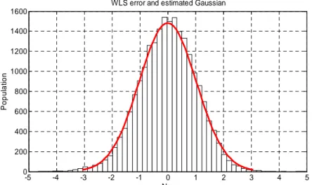
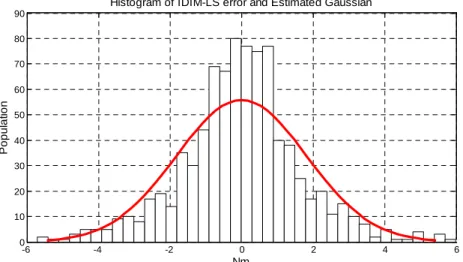
is validated with the KS-test with a level of significance α =0.05. Thedistribution of ε obtained with the IDIM-LS method and its estimated Gaussian are plotted in Fig. 3
(similar results are obtained with the two others methods). The KS-test accepts ε ∼Ν
(
0 I, r)
and thedistribution of ε matches a Gaussian distribution with the three methods. Furthermore, dw
calculated with (25) and given in Table 2 is close to 2.0 with the three methods. ε is thus serially
independent with ε∼Ν
(
0 I, r)
.The IDIM-LS and the 2SLS estimates are given in Table 2 as well the estimates ˆθ calculated with the
augmented DWH-test (NS stands for "Not Significant"). The F-test accepts to cancel the base
parameters such that %ˆˆ ( )
LSi σβ (resp. ( ) 2 ˆ ˆ % SLS i
σβ ) is greater than 30%. Actually, one obtains ε =48.5
with the whole model and εc =49with the reduced model. With b=60, bc =28 and r=2160, one
has Fˆ≈1.4 with a p-value greater than 0.05. From 60 base parameters, only 28 define a set of
essential dynamic parameters. Since the F-test accepts H0:θ=0, relation (15) holds, XXTD collapses
to X and
(
ˆ , ,ˆ ˆ)
(
, ,)
nf nf nf
≈
X q q qɺ ɺɺ X q qɺ qɺɺ . However, the 2SLS estimates are slightly less efficient than the
IDIM-LS estimates because one has
2 2
ˆ ˆ
ˆ ˆ
% %
SLS LS
σβ ≥ σβ for each estimate. This result is consistent with
the theory of Statistics (Wooldridge 2009).
Direct comparisons have been performed with the following relative errors: %relˆy = −y XβˆLS y for
the IDIM-LS method, %relˆy = −y Zβˆ2SLS y for revised DWH-test and for %relyˆ = −y XXTDβˆXTD y
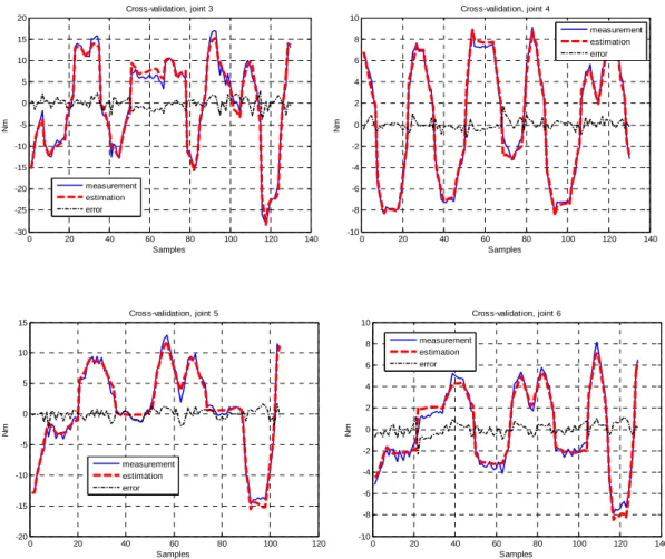
the regressed DWH-test. With relative errors close to 6% (see Table 2), the matching is therefore good. Cross-test validations have been performed. In Fig. 2, the torque reconstructed with the IDIM-LS estimates and with the second trajectory matches the measured one while the norm of the relative error calculated with each validation trajectory and with the IDIM-LS and the 2SLS estimates given in Table 3 stick to those calculated with the direct comparisons. The estimates can be considered as unbiased.
TABLE 2:
IDIM-LS AND 2SLS ESTIMATES,REGRESSED DWH-TEST ESTIMATES –APPROPRIATE DATA FILTERING
(
ˆ)
ˆ %ˆ LS LS σβ β(
)
2 ˆ 2 ˆ %ˆ SLS SLS σβ β ˆθ ZZ1R 1.26 (1.2%) 1.25 (1.3%) NS Fv1 8.1 (0.7%) 8.20 (0.7%) NI Fc1 6.60 (2.3%) 6.54 (2.6%) NI XX2R -0.48 (2.5%) -0.48 (2.9%) NS XZ2R -0.16 (4.4%) -0.16 (4.8%) NS ZZ2R 1.09 (1.1%) 1.09 (1.2%) NS MX2R 2.20 (2.5%) 2.21 (2.9%) NI Fv2 5.68 (1.1%) 5.68 (1.2%) NI Fc2 7.76 (1.8%) 7.77 (2.1%) NI XX3R 0.13 (9.5%) 0.13 (10.2%) NS ZZ3R 0.12 (7.6%) 0.12 (8.8%) NS MY3R -0.59 (2.2%) -0.59 (2.3%) NIIa3 0.084 (8.8%) 0.088 (9.2%) NS Fv3 2.02 (1.7%) 2.03 (1.8%) NI Fc3 6.10 (1.8%) 6.05 (1.9%) NI MX4 -0.02 (26.7%) -0.02 (30.0%) NI Ia4 0.029 (8.8%) 0.029 (9.4%) NS Fv4 1.14 (1.5%) 1.15 (1.5%) NI Fc4 2.34 (2.6%) 2.27 (2.6%) NI MY5R -0.03 (13.7%) -0.03 (14.1%) NI Ia5 0.044 (8.9%) 0.041 (11.2%) NS Fv5 1.87 (1.8%) 1.92 (2.0%) NI Fc5 2.93 (3.0%) 2.79 (3.5%) NI Ia6 0.01 (9.4%) 0.01 (10.9%) NS Fv6 0.67 (1.5%) 0.69 (1.6%) NI Fc6 2.08 (2.5%) 2.00 (2.8%) NI fvm6 0.63 (1.6%) 0.63 (1.8%) NI fcm6 1.80 (3.7%) 1.81 (4.2%) NI ˆ %rely 6.0% 6.0% 6.0% dw 1.8 1.9 1.9 TABLE 3:
RELATIVE ERRORS OBTAINED WITH CROSS-VALIDATION, THE IDIM–LS AND THE 2SLS ESTIMATES
cv m f %relyˆ (LS) %relyˆ (2SLS) Trajectory 1 1 kHz 6.5% 6.5% Trajectory 2 1 kHz 6.5% 6.5% Trajectory 3 1 kHz 7.0% 7.0% 0 20 40 60 80 100 120 140 -80 -60 -40 -20 0 20 40 60 80 Cross-validation, joint 1 N m Samples measurement estimation error 0 20 40 60 80 100 120 140 -80 -60 -40 -20 0 20 40 60 Cross-validation, joint 2 N m Samples measurement estimation error
Fig. 2. Cross-validations, joints 1, 2, 3, 4, 5 and 6 with 2SLS estimates and with the first trajectory. Blue: measurement; red: estimation; black: error. Appropriate data filtering. The constructed torques stick to the measured ones. Similar results are obtained with the IDIM-LS method.
Fig. 3. Histogram of IDIM-LS error and its estimated Gaussian – Appropriate data filtering. The distribution matches a Gaussian distribution. A similar result is obtained with the 2SLS method.
0 20 40 60 80 100 120 140 -30 -25 -20 -15 -10 -5 0 5 10 15 20 Cross-validation, joint 3 N m Samples measurement estimation error 0 20 40 60 80 100 120 140 -10 -8 -6 -4 -2 0 2 4 6 8 10 Cross-validation, joint 4 N m Samples measurement estimation error 0 20 40 60 80 100 120 -20 -15 -10 -5 0 5 10 15 Cross-validation, joint 5 N m Samples measurement estimation error 0 20 40 60 80 100 120 140 -10 -8 -6 -4 -2 0 2 4 6 8 10 Cross-validation, joint 6 N m Samples measurement estimation error -5 -4 -3 -2 -1 0 1 2 3 4 5 0 10 20 30 40 50 60 70 80 90 100
WLS error and estimated Gaussian
Nm P o p u la ti o n
4.4
IDIM-LS method, 2SLS method and the regressed DWH-test combined
with an inappropriate data filtering
In this section, the robustness of the methods against an inappropriate data filtering is studied. The
IDIM-LS and 2SLS methods are carried out with the position qˆ filtered with a 200 Hz fourth-order
Butterworth filter and with velocities qɺˆ and accelerations qɺɺˆ, calculated with a central difference
algorithm of qˆ. The parallel decimation is carried out with a lowpass Tchebyshef filter with a cutoff
frequency of 100 Hz.
Because one has 2 2
( )
ˆ b
ηδ ≤χ with a p-value greater than 0.05, Zˆ is valid and the 2SLS estimates are
thus unbiased. In that case, the ˆ
k
rV's associated with joint accelerations are of the same magnitude
as those of the k
rX's. With the IDIM-LS method, the 2SLS method and the regressed DWH-test, the
KS-test accepts the hypothesis ε∼Ν
(
0 I, r)
with a level of significance α =0.05 while dw is close to2.0 (see Table 4). Finally, it comes out that ε is serially independent with ε∼Ν
(
0 I, r)
.The estimates of the IDIM-LS, the 2SLS methods and the regressed DWH-test are given in Table 4 (only the significant parameters are given). At first glance, the IDIM-LS estimates seem acceptable
because they are not aberrant, the relative error %relyˆ is not critical and the histogram of IDIM-LS
error plotted in Fig. 4 matches a Gaussian distribution. Unfortunately, they are biased since they do not stick to the 2SLS estimates while the observed differences are not spanned by the LS variances
and θ contributes to the dynamics, the F-test rejecting H0:θ=0. The 2SLS estimates obtained with
an inappropriate data filtering are less efficient than those obtained with an appropriate data filtering, their relative deviations being four/five times greater. This result highlights the behaviour of IV estimators: they are able to provide unbiased estimates with very large deviations. This result is consistent with the theory of Statistics (Wooldridge 2009).
All the components of θˆ corresponding to inertia parameters (ZZ1R, XX2R, XZ2R, ZZ2R, XX3R, ZZ3R, Ia3, Ia4,
Ia5, Ia6) and to some gravity parameters (MY3R, MX4, MY5R) are identifiable and have a significant
contribution because the F-test rejects H0:θ=0. This is due to the fact that their associated
columns contain noisy joint accelerations. The augmented DWH-test supports the results of the
Revised DWH-test (the estimates of the regressed DWH-test are not given because they stick to βˆ2SLS
).
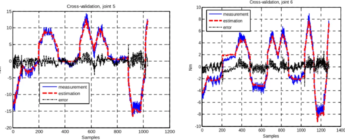
Cross-test validations have been performed and the results obtained with the second trajectory and the IDIM-LS estimates are plotted in Fig. 5. Despite the fact that the errors are not negligible, the reconstruction of torques is quite acceptable and the IDIM-LS estimates are acceptable for a non-expert in system identification. This result shows that the cross-validations may be not enough to make a final decision. In Table 5, the norms of relative errors calculated with the set of trajectories and with the IDIM-LS (resp. the 2SLS) estimates are given. With the 2SLS estimates, these relative errors match those calculated with the direct comparisons whereas there are some differences with the IDIM-LS estimates although these differences are not as critical as expected. Without running the Revised DWH-test, there are no undisputable evidences to conclude that the IDIM-LS estimates are biased.
Fig. 4. Histogram of IDIM-LS error with its estimated Gaussian – Inappropriate data filtering. The error distribution matches a Gaussian distribution.
TABLE 4:
IDIM-LS AND 2SLS ESTIMATES,REGRESSED DWH-TEST RESULTS –INAPPROPRIATE DATA FILTERING
(
ˆ)
ˆ %ˆ LS LS σβ β(
)
2 ˆ 2 ˆ %ˆ SLS SLS σβ β θˆ( )
%σˆθˆ ZZ1R 1.11 (0.8%) 1.24 (4.1%) -1.22 (3%) Fv1 8.23 (0.5%) 8.25 (2.4%) NS Fc1 6.42 (1.7%) 6.38 (9.1%) NS XX2R -0.38 (1.9%) -0.48 (10.6%) 0.46 (9%) XZ2R -0.16 (3.0%) -0.16 (15.9%) 0.14 (16%) ZZ2R 0.88 (0.8%) 1.08 (3.8%) -1.0 (3%) MX2R 2.42 (1.7%) 2.22 (9.9%) NS Fv2 5.63 (0.8%) 5.75 (4.4%) NS Fc2 7.88 (1.3%) 7.55 (6.4%) NS XX3R 0.19 (5.7%) 0.13 (29.3%) -0.11 (20%) ZZ3R 0.07 (6.2%) 0.11 (28.8%) -0.12 (10%) MY3R -0.71 (1.0%) -0.60 (6.6%) 0.5 (6%) Ia3 0.15 (2.6%) 0.09 (24.5%) -0.07 (20%) Fv3 2.03 (1.0%) 2.01 (4.5%) NS Fc3 5.96 (1.1%) 5.83 (5.1%) NS MX4 -0.01 (20.1%) -0.02 (27.5%) 0.01 (50%) Ia4 0.022 (3.9%) 0.028 (25.5%) NS Fv4 1.14 (0.6%) 1.17 (3.2%) NS Fc4 2.35 (1.0%) 2.23 (6.3%) NS MY5R -0.02 (5.7%) -0.03 (28.3%) 0.03 (9%) Ia5 0.02 (3.2%) 0.04 (25.2%) -0.03 (12%) Fv5 1.84 (0.7%) 1.94 (4.0%) NS Fc5 3.01 (1.1%) 2.72 (7.3%) NS Ia6 0.007 (3.3%) 0.01 (24.5%) -0.008 (10%) Fv6 0.67 (0.6%) 0.69 (3.8%) NS Fc6 2.11 (1.0%) 1.97 (6.2%) NS fvm6 0.63 (0.6%) 0.64 (3.8%) NS fcm6 1.80 (1.4%) 1.74 (8.1%) NS -5 -4 -3 -2 -1 0 1 2 3 4 5 0 200 400 600 800 1000 1200 1400 1600WLS error and estimated Gaussian
Nm P o p u la ti o n
ˆ
%rely 17.0% 12.5% 11.0%
dw 1.7 1.8 1.8
TABLE 5:
RELATIVE ERRORS OBTAINED WITH CROSSCHECKING,IDIM–LS AND 2SLS ESTIMATES
cv m f %relyˆ (LS) %relyˆ (2SLS) Trajectory 1 1 kHz 20.0% 14.0% Trajectory 2 1 kHz 22.0% 14.0% Trajectory 3 1 kHz 21.0% 14.5% 0 200 400 600 800 1000 1200 1400 -80 -60 -40 -20 0 20 40 60 80 Cross-validation, joint 1 N m Samples measurement estimation error 0 200 400 600 800 1000 1200 1400 -100 -80 -60 -40 -20 0 20 40 60 80 Cross-validation, joint 2 N m Samples measurement estimation error 0 200 400 600 800 1000 1200 1400 -50 -40 -30 -20 -10 0 10 20 30 Cross-validation, joint 3 N m Samples measurement estimation error 0 200 400 600 800 1000 1200 1400 -15 -10 -5 0 5 10 15 Cross-validation, joint 4 N m Samples measurement estimation error
Fig. 5. Cross-validations, joints 1, 2, 3, 4, 5 and 6 with IDIM-LS estimates and with the second trajectory. Blue: measurement; red: estimation; black: error. Inappropriate data filtering. The matching is quite good despite the fact that the IDIM-LS estimates are biased.
4.5
Robustness against a misspecified model
The robustness of the Revised DWH-test against a misspecified model is now studied. Because the gear ratios are greater than 25, it is legitimate to assume that the parameters of gravity and the off-diagonal elements of inertia matrices do not contribute significantly to the dynamics. These parameters and their associated columns are removed from the IDM. The data are filtered as explained in Section 4.3.
For the inertia parameters of joints 1, 2, 3 and 4, the Wald-test rejects the hypothesis that Zˆ is valid
because the minimum of 2
ˆ
ηδ given in Table 6 is greater than 2
( )
j
b
χ while the p-value is almost null.
Interestingly, the set of instruments of joint 5 and 6 is valid. This is mainly due to the fact that the
gravity parameters and the off-diagonal elements of inertia matrices are practically null. Because Zˆ
is not valid, the 2SLS estimates are biased.
The IDIM-LS and 2SLS estimates given in Table 7 differ from those given in Table 2. They are
therefore biased. The KS-test rejects the hypothesis ε∼Ν
(
0 I, r)
for both methods. The IDIM-LS errorand its estimated Gaussian are plotted in Fig. 6 and the distribution does not match a Gaussian distribution (a similar result is obtained with the 2SLS method). This experiment shows that the Revised DWH-test is able to detect a model misspecification.
TABLE 6:
RESULTS OF THE WALD-TEST (23) FOR THE JOINTS 1,2,3 AND 4–MISSPECIFIED MODEL –APPROPRIATE DATA FILTERING
Joint j bj χ2
( )
bj min( )
ηδˆ2 p-value0 200 400 600 800 1000 1200 -20 -15 -10 -5 0 5 10 15 Cross-validation, joint 5 N m Samples measurement estimation error 0 200 400 600 800 1000 1200 1400 -10 -8 -6 -4 -2 0 2 4 6 8 10 Cross-validation, joint 6 N m Samples measurement estimation error
1 3 7.81 16.3 ~0 2 3 7.81 19.1 ~0 3 4 9.5 25.7 ~0 4 4 9.5 19.6 ~0 5 4 9.5 5.1 0.28 6 6 12.59 4.9 0.56 TABLE 7:
IDIM-LS ESTIMATES AND 2SLS ESTIMATES –MISSPECIFIED MODEL AND APPROPRIATE DATA FILTERING
(
ˆ)
ˆ %ˆ LS LS σβ β(
)
2 ˆ 2 ˆ %ˆ SLS SLS σβ β ZZ1R 1.10 (3.0%) 1.08 (3.5%) Fv1 8.16 (3.0%) 8.17 (3.6%) Fc1 6.50 (10.6%) 6.48 (11.0%) ZZ2R 1.37 (2.3%) 1.20 (2.0%) Fv2 5.80 (5.2%) 5.83 (5.8%) Fc2 6.80 (10.3%) 6.80 (11.0%) ZZ3R 0.31 (7.8%) 0.27 (6.7%) Ia3 0.05 (36.0%) 0.07 (40.0%) Fv3 2.21 (7.2%) 2.22 (7.6%) Fc3 5.55 (9.3%) 5.53 (9.5%) Ia4 0.04 (26.2%) 0.05 (31.1%) Fv4 1.18 (5.0%) 1.20 (5.8%) Fc4 2.20 (9.6%) 2.17 (10.0%) Ia5 0.06 (28.2%) 0.05 (29.3%) Fv5 1.90 (7.1%) 1.89 (7.3%) Fc5 2.75 (12.5%) 2.75 (12.6%) Ia6 0.01 (31.0%) 0.01 (33.0%) Fv6 0.69 (5.1%) 0.69 (5.4%) Fc6 2.0 (8.9%) 2.0 (9.3%) fvm6 0.64 (5.6%) 0.64 (5.9%) fcm6 1.70 (15.2%) 1.70 (16.0%) ˆ %rely 17.0% 21.0% dw 1.8 1.8Fig. 6. Histogram of IDIM-LS error and its estimated Gaussian – Appropriate data filtering – Misspecified dynamic model
5
Conclusion
In this paper, a Revised DWH-test suitable for identification of robots was introduced and experimentally validated on a 6 degrees-of-freedom industrial robot. The main contributions of the work presented in this paper are the following:
• The Revised DWH-test can validate/invalidate the instruments chosen by the user and is
based on general statistical assumptions,
• The Revised is able to detect model misspecifications,
• The algorithm makes use of the QR factorization of an augmented matrix and is combined
with a F-test if required,
• The Revised DWH-test is able to validate/invalidate IDIM-LS estimates.
The results provided by the revised statistic were cross-validated and compared with those provided by the augmented DWH-test widely used in Econometrics. Since all the results are close to each others, this shows that the results provided by the Revised DWH-test are reliable.
Future works will address the application of the Revised DWH-test on flexible robots and electrical motors. The calculation of the optimal prefilters for robot identification and the application of the experiment design are worth of investigation and will be addressed.
6
References
Aguero and Goodwin (2006), "On the Optimality of Open and Closed Loop Experiments in System Identification," In: Proceedings of the 45th IEEE Conference on Decision and Control Conference, 2006, Page(s): 163 – 168
Aguero and Goodwin (2007), "Choosing between open- and closed-loop experiments in linear system identification," IEEE Transactions on Automatic Control, Vol. 52(8), August 2007, pp. 1475-14780
-6 -4 -2 0 2 4 6 0 10 20 30 40 50 60 70 80 90 Nm P o p u la ti o n
Calanca A., Capisani L. M., Ferrara A., and Magnani L. (2011), “MIMO Closed Loop Identification of an Industrial Robot,” IEEE Transactions on Control System Technology, Vol. 19(5), September 2011, pp. 1214-1224.
Chen F., Garnier, H. and Gilson, M., Robust identification of continuous-time models with arbitrary time-delay from irregularly sampled data (2015), Journal of Process Control, vol. 25, pp. 19-27, January 2015.
Davidson R. and MacKinnon J.G. (1993), “Estimation and Inference in Econometrics,” Oxford University Press, New York, 1993.
Dellon B. and Matsuoka Y. (2009), “Modeling and System Identification of a Life-Size Brake-Actuated Manipulator,” IEEE Transactions on Robotics, vol. 25(3), June 2009, pp. 481 – 491.
Garnier H. and Wang L. (2008), “Identification of Continuous-time Models from Sampled Data,” Springer, 2008.
Gautier M. (1991), “Numerical calculation of the base inertial parameters,” Journal of Robotics Systems, vol. 8, no. 4, pp. 485-506, 1991.
Gautier M. and Khalil W. (1992), “Exciting trajectories for the identification of the inertial parameters of robots,” International Journal of Robotics Research, vol. 11, Aug. 1992, pp. 362-375.
Gautier M. and Poignet P. (2001), “Extended Kalman Filtering and Weighted Least-squares Dynamic Identification of Robot,” Control Engineering Practice, vol. 9, 2001, pp. 1361-1372.
Gautier M., Janot A., and Vandanjon P.O., (2013), “A New Closed-Loop Output Error Method for Parameter Identification of Robot Dynamics,” IEEE Transactions on Control System Technology, vol. 21(2), March 2013, pp. 428-444.
Gilson M., Garnier H., Young P.C. and Van den Hof P. (2011), “Optimal instrumental variable method for closed-loop identification”, Control Theory & Applications, IET, vol. 5(10), pp. 1147 – 1154.
Hausman J.A. (1978), “Specification Tests in Econometrics,” Econometrica, vol. 46(6), 1978, pp. 1251 – 1271.
Hollerbach J., Khalil W., and Gautier M. (2008), “Model Identification,” Springer Handbook of Robotics, Springer, 2008.
Indri M., Calafiore G., Legnani G., Jatta F. and Visioli A. (2002), “Optimized Dynamic Calibration of a SCARA Robot,” In: Proceedings of the 15th IFAC World Congress, July 2002, Barcelona, Spain.
Janot A., Vandanjon P.O. and Gautier M. (2013), “A Durbin-Wu-Hausman Test for Industrial Robots Identification,” In: Proc. of IEEE International Conference on Robotics and Automation, Karlsruhe, Germany, May 2013, pp. 2956-2961.
Janot A., Vandanjon P.O. and Gautier M. (2014, a), “A Generic Instrumental Variable Approach for Industrial Robots Identification,” IEEE Transactions on Control Systems Technology, Vol. 22(1), pp.132-145, January 2014.