HAL Id: hal-01714856
https://hal.archives-ouvertes.fr/hal-01714856
Submitted on 23 Feb 2018
HAL is a multi-disciplinary open access
archive for the deposit and dissemination of
sci-entific research documents, whether they are
pub-lished or not. The documents may come from
teaching and research institutions in France or
abroad, or from public or private research centers.
L’archive ouverte pluridisciplinaire HAL, est
destinée au dépôt et à la diffusion de documents
scientifiques de niveau recherche, publiés ou non,
émanant des établissements d’enseignement et de
recherche français ou étrangers, des laboratoires
publics ou privés.
Dynamic Obstacle Avoidance Strategies using Limit
Cycle for the Navigation of Multi-Robot System
Ahmed Benzerrouk, Lounis Adouane, Philippe Martinet
To cite this version:
Ahmed Benzerrouk, Lounis Adouane, Philippe Martinet. Dynamic Obstacle Avoidance Strategies
using Limit Cycle for the Navigation of Multi-Robot System. 2012 IEEE/RSJ IROS’12, 4th
Work-shop on Planning, Perception and Navigation for Intelligent Vehicles, Oct 2012, Vilamoura, Algarve,
Portugal. �hal-01714856�
Dynamic Obstacle Avoidance Strategies using Limit Cycle for the
Navigation of Multi-Robot System
A. Benzerrouk
1, L. Adouane
2and P. Martinet
3 1Institut Français de Mécanique Avancée, 63177 Aubière, France
2 Clermont Université, Université Blaise Pascal, BP 10448, 63000 Clermont-Ferrand, France 3
IRCCYN, Ecole Centrale de Nantes, 1 rue de la Noé, BP 92101, 44321 Nantes Cedex 03, France
Abstract— This paper deals with the navigation of a multi-robot system (MRS). The latter must reach and maintain a specific formation in dynamic environment. In such areas, the collision avoidance between the robots themselves and with other obstacles (static and dynamic) is a challenging issue. To deal with it, a reactive and a distributed control architecture is proposed. The navigation in formation of the MRS is insured while tracking a global virtual structure. In addition, according to the robots’ perception context (e.g., static or dynamic obstacle), the most suitable obstacle avoidance strategy is activated. These approaches use mainly the limit-cycle principle and a penalty function to obtain linear and angular robots’ velocities. The proposed control law guarantees the stability (using Lyapunov function) and the safety of the MRS. The robustness and the efficiency of the proposed control architecture is demonstrated through a multitude of experiments which shows the MRS in different configuration of avoidance.
I. INTRODUCTION
Navigation of multiple mobile robots is a recurrent re-search subject due to a large amount of the met issues. Obstacle avoidance is among the most important ones. In fact, it is a basic action that each mobile robot has to accomplish in its environment in order to prevent collision (with walls, trees, walkers, other robots, etc.), and to insure a safe navigation.
Collision avoidance is then widely investigated in the literature for multi-robot systems. It is tackled through two main approaches. The first one considers the robots control, entirely based on path planning methods which involve the prior knowledge of the robots environment. The objective is to find the best path to all the robots in order to avoid each other while minimizing a cost function [1], [2], [3]. This method requires a significant computational complexity, especially when the environment is highly dynamic. In fact, the robot has to frequently replan its path to take environment changes into account.
Rather than a prior knowledge of the environment, reactive methods are based on local robots sensors information. At each sample time, robot’s control is computed according to its perceived environment. Potential field methods [4] are the most common ones: each robot is subject to a sum of an attractive virtual force generated by the goal to reach and repulsive forces generated by the other robots
and obstacles [5], [6], [7]. An other reactive method is the Deformable Virtual Zone (DVZ) [8]: every robot is surrounded by a virtual risk area. If an obstacle enters inside this DVZ, it deforms it. The aim of the generated control is then to minimize this deformation leading to avoid collision among robots [9]. The reactive methods given above suffer from local minima problems when for instance, the sum of potential forces is null, or when the deformation of the DVZ is symmetric (as the U shape obstacle). In [10], authors propose the Distributed Reactive Collision Avoidance algorithm (DRCA). This method is based on an equilibrium point which continuously pushes the robots away from each other by increasing their relative velocities. Hence, this algorithm is not suitable for the navigation in formation where robots regularly have to move with the same velocity. Generally, reactive methods do not require high computational complexities, since robots actions must be given in real-time according to the perception.
This paper deals with this last kind of methods. The studied task is the navigation in formation. It is accomplished through a distributed control architecture. This architecture was developed in [11] and permits for a group of mobiles robots to reach and maintain a specific formation. In this last work, obstacle avoidance was not addressed neither for dynamical obstacles nor to avoid other robots participating in the formation. In [11] the used strategy deals with the virtual structure. The formation is considered as a virtual rigid body and the control law for each robot is derived by defining the dynamics of this body [6], [12], [13]. Virtual structure is often associated to potential field applications since they are simple and allow collision avoidance. However, potential forces are limited, especially when the formation shape needs to be frequently reconfigured. In fact, it means that the robot is submitted to a frequently-changing number/amplitude of forces leading to more local minima, oscillations, etc. Hence, it was proposed that the robots track a virtual body without using potential forces. Since collision avoidance must stay possible despite the absence of potential fields, behavior-based concept [14], [15] was introduced. This allows to divide the task into two different behaviors (controllers):
attraction to a dynamic target, and obstacle avoidance. The
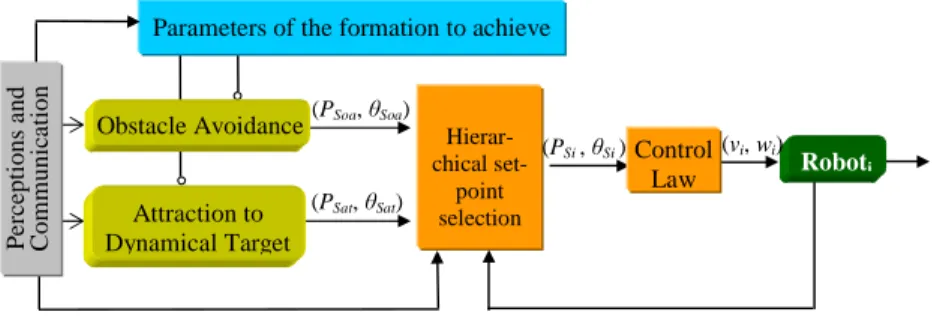
Hierar- chical set-point selection Attraction to Dynamical Target Roboti (PSoa, θSoa) (PSi , θSi ) Control Law (vi, wi) P e rc ept ions a nd C om m uni ca ti on inf or m at
ion Obstacle Avoidance
Parameters of the formation to achieve
(PSat, θSat)
Fig. 1. The proposed architecture of control embedded in each robot.
Limit-cycle navigation was already used for obstacle avoid-ance [17], [18]. Limit-cycle approach allows to choose the obstacle avoidance direction (clockwise or counterclockwise) in order to rapidly join the assigned target. Here, it is proposed to extend this method to dynamic obstacles and to robots of the same system without loosing the control reactivity. Unlike most of algorithms addressing dynamic obstacles, no communication is required among the robots to accomplish the task. Avoidance is based only on the local perception of each robot. As in [19], [18] or [20] the idea is to find the best direction of avoidance. It will be seen that the velocity vector of the obstacle is sufficient to deduce this direction.
The remainder of the paper is organized as follows. Sec-tion II gives the principle of the navigaSec-tion in formaSec-tion and the general control architecture. Basic controllers and the the control law are given in this section. We mainly focus on the obstacle avoidance controller applied to dynamic obstacles. In section III, a penalty function is introduced in the linear velocity of each robot to permits to take into account the multi-robot interactions. Section IV validates the proposed algorithm with experimental results. Finally, we conclude and give some perspectives in section V.
II. CONTROLARCHITECTURE
The used control architecture includes two controllers: Attraction to a Dynamic Target and Obstacle Avoidance. The virtual structure is built through the Parameters of the
Formation to Achieve block (cf. Figure 1).
According to environment information collected by the
Perceptions and Communication block (sensors) and the
robot’s current state, one controller is chosen thanks to the
Hierarchical Set-Point Selection block.
The corresponding set-points(PSi, θSi) (position and
ori-entation) are then sent to the Control Law block which
calculates the linear and angular velocities noted vi and wi
respectively (cf. Figure 1).
A. Parameters of the Formation to Achieve block
This subsection briefly describes the adopted virtual
struc-ture principle. Consider N robots with the objective of
reaching and maintaining them in a given formation. The proposed virtual structure that must be followed by the group of robots is defined as follow:
• Define one point which is called the main dynamic
target (cf. Figure 2),
• Define the virtual structure to follow by defining NT
nodes (virtual targets) to obtain the desired geometry.
Each nodei is called a secondary target and is defined
according to a specific distanceDi and angle Φi with
respect to the main target. Secondary targets defined by
this way have then the same orientationθT. However,
each target i will have its linear velocity vTi. The
number of these targetsNT must beNT ≥ N .
A cooperative strategy between the robots allows to each one to choose the closest target by negotiating it with the others thanks to Relative Cost Coefficients. To focus mainly on obstacle avoidance, this strategy is deactivated. Each robot
i has then to track a predefined target i. An exemple to get
a triangular formation is given in figure 2.
Di Dj j T Ow Xw Yw Main dynamical target Secondary target vT Dk k i Robotq Robotp Robotr
Fig. 2. Keeping a triangular formation by defining a virtual geometrical structure.
B. Attraction to a Dynamic Target controller
To remind the attraction to a Dynamic Target Controller
which allows to keep the formation, consider a robot i
with(xi, yi, θi) pose. This robot has to track its secondary dynamic target. To simplify notations in the following, the same subscript of the robot is given to its target. The latter
is then notedTi(xTi, yTi, θT) (cf. Figure 3) and the variation
of its position can be described by
(
˙xTi = vTi.cos(θT)
˙yTi = vTi.sin(θT)
(1) Let’s also introduce the used robot model (cf. Figure 3). Experimental results are made on Khepera robots, which are unicycle mobile robots. Their kinematic model can be described by the well-known equations (cf. Equation 2).
i Ym Xm Om(xi , yi) dSi Ow Xw Yw i T vTi Ti (xTi , yTi ) Secondary Virtual Target
Fig. 3. Attraction to a dynamic target.
˙xi= vi.cos(θi) ˙yi= vi.sin(θi) ˙ θi= ωi (2)
whereθi, vi andωi are respectively the robot orientation,
the linear and angular velocities.
The set-point angle that the robot must follow, to reach its dynamic target, is given by
θSati = arcsin(b sin(θT − γi)) + γi (3)
Whereb= vTi
vi .γi is the angle that the robot would have
if it was directed to its target (cf. Figure 3). This set-point
has been obtained by keepingγi constant. More details and
proofs are available in [11].
The corresponding set-points (PSi, θSi) (cf. Figure 1)
given by the Attraction to Dynamic Target controller are composed by:
• (PSi= (xTi, yTi)): the current position of the dynamic
target (cf. Figure 3),
• (θSi = θSati) given by equation (3).
C. Obstacle Avoidance controller
A particular attention is given to this task since the objective of the paper is to extend the already proposed orbital obstacle avoidance strategy [18], so that it becomes more appropriate to deal with dynamic obstacles. As cited in section I, common potential field approaches for obstacle avoidance are not used because of their drawbacks in robots formation. The task is then performed through the limit cycle methods. The robot follows the limit cycle vector fields described by the following differential equations:
˙xs = (sign)ys+ xs(R2I− x2s− y2s)
˙ys = −(sign)xs+ ys(R2I− x2s− ys2)
(4)
where (xs, ys) corresponds to the relative position of
the robot according to the center of the convergence circle
(characterized by anRI radius).
The function sign allows to define the direction of the
trajectories described by these equations. Hence, two cases are possible
• sign= 1, the motion is clockwise.
• sign= −1, the motion is counterclockwise.
Figure 4 shows the limit cycles with a radius RI = 1.
Obstacles are then modeled as circles ofRI radius. The latter
is chosen as the sum of the obstacle radius, the robot radius and a safety margin.
The set-point angleθSoa of the Obstacle Avoidance
con-troller is given by the the following relation
θSoa= arctan(
˙ys
˙xs
) (5)
The corresponding set-points(PSi, θSi), when the
Obsta-cle Avoidance controller is chosen by Hierarchical Set-Point Selection block (cf. Figure 1), are defined such that PSoa
corresponds to the center position of the obstacle (xo, yo)
whereasθSi = θSoa.
It is noticed that previous works on limit-cycle methods applied to obstacle avoidance [17], [18] do not consider dynamic obstacles. Here, it is proposed to extend this reactive method to deal with them.
According to the nature of the obstacle, three cases are considered:
1) static obstacles, 2) dynamic obstacles, 3) robots of the same system.
These strategies are explained in the next paragraphs.
1) Static obstacles: The same strategy proposed in [18]
is maintained. Summarily, the value ofsign is specified by
the ordinate of the robotys in the relative obstacle’s frame
(OoXoYo) (cf. Figure 5). The Xo axis of this orthonormal frame is defined thanks to two points: the center of the obstacle (which makes the origin of the frame) and the target to reach. sign = ( 1 ifys≥ 0 (clockwise avoidance) −1 ifys<0 (counterclockwise avoidance) (6) Figure 5 shows an example of a robot choosing its avoidance direction (clockwise) thanks to its relative ordinate
ys > 0. The chosen direction by this strategy allows then to join the target by the side offering the smallest covered distance.
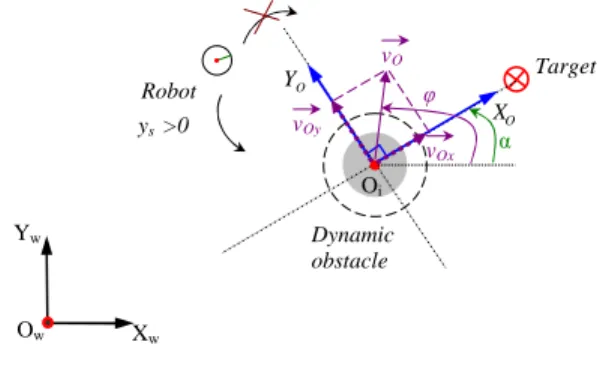
2) Dynamic obstacles: When a movement of the obstacle
position is detected, it is considered as a dynamic obstacle by the robot. The objective for the robot is always to choose the most suitable side of avoidance (clockwise or counterclockwise) which allows to succeed this mission. The
proposed solution is always to act on the function sign
(cf. Equation 4). Nevertheless, for dynamic obstacles, the
ordinate ys cannot be used as the adequate information to
-3 -2 -1 0 1 2 3 -3 -2 -1 0 1 2 3 x s ys (a) Clockwise (sign = 1) -3 -2 -1 0 1 2 3 -3 -2 -1 0 1 2 3 x s ys (b) Counter-Clockwise (sign = −1)
ys >0 Static obstacle Target Robot YO O X Ow Xw Yw Oi α Circle of influence with RI radius
Fig. 5. Avoiding a static obstacle.
decide on the avoidance direction. In figure 6, it can be noticed that if the robot decides a clockwise motion (based
on its relative positive ordinateys>0), it fails to avoid this
obstacle. In fact, the robot will go in the same direction as
the obstacle (vector~vO on the figure). It may then uselessly
diverge from its target by persisting in this direction.
ys >0 φ vOx Dynamic obstacle Target Robot YO O X Ow Xw Yw Oi α vO vOy
Fig. 6. Avoiding a dynamic obstacle.
Rather than analyzingys, it is then proposed that the robot
uses the obstacle’s vector velocity~vO. The idea is to project
this vector on the Yo axis of the relative frame (OoXoYo)
defined in paragraph II-C.1. Noted vOy, this projection is
expressed as v
Oy = vOsin(ϕ − α) (7)
whereα and ϕ define the direction of the Xoaxis and~vO
in the absolute frame respectively. The function sign (cf.
Equation 4) is then defined according tovOy as follows:
sign = (
1 ifvOy ≤ 0 (clockwise avoidance)
−1 ifvOy >0 (counterclockwise avoidance)
(8)
By using the projection vOy of the obstacle velocity, the
obstacle is always avoided round the back such that the robot does not cut off the obstacle’s trajectory.
3) Robots of the same system: One can consider that
every robot of the MRS is treated as a dynamic obstacle and projects its velocity vector to deduce the side of avoidance (cf. Equation 8). However, a conflict problem could appear when, for instance, two robots have to avoid each other. Once each robot projects the velocity vector of the other one, they have opposite directions of motion. They can endlessly hinder each other which leads to divergence from their
targets. This problem is illustrated by a simulation example in figure 7. 2 4 6 8 10 12 14 15 16 17 18 19 20 21 22 23 24 25
Robot trajectory in the [O, X, Y] reference
X [m] Y [ m ] Target robot1 Target robot2 Target robot1 Robot2 Robot1
Fig. 7. Divergence of the robots from their targets due to two different directions of avoidance.
To deal with this kind of conflicts, and assuming that each robot is able to identify those of the same system, it is proposed to impose one reference direction for all the system. Hence, when one robot detects a disturbing robot of the same group, it avoids it counterclockwise.
D. The control law block
This block allows for the robot i to converge to its
set-point given by the Hierarchical set-set-point selection block(cf. Figure 1). It is expressed as vi = vmax− (vmax− vT)e−(d 2 Si/σ2) (9a) ωi= ωSi+ k1θ˜i (9b) where
• vmax is the maximum linear speed of the robot,
• σ, k1 are positive constants,
• vi andωi are linear and angular velocities of the robot.
wSi = ˙θSi.
˜
θi = θSi− θi (10)
where θSi is the set-point angle according to the active
controller and was already computed (cf. Equation (3), (5)). By derivating
˙˜θi= wSi− ωi (11)
Consider the well known Lyapunov function V=12θ˜i
2
(12)
The angular control law is asymptotically stable if ˙V <0.
˙
V = k1θ˜i˙˜θi
By replacing equation (11) in the control law (9b), we get
˙˜θi= −k1θ˜i
and ˙V becomes V˙ = −k1θ˜2
i <0
for every ˜θi6= 0 since k1>0.
In addition to the obstacle avoidance controller (cf. Section II-C), it is proposed to better prevent the collision risk. The idea, described in next section, is to increase time of maneuvering for the robot by reducing the relative velocity between it and the hindering obstacles.
III. TOWARD A NULL RISK OF COLLISION
It is here proposed to modify the linear velocity of the robot according to the distance separating it from the
hindering obstacle through a function ψ. This function is
called a penalty function. The linear velocity of each robot
i (cf. Equation 9a) is then modified by the penalty function
related to the obstaclej and noted ψj(dij). dij is the distance
separating roboti and obstacle j.
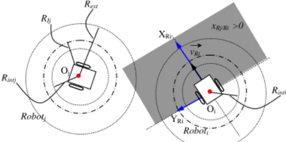
To define ψj(dij), the robot i is surrounded with two
additional virtual circles (cf. Figure 8):
• a circle of radius Rext such that Rext ≥ RIi, (RIi is
the radius of the limit cycle surrounding the robot),
• a circle of radiusRinti such that Rinti< RIi.
The penalty function can then be defined as follows:
ψj(dij) = (dij−Rinti)
(Rext−Rinti) (Rinti< dij < RextandxOj/Ri >0)
0 dij ≤ Rinti
1 otherwise
(13)
wherexOj/Ri is the relative position of the obstaclej in
the relative frame of the roboti (cf. Figure 8). In fact, by
imposingxOj/Ri>0, only the obstacles in front of the robot
i impact its velocity. Robots behind it do not modify it.
When the robot is hindered by M obstacles, its new
velocity noted v0i is then given by
vi0 = vi M
Y
j=1,j6=i
ψj(dij) (14)
whereviis the velocity of the robots given by the Control
Law block without penalty (cf. Equation 9a).
Note that if one hindering obstacle is a robot of the same MRS, the penalty function may cause local minima where two robots (at least) are stopped by each other. In fact, if
Rinti = Rintj anddij ≤ Rinti, then ψj(dij = ψi(dji= 0.
This means thatvi0 = v0j= 0 (cf. Equation 14). To overcome
this minima, and for every couple of robotsk and l such that
(k, l ∈ {1..N }) , radius Rintk andRintl, are attributed such that
|Rintk− Rintl| ≥ ξ
whereξ is the tolerance margin of the robots sensor.
Rintj RIj Rext Robotj Roboti XRi YRi vRi xRj/Ri >0 Oi Oj Rinti
Fig. 8. Virtual circles defining the penalty function ψj(dij).
IV. EXPERIMENTAL RESULTS
Experimentations are made on Khepera III robots. A central camera, at the top of the platform gives positions of all the robots and the obstacles thanks to circular bar codes installed on them. The objective on the long view is to use the local sensors of the robots in order to get a completely decentralized architecture. Experimental results can be illustrated in two paragraph : first, the dynamic obstacle avoidance is shown thanks to a robot joining a static target. In the second paragraph, three robots avoid each other before attaining a dynamic virtual structure.
A. Avoiding a dynamic obstacle
One robot has to reach its static target vT = 0 (cf.
Equation 9a) while avoiding an other robot considered as a dynamic obstacle. The strategy of avoiding dynamic obstacles using the projection of their velocity vector is then shown. Figure 9 shows the robot and the obstacle trajectories. It can be seen that the robot avoids the obstacle by surrounding it behind and attains its final target. Figure 10 shows the variation of the linear velocity of the robot and the distance separating it from the obstacle. It can be seen
that when this distance is d ≤ Rext, the robot decelerates
(its velocity is decreasing) modified by the penalty function
ψ (cf. Equation 13) of the obstacle. When the robot avoids
it, it accelerates again and starts deceleration by reaching the target (cf. Equation 9a).
Dynamic obstacle
Robot Target
(t0) (t1)
Fig. 9. Avoiding a dynamic obstacle.
! " "! # #! $ % # % & % ' () * +, -(2/3156(.129;/0<(9=(0>1(69:90 ! " "! # #! $ %! " ?/*1(),-() * -(7 ! (@1A0 (@/30 (@/30!
Fig. 10. Linear velocity of the robot and distance dRO separating the
robot from the obstacle.
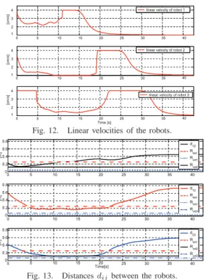
B. Attaining a formation while avoiding collision between the robots
Three robots have to join a triangular virtual structure. They are put in an initial condition such that they must avoid each other using the proposed obstacle avoidance controller (robots of the same system) (cf. Section II-C.3). It is observed that the robots proceed to collision avoidance
before attaining the formation. No conflict was observed since avoidance is done in one direction (counterclockwise). The formation is successfully attained as shown in figure 11 illustrating the trajectories of the three robots. More-over, the penalty function allows to each one deceleration when it approaches other robots offering a bigger time of maneuvering. Figures 12 and 13 represents the variation of the linear velocities and the distances separating each other respectively. By analyzing them, it can be seen how the penalty functions appear when the distances become small
(dij≤ Rext). This explains the diminution of the velocities before reaching the target (cf. Figure 12).
Trajectory of the virtual structure along the circle R3 (t1) R2 (t1) R1 (t1) R1 (t2) R2 (t2) R3 (t2) Virtual structure at moment t0
Fig. 11. Trajectories of the robots attaining the formation.
10 15 20 25 30 35 40 ! " ! c !" # $%&'()*$+(%,-&./$,0$*,1,.$2 3 10 15 20 25 30 35 ! " ! c !" # $%&'()*$+(%,-&./$,0$*,1,.$2 ! " # !ime !" # c !" # $%&'()*$+(%,-&./$,0$*,1,.$3 5 5 5 40 40 35 30 25 20 15 10
Fig. 12. Linear velocities of the robots.
! " "! # #! $ $! % !# !% !& !' () * + (, "# (-./0 (-120" (-120# " # #" $ $! % %" & (, "$ (-./0 (-120" (-120$ $! % %" & 3'())4+ () * + (, #$ (-./0 (-120# (-120$ !# !% !& !' !# !% !& !' () * + " # #" $
Fig. 13. Distances dijbetween the robots.
V. CONCLUSION
A new reactive collision avoidance method, based on limit-cycle approach, is proposed to deal with multi-robot system (MRS). Hence, the control architecture, which allows the navigation in formation of a MRS, is enriched with a more flexible and reliable obstacle avoidance strategies. This
allows to deal with static and dynamic obstacles and permits also to avoid collisions between the robots of the same group. Thus, some conflicts, which were possible when using limit-cycle method for dynamic obstacles, are solved. In addition, the proposed penalty function makes the obstacle avoidance controller more robust against collisions, since it permits to take into account the different local interactions between robots and their environment. Future works will consider the kinematic constraints of the robot while generating the convergence toward the control set-points. The objective is to insure the safety of the robot and the control feasibility.
REFERENCES
[1] P. Fiorini and Z. Shiller. Motion planning in dynamic environments using velocity obstacles. The International Journal of Robotics Research, 17:760–772, 1998.
[2] S. J. Guy, J. Chhugani, C. Kim, N. Satish, M. Lin, D. Manocha, and P. Dubey. Clearpath: Highly parallel collision avoidance for multi-agent simulation. In ACM SIGGRAPH Eurographics symposium on computer animation, 2009.
[3] A. Pongpunwattana and R. Rysdyk. Real-time planning for multiple autonomous vehicles in dynamic uncertain environments. Journal of Aerospace Computing, Information and Communication, 1:580–604, 2004.
[4] O. Khatib. Real time obstacle avoidance for manipulators and mobile robots. International Journal of Robotics Research, 5:90–99, 1986. [5] E. Lalish, K.A. Morgansen, and T. Tsukamaki. Formation tracking
control using virtual structures and deconfliction. IEEE Conference on Decision and Control, 2006.
[6] P. Ogren, E. Fiorelli, and Leonard N. E. Formations with a mission: Stable coordination of vehicle group maneuvers. In 15th International Symposium on Mathematical Theory of Networks and Systems, 2002. [7] S. Mastellone, D.M. Stipanovic, and M.W. Spong. Remote formation control and collision avoidance for multi-agent nonholonomic systems. In IEEE International Conference on Robotics and Automation, pages 1062–1067, 2007.
[8] R. Zapata and P. Lepinay. Reactive behaviors of fast mobile robots. Journal of Robotics Systems, 11:13–20, 1994.
[9] P. Fraisse, R. Zapata, W. Zarrad, and D. Andreu. Remote decentralized control strategy for cooperative mobile robots. Advanced Robotics Journal, Robotics Society of Japan, 19:1027–1040, 2005.
[10] E. Lalish and K.A. Morgansen. Distributed reactive collision avoid-ance. Autonomous Robots, 32, 2012.
[11] A. Benzerrouk, L. Adouane, L. Lequievre, and P. Martinet. Navigation of multi-robot formation in unstructured environment using dynamical virtual structures. IEEE/RSJ International Conference on Intelligent Robots and Systems, 2010.
[12] X. Li, J. Xiao, and Z. Cai. Backstepping based multiple mobile robots formation control. In IEEE International Conference on Intelligent Robots and Systems, pages 887 – 892, 2005.
[13] K. D. Do. Formation tracking control of unicycle-type mobile robots. In IEEE International Conference on Robotics and Automation, pages 527–538, 2007.
[14] T. Balch and R.C. Arkin. Behavior-based formation control for multi-robot teams. IEEE Transactions on Robotics and Autmation, 1999. [15] G. Antonelli, F. Arrichiello, and S. Chiaverini. The nsb control: a
behavior-based approach for multi-robot systems. PALADYN Journal of Behavioral Robotics, 1:48–56, 2010.
[16] H.K. Khalil. Frequency domain analysis of feedback systems (chapter 7). 2002.
[17] D. Kim and J. Kim. A real-time limit-cycle navigation method for fast mobile robots and its application to robot soccer. Robotics and Autonomous Systems, 42:17–30, 2003.
[18] L. Adouane. Orbital obstacle avoidance algorithm for reliable and on-line mobile robot navigation. In 9th Conference on Autonomous Robot Systems and Competitions, May 2009.
[19] J.O. Kim, C.J. Im, H. Shin, K. Y. Yi, and H. G. Lee. A new task-based control architecture for personal robots. International Conference on Intelligent Robots and Systems, 2:1481–1486, 2003.
[20] L. Adouane, A. Benzerrouk, and P. Martinet. Mobile robot navigation in cluttered environment using reactive elliptic trajectories. In 18th IFAC World Congress, 2011.