Feasibility study for conducting a network optimization exercise for the water quality network in lake Winnipeg : existing statistical tools and a first qualitative assessment.

FEASIBILITY STUDY FOR CONDUCTING A NETWORK OPTIMIZATION EXERCISE FOR THE WATER QUALITY NETWORK IN LAKE WINNIPEG:

EXISTING STATISTICAL TOOLS AND A FIRST QUALITATIVE ASSESSMENT

FEASIBILITY STUDY FOR CONDUCTING A NETWORK OPTIMIZATION EXERCISE FOR THE WATER QUALITY NETWORK IN LAKE WINNIPEG: EXISTING STATISTICAL TOOLS AND A FIRST QUALITATIVE ASSESSMENT

By

André St-Hilaire

Taha B.M.J. Ouarda

Bahaa Khalil

Institut national de la recherche scientifique

Centre Eau, Terre et Environnement

(INRS-ETE)

University of Quebec

490 De la Couronne St., Quebec City, G1K 9A9

TABLE OF CONTENT

TABLE OF CONTENT ... III 

LIST OF TABLES ... IV 

LIST OF FIGURES ... V 

1.  INTRODUCTION ... 1 

2.  REVIEW OF EXISTING METHODS ... 2 

2.1VARIABLE SELECTION ... 2 

2.2SELECTION OF STATION LOCATIONS ... 4 

2.3SELECTION OF SAMPLING FREQENCY ... 11 

3.0 FEASIBILITY OF ANALYSIS OF THE CURRENT SAMPLING NETWORK ... 14 

LIST OF TABLES

TABLEAU 1.REPARTITION DU NOMBRE DE RIVIERES INCLUSES DANS L’ETUDE PAR PROVINCE ET PAR REGION

HYDROLOGIQUE AU QUEBEC. ... ERREUR !SIGNET NON DEFINI. TABLEAU 2.INDICES D’ALTÉRATION HYDROLOGIQUE SÉLECTIONNÉS POUR LE QUÉBEC. ... ERREUR !SIGNET NON

DEFINI.

TABLEAU 2.INDICES D’ALTÉRATION HYDROLOGIQUE SÉLECTIONNÉS POUR LE QUÉBEC. ... ERREUR !SIGNET NON DEFINI.

LIST OF FIGURES

FIGURE 1.VARIANCE EXPLIQUÉE PAR CHAQUE COMPOSANTE PRINCIPALE CALCULÉE À PARTIR DES IAH SUR 104

STATIONS HYDROMÉTRIQUES DU QUÉBEC. ... ERREUR !SIGNET NON DEFINI. FIGURE 2.VALEURS DE SATURATION (« LOADINGS ») DES INDICES AVEC LES TROIS PREMIÈRES COMPOSANTES

PRINCIPALES.LES INDICES SONT REPRÉSENTÉES PAR LEUR CATÉGORIE :1(BLEU)=AMPLITUDE,2(TURQUOISE)

=FRÉQUENCE,3(JAUNE)=DURÉE, ET 4(ROUGE)=OCCURRENCE. ... ERREUR !SIGNET NON DEFINI. FIGURE 3.RÉGIONS HYDROLOGIQUES DU QUÉBEC (SOURCE :

HTTP://WWW.CEHQ.GOUV.QC.CA/SUIVIHYDRO/DEFAULT.ASP; ACCÉDÉ LE 22 MARS 2009). ... ERREUR !SIGNET NON DEFINI.

FIGURE 4.SCORES FACTORIELS DES STATIONS HYDROMÉTRIQUES QUÉBÉCOISES, AVEC IDENTIFICATION DES RÉGIONS HYDROLOGIQUES 1 À 12(VOIR FIGURE 3) ... ERREUR !SIGNET NON DEFINI. FIGURE 4.SCORES FACTORIELS DES STATIONS HYDROMÉTRIQUES QUÉBÉCOISES, AVEC IDENTIFICATION DES

SUPERFICIES JAUGÉES ... ERREUR !SIGNET NON DEFINI. FIGURE 6.VALEURS DE SATURATION MIS EN ORDRE POUR SÉLECTIONNER LES INDICES D’ALTÉRATION HYDROLOGIQUE EXPLIQUANT LE PLUS DE VARIANCE. ... ERREUR !SIGNET NON DEFINI. FIGURE 7.VARIANCE EXPLIQUÉE PAR CHAQUE COMPOSANTE PRINCIPALE CALCULÉE À PARTIR DES IAHS SUR 71

STATIONS HYDROMÉTRIQUES DES PROVINCES ATLANTIQUES. ... ERREUR !SIGNET NON DEFINI. FIGURE 8.VALEURS DE SATURATION (« LOADINGS ») DES INDICES AVEC LES TROIS PREMIÈRES COMPOSANTES

PRINCIPALES POUR LES PROVINCES ATLANTIQUES.LES INDICES SONT REPRÉSENTÉES PAR LEUR CATÉGORIE :1

(BLEU)=AMPLITUDE,2(TURQUOISE) =FRÉQUENCE,3(JAUNE)=DURÉE, ET 4(ROUGE)=OCCURRENCE. ... ERREUR !SIGNET NON DEFINI. FIGURE 9SCORES FACTORIELS DES STATIONS HYDROMÉTRIQUES DES PROVINCES ATLANTIQUES,AVEC INDICATION

DES PROVINCES D’APPARTENANCE ... ERREUR !SIGNET NON DEFINI. FIGURE 10.SCORES FACTORIELS DES STATIONS HYDROMÉTRIQUES DES PROVINCES ATLANTIQUES, AVEC

1. INTRODUCTION

Lake Winnipeg is the 11th largest lake in the world (23 750 km2), with a drainage area of 984 200 km2. In recent years, it has been subjected to a number of important anthropogenic stresses, including high nutrient loading that is believed to be the lead cause of important blue-green algal blooms.

This has prompted a major research endeavour on Lake Winnipeg, jointly coordinated by the Lake Winnipeg Research Consortium, Environment Canada, Manitoba Water Stewardship and other federal and provincial departments. In 2003, the Lake Winnipeg Stewardship board was created with a mandate of drafting a management plan. One of the major management objectives is to decrease nitrogen and phosphorous loadings to pre-1970 levels, a target that was set in the Lake Winnipeg Action Plan (http://www.gov.mb.ca/waterstewardship/water_quality/lake_winnipeg/,

Accessed 25 October 2008). This action plan also recognized that research on water quality and the causes of its recent decline is required on Lake Winnipeg.

At the core of the present research effort is the monitoring of lake water quality variables, physical parameters and biota. Limnological surveys have been conducted using a research vessel, the NAMAO. 64 sites were sampled in Lake Winnipeg during these surveys. In Addition, Manitoba Water Stewardship has selected 14 long term stations to sample for long-term trends in a number of physic-chemical variables.

Historical and current sampling effort, albeit variable, provides a unique opportunity for revisiting and potentially optimizing the water quality monitoring network for Lake Winnipeg. This is the main objective of the present project.

This first report aims at providing a brief review of some of the statistical methods that may be used in this project to analyse the adequacy of the current sampling network. In addition, a first, qualitative assessment of the feasibility of implementing some of these statistical methods to the Lake Winnipeg network is provided.

2. REVIEW OF EXISTING METHODS

Khalil and Ouarda (2009) provided an extended literature review of existing statistical methods used to assess and redesign water quality monitoring networks. In this section, only the methods that are deemed useful for this project are reviewed. The reader is referred to Khalil and Ouarda (2009) for a more thorough literature review.

2.1 Variable selection

As stated earlier, variable must first and foremost be selected in accordance with the sampling objectives. Hence, guidelines are often promulgated as thresholds of a certain variable that must not be exceeded. Is such cases, the variable for which the standard is defined must be sampled, unless it can be estimated with sufficient accuracy by a deterministic or statistical model.

Nonetheless, a number of statistical approaches may be used to explore the relationship between variables and quantify the redundancy in multivariate sampling, or alternatively the amount of information gained by sampling additional variables.

The simplest approach is correlation analysis. Pair wise correlations coefficients (r) or coefficient of determinations (r2) can be calculated on concomitant time series of different variables. High correlation values reveal some form of redundancy, i.e. sampling two highly correlated variables does not explain much more variance than sampling only one.

Similarly, linear regressions between variables X and Y can be used:

i

i x

y    (1)

Where α and β are regression coefficients and the εi are estimation errors. If these error terms are

small and the regression model is characterized by high r2 value, than Y can be estimated using X and may not need to be sampled.

Pair wise comparisons may not be suitable when a large number of variables are being sampled. In such cases, multivariate approaches may be deemed more appropriate. One such approach is Principal Component Analysis. PCA aims at reducing the number of variables by transforming them into Principle Components (PC), which are linear combinations of the original variables. In order to achieve this, PCs are constructed with two main criteria: They must be orthogonal (i.e. uncorrelated) and must maximise explained variance of the original dataset.

Thus, the first principal component, PC1 is a linear combination for the original standardized

variables (xi) .



In Equation (1), the variance explained by PC1 is maximized under the following constraint:



Explained variance decreases as principal components are being calculated on residues of the previous PC.

This approach has been used by St-Hilaire et al. (2004) on the Richibucto (N.B.) watershed. More recently, St-Hilaire et al. (2009) have used PCA to select a limited number of pertinent indices of hydrologic alteration (IHAs) out of an initial suite of 88 indices. Figure 1 shows the projection of loadings (correlation between original variables and the PC) in PC1-PC2 space for

88 indices. The IHAs, which are various descriptive statistics of the hydrograph (monthly or annual means, timing and duration of low flows, etc.) calculated from time series of daily flows, were divided in four categories related to the characteristic of the hydrograph that they describe : Amplitude (dark blue), Timing (red), Frequency (light blue) and duration (orange).

Figure 1 shows evidence of clustering of some of the IHAs. These clusters indicate that the correlation between IAHs within this group and the PCs are roughly equivalent. Hence, it may be possible to select one or two IAHs from the cluster as a representative of the group.

Figure 1. Loadings of Indices of hydrological Alteration in Principal Component space (from St-Hilaire et al., 2009).

In addition to selecting variables within cluster, an additional selection criterion can by the loading value. Figure 2 shows the sorted loading values for the 88 IAHs presented in Figure 1. An objective criterion can be used to select IHAs from this graph. For instance, variables with loadings >|0.15| may be selected. Alternatively, a fixed number of IHAs with the highest loadings could be selected.

Figure 2. Sorted loadings for the 88 IHAs of Figure 1 (from St-Hilaire et al., 2009).

The relation between different variables is not necessarily linear and it may not be captured by linear methods. Recently, Artificial Neural Networks (ANNs) have gained popularity in

hydrology and other scientific disciplines because of their ability to model such non-linear relationships.

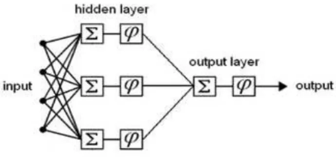
ANNs (Figure 3) are computational models that consist of a set of processing elements (neurons) and connections between them, as well as training algorithm (Tambe et al., 1996). A suitably trained neural network is able to generalize from the training set, and provide reasonably accurate predictions when presented with new inputs that were not part of the original training set. There are different types of neural networks, which differ from one another in architecture and training algorithms. The multi layer feed-forward neural network is one of the most widely used ANN (Brosse et al, 1999). It has been proven that these networks with at least one hidden layer can map inputs and outputs related by nonlinear function. This class of ANNs consists of three neural layers: an input layer, one or more hidden layers, and an output layer (Figure 3). The input layer is made up of predictor variables nodes (neurons) and a bias node used during neural network training. The hidden layer is the location where the neural network is trained. The training consists in modifying the weights until adequate mapping between input and outputs is obtained.

Figure 3. Schematic of a feed-forward Artificial Neural Network.

Khalil et al. (2007) successfully used ANNs to investigate the interrelation of water quality variables in a drainage system located in the Nile Delta (Egypt).

2.2 Selection of station locations

Station location can be selected for each water quality variable of interest individually or for a group of variables using multivariate approaches. As for variable selection, correlation and regression analyses can be used to assess the redundancy between two stations. Multivariate linear regression can be used as a tool to assess one station (dependant variable Y in Equation 1), against all the others (independent variables X). In such cases, Tirsh and Male (1984) proposed to use the coefficient of determination (r2) as a criterion to determine whether a specific station location is required.

An alternative use of linear regression consists in calculating the information content of the mean for two stations (X and Y) with unequal sample sizes (n1i+n2 and n1 respectively)

Site X : x , x , ..., x , x_{1 2 n n 1}, x_{n 2}, ..., x_n n 2

1 1 1 1

Site Y : y , y , ..., y_{1 2 n}

1

Using the concomitant portion of the sample, Y values for the n2 time steps can be estimated

from X using Equation 1. The mean of the augmented Y series can be estimated as:





where y₁ is the mean of the yi observations during the n1 period and x1, x2 are the means of the xi observations during periods n1 and n2 respectively. The variance of the estimated mean is :

 

Where _y2 is the variance of Y and  is the correlation coefficient between X and Y. The bracketed term is called the information content. It can be shown that in order to improve the estimate of the mean by augmenting the series using the regression, the following criterion must





 n₁2 1 2 (6)

Hence, the information content of each station can be estimated from correlated stations using this criterion and by subdividing the time series in order to use equations (4), (5) and (6).

On method that has been used relatively frequency for station location analysis is based on the concept of entropy (Harmancioglu et al., 1999), which measures the amount of degree of uncertainty in trans-information (redundancy between measurements at different locations. For a network of n locations, characterized by a covariance matrix C, the joint entropy is calculated for different classes of distances x by:

( ) ( / 2) ln 2 0.5 ln ( / 2) ln( )

H x  n  C  n n x (7)

Different network configurations can be designed and a value of joint entropy can be calculated for each one, thereby permitting a quantitative comparison. Alternatively, marginal entropy for a given station can be calculated for n=1 and replacing the covariance matrix by variance. Entropy must be calculated for each water quality variable separately.

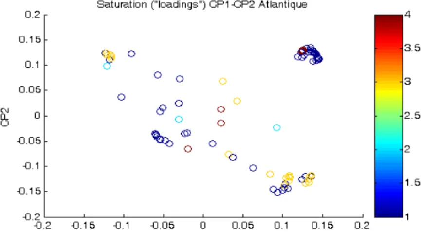
Multivariate approaches such as PCA can also be used to provide information on station location and potential redundancy in information. Instead of projecting loadings of variables in the PC space, stations scores (estimation of the PC values for each station) can be projected in the same space. Using the same example on IHAs provided by St-Hilaire et al. (2009), PC scores were projected for 71 stations in Atlantic Canada (Figure 4). Station numbers have been replaced by the Province of origin, to highlight geographical proximity. In this example, Figure 4 shows that a number of stations in Prince-Edward Island (PEI) and Newfoundland (NF), as well as two from New Brunswick (NB) and Nova Scotia (NS) stand out of the main cluster. It could be therefore argued that these stations have a distinct hydrological signature and should be sampled.

Figure 4. Projections of PCA scores for Indices of Hydrologic Alteration in Principal Component Space.

Other multivariate approaches such as Cluster Analysis (Johnson, 1998), Canonical Correlation Analysis (Guillemette et al., 2008) and Discrimant Analysis (Rao, 1973) could also be used for station selection.

Geostatistical approaches have also been used to rationalize networks. A popular spatial interpolation technique called kriging has been used by St-Hilaire et al. (2003) to investigate the increase of interpolation error as a function of network density. Kriging can be performed in two main steps.

The first one consists in calculating an experimental semi-variogram and fitting a theoretical model to it. The semi variogram is an estimation of the dissimilarity between measurements of a given variable as a function of separation distance:







Where N(h)is the number of data pairs at a separation distance h which have an observed values z(x). A theoretical model is then fitted to the experimental semi-variogram such as spherical, exponential, or Gaussian functions with three parameters: the nugget effect (C0), the

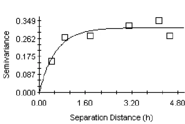
sill (c) and the range (a) (Figure 5). The nugget effect describes the occurrence of discontinuity at the origin of the semi-variogram that may be caused by dissimilar sample values at short inter-station distances. The sill is the plateau reached by the variogram beyond a certain inter-inter-station distance. This plateau indicates a value of semi-variance that is a threshold beyond which there is essentially no spatial structure in the data. Finally, the range represents the inter-station distance over which the observed values are correlated. Variographic analysis can be used on its own to determine a minimum inter station distance that guarantees independence. This distance would be equivalent to the range.

Figure 6. An example of experimental (squares) and theoretical (line) semi-variogram (from Guillemette et al., 2009).

The second step is to perform an interpolation of the selected variable. For any point in the study area, this interpolation will be performed as a weighted sum of the measured values:



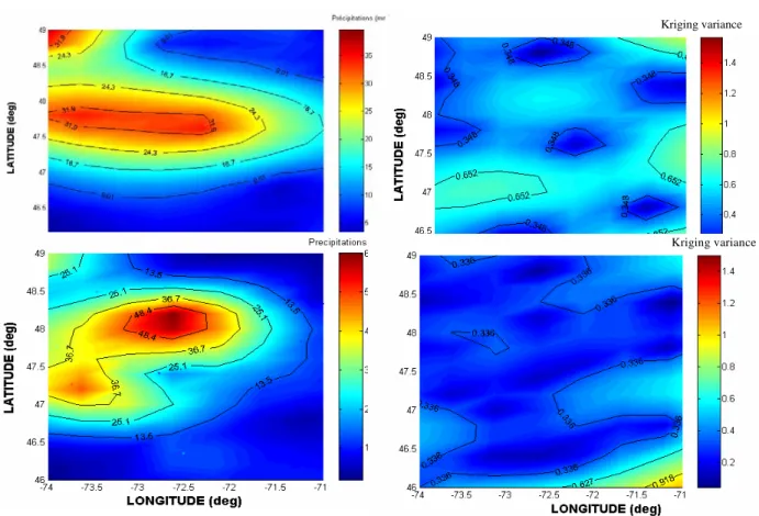
Where _i are the weights of the estimator that minimize the variance of the estimation errors. By using the spatial structure defined by the theoretical semi-variogram, a kriging system of linear equations combining neighbouring information can be defined and the weights can be estimated. Kriging can thus be used to estimate the water quality variable throughout the study area, using the existing network. Kriging variance, which is a measure of the estimation errors, can also be mapped throughout the area. St-Hilaire et al., (2002) used this approach to assess the increase in error in estimated precipitation as a function of network density in central Québec. In Figure 8, the upper panel shows the interpolated precipitations for a rain event in the study area (8 June 1999) on the left, and its associated error (kriging variance) on the right for a network of 27 stations. The lower panel shows the interpolated values and variance for a network of 48 stations. Subsequently, the study area was divided in sub regions of 20 km2. The kriging variance was calculated for each square and the number of sampling stations within each square was counted. Boxplots of kriging variance as a function of station density were then plotted for the two network scenarios. Figure 8 shows the reduction of variance when the interpolation is performed with 48 stations (left panel), vs. 27 stations (right panel). Hence, different network configurations can be tested. However, the approach is limited to rationalization. The maximum number of stations that can be considered is the existing network.

Figure 7. Interpolated precipitations and kriging variance for a rain event in Québec (from St-Hilaire et al., 2003).

Figure 8. Kriging variance as a function of the number of stations per area (20 km2) for

network of 27 stations (left) and a network of 48 stations (right; from St-Hilaire et al., Kriging variance

2.3 Selection of sampling frequency

Frequency of data collection is another important parameter that should ideally be optimized in a monitoring program. Some of the approaches that may be used in the present project include methods that deal with means and trends in time series and geostatistical approaches.

A number of statistical tests exist to establish if there is a significant trend or autocorrelation in the time series. Such approaches are dubbed “effective sample methods” because they seek to establish a sampling frequency that maintain independence (or avoid autocorrelation) of the sample points. The approach used by Lachance et al., (1989) remains appealing because of its relative simplicity. Given a time series of a variable sampled n times per year, one can calculate an autocorrelation function (ACF), which is simply the correlation between the variable at time t and the same variable at time t-k, where k is called the lag. The effective sample size n* can be calculated using the following equation:

1 2 1 1 1 2 ( ) * n k k n k ACF n n n    



It should be noted that equation (7) should be applied on de-trended data.

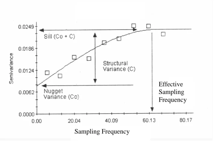
One other potential approach is to use the variogram defined in equation (7), but replacing inter-station distance by time lag. The lag at which the sill is reached is the time step beyond which there is no autocorrelation in the data and hence can be used as the frequency of sampling that guarantees independence (Figure 9).

Figure 8. Temporal sampling semi-variogram to determine the effective sampling frequency.

Sampling Frequency

Effective

Sampling

Frequency

3.0 FEASIBILITY OF ANALYSIS OF THE CURRENT

SAMPLING NETWORK

The various statistical methods described in the previous section are a sub sample of the approaches available in the literature. They are described in this report because it was felt by the authors that they may be applicable to assist in assessing and perhaps providing input in the redesign of the monitoring network, should it be required.

Presently, the main monitoring network consists of 64 stations visited three times per year on the lake (Figure 10). Fourteen stations are sampled more intensively (i.e. more variables, longer time series) by Manitoba Water Stewardship. IN addition other existing data include:

 Limnological surveys during the 1970s that included 70 sites  65 sites revisited in the 1990s

 Fixed moorings to sample current (ADCP), and some water quality variables (e.g. DO, conductivity, temperature at several depths) at eight locations throughout the lake (LWRC, 2008).

These additional data may potentially be used in the analysis of the network, if they become available. The initial emphasis of the project will be on variables and station location selection. These analyses could initially focus on the current sampling network. Historical data may potentially be used, but there is a risk that non-stationnarities of a number of variables (i.e. difference in mean values of variables sampled decades ago and now) that may be caused by lake conditions, but also by modifications in the sampling procedure may preclude their usage.

Sampling frequency may also be problematic. In order to investigate effective sampling frequency, relatively long time series are required. The fixed moorings deployed in the lake during the ice-free season probably offer the best data set to investigate optimal sampling frequency. This means that at the onset, only a few variables can be analysed to define the effective frequency of measurements.

Figure 10. Monitoring stations of Lake Winnipeg (Source, Lake Winnipeg Research Consortium, 2007)

The existing GIS database offers the possibility of including physiographic and morphometric information as independent variables that may assist in assessing the suitability of the current network. Basin and lake characteristics should be included in the decision making process that may lead to a re-design of the network. Variables such as depth at stations, proximity to lake tributaries, fetch, etc. can be taken into account in multivariate approaches such as neural networks and PCA or Canonical Correlation Analysis (CCA, see Guillemette et al., 2008). A more informative assessment can thus be made.

3. CONCLUSION

Lake Winnipeg is subjected to anthropogenic stresses and a monitoring effort is required to define indicators of ecosystem health and sustainability. In order to define indicators that are truly significant of this large ecosystem, the sampling design must be revisited and assessed against objective criteria. The present report summarized some of the statistical tools available that can assist in selecting the variables to be sampled, the sampling locations and the frequency at which the measurements should be made.

At the onset, it appears that a number of the approaches described herein may be applicable in the context of the Lake Winnipeg current sampling program. Inclusion of historical data in the analysis may be possible, but will have to be further investigated in light of potential discontinuities in the sampling protocol and other sources of non stationarity.

REFERENCES

Brosse S., Guégan J.F., Lek S. 1999. The use of artificial neural networks to assess fish abundance and spatial occupancy in the littoral zone of a mesotrophic lake. Ecological Modelling

120: 299-311.

Guillemette, N. A. St-Hilaire, T.B.M.J. Ouarda, N. Bergeron, E. Rrobichaud, L. bilodeau. 2009. Feasibility study of a geostatistical modelling of monthly maximum s stream temperatures in multivariate space. Journal of hydrology 364:1-12

Harmancioglu, N.B., Fistikoglu, O., Ozkul, S.D. Singh, V.P. and Alpaslan, M.N. 1999. Water quality Monitoring Network Design. Kluwer Academinnc Publishers, Dordrecht, The nether lands, 290 p.

Khalil, B.M., AA George, H. Karaman, and A. EL-Sayed. 2007. Application of Artificial Neural Networks for the prediction of Water Quality variables in the Nile Delta. NAWQAM final conference. “Egypt paradigm in integrated water resources management”, Sharm-Elsheikh, Egypt, 59-69.

Khalil, B.M., T.B.M.J. Ouarda. 2008. Statistical Approaches used to assess and redesign surface water quality monitoring networks. To be submitted.

Johnson, D.E. (1998). Applied multivariate Methods for Data Analysts. Pacific Grove, CA, Duxburry Press, 592 P.

Lachance, M., B. Bobéee, J. Haemmerli. 1989. Methodology for the planning and operation of a qater quality network with temporal and spatial objectives: application to acid lakes in Quebec, In R.C. Ward, J.C. Loftis and G.M. McBride (eds). Proceedings, International Symposium on the Design of Water Quality Information Systems, Fort Collins, CSU Information Series no 61:145-162.

Lake Winnipeg Research COnsurtium. 2008. The Lake Winnipeg Research Consortium Inc. Research, Education and Outreach Activities April 1, 2007 – March 31, 2008. 24 p.

Matalas N.C. and W.B. Langbein (1962). Information content of the mean. Journal of

Geophysical Research, 67(9): 3441-3448.

Rao, C.R. 1973. Linear statistical inference and its Applications, Second Edition, New York, John Wiley and Sons, 625 p.

St-Hilaire, A., Ouarda, T.B.M.J., Lachance, M., Bobée, B., Gaudet, J. and C. Gignac 2003. Assessment of the impact of meteorological network density on the estimation of precipitation and runoff: A case study. Hydrological Processes 17(10):3561-3580

St-Hilaire, A. G. Brun, S.C. Courtenay, T.B.M.J. Ouarda, A.D. Boghen et B. Bobée. 2004. Multivariate analysis of water quality in the Richibucto (N.B.) Drainage Basin. Journal of

American Water Resources Association 40(3):691-703

St-Hilaire, A., A. Daigle, D. Beveridge, L. Benyahya, D. Caissie. 2009. Analyse multivariée des indices d’altération hydrologique de l’est du canada. INRS-ETE Research Report, 29 p.

Tambe SS, Kulkarni BD, Deshpande PB. 1996. Elements of Artificial Neural Networks with Selected Applications in Chemical Engineering, and Chemical and Biological Sciences. Simulation and Advanced Controls, Inc: Louisville, Kentucky.

Tirsch, F.S. and J.W. Male. 1984. River basin water quality monitoring network design: options for reaching water quality goals, in T.M. Schad (ed.) Proceedings of the 20th Annual Conference of the AWRA: 149-156.