Modélisation régionale de type débit-durée-fréquence (QdF) des évènements de crues printanières dans un cadre non stationnaire.

Université du Québec INRS-Eau, Terre et Environnement

Modélisation régionale de type débit-durée-fréquence (QdF) des événements de crues printanières dans un cadre non stationnaire

Par

V éronique Jourdain

Mémoire présenté pour l'obtention

du grade de Maître ès sciences (M. Sc.) en sciences de l'eau

Jury d'évaluation Président du jury et examinateur interne Directeur de recherche

Examinateur externe

28 décembre 2006

© Droits réservés de Véronique Jourdain, 2006

Karem Chokmani, INRS-ETE Taha Ouarda, INRS-ETE Musandji Fuamba, École Polytechnique de Montréal, Département des génies civil, géologique et des mines

AVANT-PROPOS

Ce mémoire par article comporte d'abord, en section 1, une synthèse qui fait état de la problématique et de la pertinence de mon sujet de recherche, ainsi que de la contribution que j'ai apportée à ce travail de recherche. Sont aussi présentés les principaux résultats obtenus ainsi que les conclusions et recommandations. De plus amples détails concernant ces travaux de recherche sont présentés dans l'article soumis au journal Hydrological Processes. L'article est présenté à la section 2 du présent document.

Le titre et les auteurs de l'article soumis sont les suivants:

Titre:

Auteurs:

Non-stationary regional QdF analysis: An application to the estimation of spring flood quantiles in southern Ontario (Canada) and New England (USA)

Véronique Jourdain, Taha B.M.J. Ouarda, Juraj M. Cunderlik, Salaheddine El Adlouni.

Les contributions des auteurs sont divisées comme suit:

Véronique Jourdain:

Taha B.M.J. Ouarda :

Juraj Cunderlik :

Contribution à la conception du projet et à l'élaboration de la méthodologie, Construction des bases de données hydrologiques, météorologiques et physiographiques, Programmation informatique, interprétation des résultats, rédaction de l'article.

Contribution à la conception du projet, à l'élaboration de la méthodologie, à l'interprétation des résultats et à la rédaction de l'article.

Contribution à la rédaction de l'article, aide pour la résolution de problèmes lors de la programmation informatique du modèle proposé.

Salaheddine El Adlouni: Contribution pour l'analyse fréquentielle locale non stationnaire.

RÉSUMÉ

L'analyse débit-durée-fréquence (notée QdF) tient compte de la variabilité temporelle des crues. Ainsi, les modèles régionaux de type QdF permettent l'estimation des quantiles de crues à des sites non jaugés non seulement en fonction de la période de retour, mais également en fonction de la durée de la crue. Ces modèles QdF ont été surtout développés dans un cadre stationnaire, c'est-à-dire lorsque aucune tendance n'est présente dans les séries hydrologiques. Plusieurs études indiquent des changements temporels importants des caractéristiques statistiques des débits de crue. En effet, des tendances statistiques significatives sont de plus en plus observées et, dans ce cas, les séries hydrologiques ne respectent plus l 'hypothèse de stationnarité sur laquelle reposent de nombreux modèles QdF. De nouvelles méthodes d'estimation des quantiles de crues tenant compte de la présence de non-stationnarité dans les séries hydrologiques doivent donc être développées. Le modèle proposé dans ce mémoire est une approche régionale non stationnaire de type QdF basée sur les voisinages hydrologiques définis par l'analyse canonique des corrélations (notée ACC). Un ensemble de 22 stations hydrométriques situées au sud de l'Ontario (Canada) ainsi qu'en Nouvelle-Angleterre (États-Unis) a été utilisé pour évaluer la performance de l'approche proposée. Une procédure de type « jackknife » a été employée pour évaluer la performance de la méthode pour l'estimation des quantiles de crues par la modélisation QdF. Les résultats basés sur les voisinages hydrologiques ont été comparés à ceux obtenus à partir d'un scénario où l'information disponible dans toutes les stations hydrométriques est employée pour l'analyse. Par ailleurs, afin d'évaluer l'erreur faite en employant un modèle QdF stationnaire en présence de non-stationnarité dans les séries hydrologiques, les résultats obtenus à partir d'une approche QdF stationnaire ont été comparés à ceux obtenus à partir du modèle proposé. Pour les stations hydrométriques à l'étude, on conclut finalement à la supériorité du modèle QdF non stationnaire basé sur les voisinages hydrologiques. En effet, la combinaison ACC et modélisation QdF non stationnaire, c'est-à-dire l'approche proposée, permet d'obtenir, en présence de non-stationnarité, des estimations des

quantilesde crue de plus grande 9ualité.

~2

n .

.

l~~dA

_____

C

~~~~

REMERCIEMENTS

En préambule à ce mémoire, Je souhaite adresser ici tous mes remerciements aux personnes qui m'ont apporté leur aide et qui ont ainsi contribué à l'élaboration de ce mémoire.

Tout d'abord Monsieur Taha Ouarda, directeur de recherche, pour l'aide, le support et le temps qu'il m'a consacrés. Merci aussi à Martin Leclerc, étudiant à la maîtrise à l'INRS-ETE, avec qui j'ai eu le plaisir de collaborer tout au long de ma maîtrise.

Enfin, j'adresse mes plus sincères remerciements à tous mes proches et amis qui m'ont toujours soutenue et encouragée au cours de la réalisation de ce mémoire.

TABLE DES MATIÈRES

Avant-Propos ... iii Résumé ... iv Remerciements ... v Section 1 : Synthèse ... 1 1. Introduction ... 2

2. Situation de la contribution de l'étudiant ... .4

3. Contribution de l'étudiant ... 6

4. Résultats et conclusions ... 9

5. Bibliographie ... 11

Section 2: Article scientifique ... 14

1. Non-stationary regional QdF analysis: an application to the estimation of spring flood quantiles in a set of catchments located in Southem Ontario (Canada) and New England (USA) 16

1. Introduction 18

2. Literature review of QdF and non-stationary models 19

3. Theoretical background 21

3.1 Canonical correlation analysis 21

3.2 Regional QdF modeling 24

3.2.1 Stationary QdF approach 24

3.2.2 Non-stationary QdF approach 25

4. Proposed non-stationary regional QdF model 26

5. Application 29 5.1 Studyarea 29 5.2 Methodology 30 5.3 Results 32 6. Conclusions 34 7. Acknowledgment 36 8. References 37

j

j

j

j

j

j

j

j

j

j

j

j

j

j

j

j

j

j

j

j

j

j

j

j

j

j

j

j

j

j

j

j

j

j

j

j

j

1.

Introduction

Mes travaux de recherche, rapportés dans l'article présenté à la section 2, concernent les modèles débit-durée-fréquence (noté QdF). Ces modèles permettent de représenter les quantiles de crues non seulement en fonction de la période de retour, mais aussi de la durée de la crue. Pour la prévention des inondations ou la construction d'ouvrages sur les cours d'eau, il est en effet important d'évaluer les crues par leur importance en terme de débit, mais aussi par leur variabilité temporelle. Cependant, les méthodes d'estimation des quanti les de crues souvent utilisées ignorent ces variables importantes que sont la durée et la variabilité de la crue.

Par ailleurs, la perception d'un climat changeant et de plus en plus variable est maintenant généralement admise. Ce climat changeant a possiblement un impact sur les processus hydrologiques. Au cours de la dernière décennie, plusieurs études rapportent des changements temporels cruciaux des caractéristiques du régime hydrologique des cours d'eau (Lins et Slack, 1999; Zhang et al., 2001; McCabe et Wolock, 2002; Douglas et al.,

2000). En présence de non-stationnarité dans les séries hydrologiques, les caractéristiques statistiques d'une série chronologique, telles que la moyenne et la variance, varient dans le temps. Dans ce cas, les méthodes traditionnellement utilisées, c'est-à-dire reposant sur l'hypothèse de stationnarité, ne peuvent plus être utilisées avec confiance. En effet, en ignorant la présence de tendances négatives ou positives, ces méthodes peuvent conduire à de fortes surestimations ou sous-estimations. Ainsi, il devient de plus en plus important de développer des modèles permettant l'estimation des quantiles de crues en présence de non-stationnarité.

Par ailleurs, l'estimation des débits de crues à des sites où l'on dispose de peu ou même d'aucune information hydrologique s'avère souvent nécessaire. En effet, l'aménagement des cours d'eau, la gestion des réservoirs, la caractérisation de l'écoulement d'un bassin versant et l'évaluation des risques et dégâts nécessitent la connaissance du régime hydrologique du cours d'eau à des sites où l'on ne dispose pas de système de mesure du débit. À cette fin, on peut avoir recours à des méthodes de régionalisation des débits

extrêmes qui permettent d'utiliser les données disponibles à d'autres sites semblables, selon certains critères, au site non jaugé. La régionalisation comporte deux étapes principales: la détermination des régions homogènes et l'estimation régionale. La détermination des régions homogènes peut se faire de diverses façons. Des régions géographiques correspondant à un regroupement de stations hydrométriques contiguës ou non contiguës peuvent être utilisées. On utilise aussi des méthodes basées sur des régions de type voisinage définies, par exemple, par l'analyse canonique des corrélations (notée ACC) (Ouarda et al., 2001). Ce type d'approche permet de définir pour chaque site d'intérêt un voisinage hydrologique qui lui est propre, c'est-à-dire un ensemble de stations hydrologiquement similaires au site d'intérêt.

L'objectif principal de mon projet de recherche visait donc le développement d'un modèle régional QdF non stationnaire pour l'estimation des quantiles de crues à des sites non jaugés. Plus précisément, les travaux de recherche rapportés dans l'article présenté dans ce mémoire présentent une approche régionale non stationnaire de type QdF basée sur des voisinages hydrologiques. Pour l'identification des voisinages hydrologiques, la méthode de l' ACC a été utilisée. En pratique, en présence ou non de non-stationnarité, la modélisation QdF non stationnaire reste peu utilisée. Donc, pour valider la performance du modèle non stationnaire proposé, le projet de recherche visait aussi l'évaluation de l'erreur obtenue par l'utilisation d'un modèle QdF stationnaire en présence de non-stationnarité dans la série hydrologique. Pour atteindre les objectifs de recherche fixés, des données hydrologiques réelles provenant d'un ensemble de stations hydrométriques situées au sud de l'Ontario (Canada) ainsi qu'en Nouvelle-Angleterre (États-Unis) ont été utilisées.

2.

Situation de la contribution de l'étudiant

Pour en arriver au développement du modèle QdF non stationnaire proposé, différentes approches tenant compte de la variabilité temporelle des crues ont tout d'abord été proposées. Parmi celles-là, on compte l'analyse « Pointe-volume» (Ashkar, 1980) ainsi que l'approche « volume au-dessus d'un certain seuil» (Cunnane, 1989). Ensuite, des formes préliminaires des modèles QdF ont été proposées. Ces modèles ont tout d'abord été développés pour l'estimation locale des quantiles telle que la modélisation QdF proposée par Galéa et Prudhomme (1997). Ensuite, Javelle et al. (1999) ont proposé un

modèle convergent et continu de type QdF. Cette approche est basée sur les propriétés d'invariance d'échelle des distributions de crue. Elle a été appliquée en France (Javelle et al., 2000), en Guadeloupe (Galéa et Javelle, 2000), au Burkina Faso (Mar et al., 2002)

ainsi qu'en Roumanie (Mic et al., 2002).

Par ailleurs, lorsqu'un site est non jaugé ou partiellement jaugé, des techniques d'estimation régionale doivent être utilisées. La modélisation QdF régionale a été introduite en France par Galéa et Sourisseau (1997). Ultérieurement, la modélisation QdF a été combinée à la méthode de l'indice de crue (Dalrymple, 1960). Cette dernière approche, proposée par Javelle et al. (2002), a été appliquée à 150 stations situées dans la

province de Québec (Canada) ainsi qu'à un ensemble de stations situées dans les provinces du Québec et de l'Ontario (Canada) (Javelle et al., 2003). Inspirés par cette

approche régionale, Cunderlik et Ouarda (2006) ont proposé un modèle QdF non stationnaire.

Cette approche QdF non stationnaire est d'une grande importance. En effet, au cours des dernières années, de nombreuses études ont rapporté la présence de tendances significatives dans les séries hydrologiques (Lins et Slack, 1999; Zhang et al., 2001;

McCabe et Wolock, 2002; Douglas et al., 2000). Cela implique que les méthodes

traditionnelles, c'est-à-dire les méthodes ayant comme hypothèse de base la stationnarité des séries, ne peuvent plus être appliquées avec confiance. L'approche QdF régionale non stationnaire développée par Cunderlik et Ouarda (2006) permet l'estimation régionale des

quantiles de crues. Elle considère que les deux premiers moments de la série ne sont pas stationnaires, c'est-à-dire le paramètre de position et le paramètre d'échelle, ainsi que dans un paramètre caractérisant la dynamique des crues. Elle a été appliquée à un ensemble de 8 stations hydrométriques situées dans la province du Québec, Canada.

C'est à partir de cette dernière approche QdF régionale non stationnaire qu'a été développée, au cours de mes travaux de maîtrise, une approche régionale QdF non stationnaire basée sur des voisinages hydrologiques déterminés par l'ACC. L'ACC a déjà fait ses preuves dans un cadre stationnaire (Ouarda et al., 2001; Girard et al., 2000), mais n'a toujours pas été combinée à un modèle non stationnaire et, de surcroît, à un modèle QdF non stationnaire. Ma contribution par ce travail de recherche constitue donc en un avancement des travaux de modélisation régionale non stationnaire, plus particulièrement dans le cas de la modélisation QdF. En effet, l'approche régionale proposée permet l'estimation des quantiles de crues à n'importe quel site non jaugé en se basant sur un voisinage hydrologique. De plus, elle tient compte de la présence de non-stationnarité dans les séries hydrologiques et permet aussi, par la modélisation QdF, de prendre en considération la variabilité temporelle des crues.

3.

Contribution de ['étudiant

Préalablement à mes premiers travaux de recherche, j'ai effectué à la session d'automne 2004 ainsi qu'à l'hiver 2005, une revue de la littérature concernant les modèles QdF ainsi que les modèles non stationnaires. Les résultats de cette recherche sont présentés dans la section « Literature review of QdF and non-stationary models» de l'article présenté à la section 2 du présent document. J'ai ensuite travaillé au développement et à l'amélioration du modèle QdF régional non stationnaire dès la fin de l'hiver 2005. J'ai effectué la validation des résultats obtenus par ce modèle à la fin de l'hiver 2006 ainsi qu'au printemps 2006. Le modèle a donc été finalisé au printemps 2006. Il est présenté en détails, sous sa version finale, à la section 4 de l'article, section intitulée « Proposed non-stationary regional QdF model ».

Pour tester l'approche proposée, j'ai élaboré et retenu, avec la contribution de mon directeur, une méthodologie adaptée à mes objectifs de recherche. Ce modèle a été testé à partir de données réelles. Les stations hydrométriques utilisées pour tester le modèle sont situées au sud de l'Ontario (Canada) ainsi qu'en Nouvelle-Angleterre (États-Unis). La localisation géographique des stations utilisées est présentée à la Figure 1 de la section 5.1 de l'article (intitulée « Study Area »). Vu le territoire à l'étude, c'est-à-dire un territoire touché par des hivers froids et donc une fonte importante de la neige au printemps, j'ai convenu avec mon directeur de recherche de me concentrer sur l'étude des crues printanières. Les bases de données hydrométriques, météorologiques et physiographiques décrivant les caractéristiques des bassins versants du sud-est du Canada et du nord-est des États-Unis ont été développées conjointement par moi-même avec la collaboration de Martin Leclerc, étudiant à la maîtrise en sciences de l'eau à l'INRS, centre Eau, Terre et Environnement. Martin Leclerc et moi avons travaillé en équipe pour cette étape de nos projets de maîtrise, car ces derniers nécessitaient tous deux l'utilisation d'une telle base de données. Les tâches ont été divisées comme suit: je me suis occupée de recueillir et de traiter les données hydrométriques et physiographiques pour les bassins versants du sud-est du Canada et Martin Leclerc a fait de même pour les bassins versants du nord-est des États-Unis. Martin Leclerc s'est aussi chargé de recueillir

et de traiter les données météorologiques pour l'ensemble du territoire à l'étude. De plus, il a effectué le travail permettant d'associer chacune des stations hydrométriques utilisées à la station météorologique appropriée. La construction des séries de crues printanières, c'est-à-dire l'extraction des maximums printaniers à partir des séries de débits maximums journaliers, a aussi été effectuée conjointement par Martin Leclerc et moi-même. Puisque nos projets de recherche concernent le développement de modèles non stationnaires, des séries de crues printanières présentant une tendance sur une période d'enregistrement donnée ont été considérées. Pour en faire l'identification, Martin Leclerc et moi avons aussi effectué la programmation ainsi que l'application d'un test permettant de vérifier l'hypothèse de stationnarité des séries. Le test utilisé est une version modifiée du test de Mann-Kendall (Yue et Pilon, 2003). L'ensemble des 22 stations hydrométriques sélectionnées présente donc une tendance négative sur la période 1974 à 2003. Tous ces éléments et principales étapes de ces travaux sont résumés à la section 5.1 de l'article (intitulée « Study Area »).

Afin de valider les résultats obtenus par le modèle QdF régional non stationnaire, des estimations locales ont été obtenues pour chaque station hydrométrique considérée. J'ai donc tout d'abord obtenu ces estimations par analyse fréquentielle locale stationnaire à l'aide d'une procédure automatisée développée par l'équipe de la chaire de recherche du Canada en estimation des variables hydrologiques. J'ai d'ailleurs modifié cette procédure pour répondre aux besoins spécifiques de mon projet. De plus, j'ai aussi obtenu les estimations des quantiles locaux par analyse fréquentielle locale non stationnaire. Plus particulièrement, la distribution OEV (Oeneralized Extreme Values) adaptée au cadre non stationnaire (El Adlouni et al., 2005) a été utilisée. Salaheddine El Adlouni, associé de

recherche dans l'équipe de la chaire de recherche du Canada en estimation des variables hydrologiques, m'a aidé en me fournissant les programmes informatiques permettant l'ajustement des paramètres de cette distribution. J'ai adapté ces programmes dans le but qu'ils répondent à mes besoins spécifiques. Toujours en ce qui concerne l'analyse fréquentielle locale, j'ai choisi les périodes de retour à considérer avec l'aide de mon directeur, Taha Ouarda. Les périodes de retour choisies sont T=5, 100 ans. De plus, avec

évaluer la performance du modèle proposé. Cette procédure est décrite à la section 5.2 de l'article. J'ai ensuite obtenu les résultats concernant l'identification des voisinages hydrologiques par l'ACC. À des fins comparatives, ces voisinages hydrologiques ont été obtenus sur la base des quantiles locaux stationnaires ainsi que sur celle des quantiles locaux non stationnaires. L'ACC est décrite en détails dans l'article à la section 3.1. Pour la détermination des voisinages hydrologiques par ACC, un programme informatique préparé antérieurement par des membres de l'équipe de la chaire de recherche du Canada en estimation des variables hydrologiques a été utilisé. Afin d'évaluer la performance de la méthode basée sur les voisinages hydrologiques, j'ai convenu avec mon directeur de recherche de comparer ces résultats à ceux obtenus en considérant comme région homogène, pour chacune des stations, l'ensemble des stations hydrométriques restantes de la base de données. Pour obtenir les estimations régionales non stationnaires de type QdF basées sur les voisinages hydrologiques, j'ai entièrement programmé la procédure moi-même à l'aide du logiciel MATLAB (The MathWorks, Inc., 2005). Juraj Cunderlik m'a aidée lors de la programmation. Pour l'analyse QdF, j'ai choisi, avec l'aide de mon directeur, les durées à considérer, c'est-à-dire d = 1, 5, 7, 9, 13, 15 jours. J'ai obtenu moi-même tous les résultats présentés dans l'article à la section 5.2 de l'article et j'ai aussi produit toutes les figures ainsi que tous les tableaux. De plus, à des fins de comparaisons, la modélisation QdF stationnaire a aussi été utilisée. J'ai entièrement programmé cette méthode et j'en ai aussi tiré tous les résultats qui m'étaient utiles pour mon projet de recherche. Pour l'évaluation des résultats, j'ai choisi d'utiliser comme critère de performance le biais relatif moyen ainsi que la racine de l'erreur quadratique relative moyenne. Puisque les stations utilisées présentaient une tendance dans la série de crues printanières, les estimations régionales (stationnaires et non stationnaires) ont été comparées aux estimations locales non stationnaires (considérées comme étant les « vraies valeurs locales» de débit au site) à l'aide des critères de performance sélectionnés. Avec l'aide de mon directeur de recherche, j'ai fait l'interprétation des résultats et j'en ai tiré les principales conclusions.

4.

Résultats et conclusions

Puisque la communauté scientifique admet maintenant qu'un climat changeant a maintenant des impacts sur les processus hydrologiques, mon projet de recherche visait le développement d'un modèle d'estimation des quantiles de crues tenant compte de la présence de non-stationnarité dans les séries hydrologiques. En effet, au cours des dernières années, plusieurs études indiquent des changements temporels des caractéristiques du régime hydrologique de plusieurs cours d'eau. Cependant, les méthodes disponibles pour l'estimation des quanti les de crues ont été développées pour des conditions environnementales stables. De plus, par ce projet de maîtrise, je visais aussi le développement d'une procédure complète d'estimation régionale, c'est-à-dire comportant ces deux principales étapes: la détermination de régions hydrologiquement homogènes et l'estimation régionale. En conséquence, en plus de proposer une approche non stationnaire, mes travaux de recherche ont aussi permis le développement d'un modèle QdF, tenant donc compte de la variabilité temporelle des crues, basé sur les voisinages hydrologiques définis par l'ACC. Ce modèle permet donc l'estimation des quantiles de crues pour un site non jaugé. Le modèle a été appliqué à un ensemble de 22 stations hydrométriques situées au sud de l'Ontario (Canada) ainsi qu'en Nouvelle-Angleterre (États-Unis) et présentant une tendance négative significative dans la série de crues printanières. De plus, il a été présumé que la non-stationnarité observée dans les séries hydrologiques des stations hydrométriques demeure inchangée au cours du temps. Pour la comparaison des erreurs de régionalisation résultant de la méthode basée sur l'ACC, j'ai comparé les résultats obtenus à ceux obtenus à partir d'un scénario où l'ensemble des stations hydrométriques est traité comme une seule région et où toute l'information disponible est employée dans l'analyse régionale. De plus, j'ai aussi procédé à l'application d'un modèle QdF stationnaire dans le but d'évaluer l'erreur obtenue par l'utilisation de ce type de modèle en présence de non-stationnarité. Les résultats obtenus mettent tout d'abord en lumière l'apport positif important de l'utilisation de l'ACC combiné à un modèle QdF. En effet, autant dans le cas stationnaire que non stationnaire, les estimations des quantiles basées sur des voisinages hydrologiques sont de plus grande qualité que celles obtenues en utilisant toutes les stations comme étant une seule région

homogène. Par ailleurs, la performance du modèle QdF non stationnaire est supérieure à celle du modèle QdF stationnaire lorsqu'une non-stationnarité est présente dans les séries hydrologiques. En somme, le modèle proposé, c'est-à-dire celui combinant l'ACC à la modélisation QdF non stationnaire, est celui permettant d'obtenir les meilleurs résultats. Ce type de modèle aurait donc avantage à être utilisé lorsqu'une non-stationnarité est observée dans une région donnée. Toutefois, il est important de noter qu'il n'est pas supposé que la région à l'étude, l'est du continent américain, présente une non-stationnarité de façon globale. En fait, l'ensemble des stations considérées ne constitue seulement qu'une liste de stations géographiquement non contiguës et présentant une non-stationnarité semblable. On suppose que les résultats pourraient être meilleurs si le modèle était appliqué à une vraie région géographique pour laquelle une non-stationnarité est observée de façon globale et régionale.

Finalement, cette étude permet de constater l'importance du développement des modèles non stationnaires. La modélisation statistique des tendances présentes dans les séries hydrologiques permet l'amélioration de la qualité des estimations des quanti les et devrait donc être au cœur des recherches effectuées dans le domaine de l'hydrologie statistique ainsi que dans l'étude des changements climatiques.

5.

Bibliographie

1. ASHKAR F. 1980. «Partial duration series models for flood analysis ». PhD thesis, École polytechnique de Montréal, Montréal, Canada: 172 p.

2. CUNDERLIK J.M., Ouarda T.B.M.l 2006. «Regional flood-duration-frequency modeling in the changing environment ». Journal of Hydrology 318: 276-291. 3. CUNNANE C. 1989. «Statistical distributions for flood frequency analysis ».

Operational Hydrology Report No. 33, World Meteorological Organization: 44 p. 4. DALRYMPLE T. 1960. «Flood-frequency analyses, Manual of Hydrology: Part

3 ». US Geological Survey Water Supply Paper 1543A: 80 p.

5. DOUGLAS E.M., Vogel R.M., Kroll C.N. 2000.« Trends in floods and low flows in the United States: impact of spatial correlation ». Journal of Hydrology 240: 90-105.

6. GALÉA G, Javelle P. 2000. «Modèles débit-durée-fréquence de crue en Guadeloupe ». Rapport d'étude, protocole Cemagref-Lyon, DIREN Guadeloupe et Météo-France, Cemagref-Lyon.

7. GALÉA G., Prudhomme C. 1997. «Notions de base et concepts utiles pour la compréhension de la modélisation synthétique des régimes de crue des bassins versants au sens des modèles QdF ». Revue des sciences de l'eau 1 : 83-101

8. GALÉA G., Sourisseau J. 1997. «Représentativité des modèles QdF: Application à la régionalisation des régimes de crue du bassin versant de la Loire (France) ». International Association of Hydrological Sciences Publications 246: 277-285 9. GIRARD

c.,

Ouarda T.B.M.J., Bobée B. 2000. « Une approche par classification

à la constitution de voisinages homogènes basée sur l'analyse canonique des corrélations ». INRS-ETE Rapport de recherche No R-576: 16 p.

10. JAVELLE P., Grésillon J.M., Galéa G. 1999. «Modélisation des courbes débit-durée-fréquence en crues et invariance d'échelle ». Comptes Rendus de l'Académie des Sciences, Sciences de la terre et des planètes 329: 39-44

11. JAVELLE P., Galéa G., Grésillon lM. 2000. «L'approche débit-durée-fréquence: historique et avancées ». Revue des sciences de l'eau 13(3): 303-321.

12. JAVELLE P., Ouarda T.B.M.J., Lang M., BB, Galéa G., Grésillon J.M. 2002. « Development of regional flood-duration-frequency curves based on the index-flood method ». Journal of Hydrology 258: 249-259

13. JAVELLE P., Ouarda T.B.M.J., Bobée B. 2003. « Spring flood analysis using the flood-duration-frequency approach: application to the provinces of Quebec and

Ontario, Canada ». Hydrological Processes 17: 3717-3736

14. LINS H.F., Slack J.R. 1999. «Streamflow trends in the United States ». Geophysical Research Letters 26(2): 227-230.

15. MAR L., Gineste P., Hamattan M., Tounkara A., Tapsoba L., Javelle P. 2002. « Flood-duration-frequency modeling applied to big catchments in Burkina Faso ». Fourth FRlEND international Conference, 18-22 March 2002, Cape Town, South Africa

16. McCABE G.J., Wolock D.M. 2002. «A step increase in streamflow in the conterminous United States ». Geophysical Research Letters 29(24): 2185.

17. MIC R., Galéa G., Javelle P. 2002. « Floods regionalization of the Cris catchments: application of the converging QdF modeling concept to the Pearson III law ». Conference of the Danube countries, 2-6 september 2002, Bucharest, Romania.

18. OUARDA T.B.M.J., Girard C., Cavadias G.S., Bobée B. 2001. « Regional flood frequency estimation with canonical correlation analysis ». Journal of Hydrology 254: 157-173

19. THE MATHWORKS INC. 2005. Version 7.04.365.

20. YUE S., Pilon P. 2003. « Canadian streamflow trend detection: impacts of seriaI and cross-correlation ». Hydrological Sciences Journal 48(1): 51-62.

21. ZHANG X., Harvey K.D., Hogg W.D., Yuzyk T.R. 2001. « Trends in Canadian streamflow». Water Resources Research 37(4): 987-998.

SECTION

2:

ARTICLE SCIENTIFIQUE

1.

Non-stationary regional QdF analvsis: an application to the estimation

ofspring flood Quantites in a set ofcatchments located in southern

Ontario (Canada) and New England (USA)

1 1 1 1 1 1 1 1 1 1 1 1 1 1 1 1 1 1 1 1 1 1 1 1 1 1 1 1 1 1 1 1 1 1 1 1 1 1 1 1 1 1 1 1 1 1 1 1 1 1 1

Non-stationary regional QdF analysis: an application to the estimation of

spring flood quanti/es in a set of catchments located in southern Ontario

(Canada) and New England (USA)

v.

JourdainI, T. B.M.J. Ouarda

I,

J. M. Cunderlik

2,

S. El Adiouni

l

1 Canada Research Chair on the Estimation of Hydrological Variables, Hydro-QuebeclNSERC Chair in statistical Hydrology,

INRS-ETE, University of Quebec 490, de la Couronne

Quebec (Quebec) G1K 9A9, CANADA

2 Conestoga-Rovers & Associates 651 Colby Drive

Waterloo (Ontario) N2V 1 C2, CANADA

Corresponding author: Véronique Jourdain Email: veronigue.jourdain@sympatico.ca

Submitted for publication to Hydrological Processes August 15th 2006

ABSTRACT:

Flood-duration-frequency (QdF) analysis takes into account the multi-duration aspect of flood hydrographs. As such, regional QdF models can be used to estimate flood quantiles not only as a function of return period, but also as a function of flood duration. In recent years, several studies have reported significant temporal changes in streamflow characteristics. Thus, it is becoming very important to develop new flood quantiles estimation methods that can deal with the nonstationarity of hydrological records. The model proposed in this work is a non-stationary regional QdF approach based on hydrological neighborhoods, which are defined by canonical correlation analysis (CCA). A data set consisting of22 catchments from southern Ontario (Canada) and New England (USA) was used to evaluate the proposed approach. A jackknife procedure was used to assess the performance of the method in non-stationary regional QdF quantile estimation at any ungauged site. The results obtained by the CCA method were compared to those obtained from a scenario where information available in aU catchments is used in the analysis. In order to evaluate the error made by using a stationary QdF model in the presence of nonstationarity in the hydrological time series, the results of a stationary QdF approach were compared to those obtained from the proposed model. The results showed that the proposed non-stationary QdF model based on CCA outperformed the stationary QdF approach in the study area.

Keywords: flood-duration-frequency, nonstationarity, regionalization, canonical correlation analysis, flood quantile.

1.

Introduction

Many hydrological engineering planning, design and management problems require flood frequency data for describing flood regime. In practice, only flood magnitude is usually used in flood frequency analysis. However, flood volume and duration are also important characteristics of flood events to consider in order to get a better understanding of flood severity. This paper presents an approach that provides a continuo us formulation of flood quantiles as an integrated function of return period and flood duration. This approach, usually known as flood-frequency-duration (QdF) modeling, is similar to intensity-duration-frequency (IdF) method (Grissolet et al., 1962), commonly used in rainfall studies.

The perception of a changing climate, which may have an impact on hydrological processes, is now generally admitted. In the presence of nonstationarity, statistical characteristics of a time series, such as mean and variance, change over time. In this situation, standard statistical methods cannot be used because they assume that statistical characteristics of hydrological time series are time invariant. Thus, it is becoming practically important to develop non-stationary models for the estimation of flood quantiles in cases where the hydrological records are non-stationary.

The objective of this study is to develop a non-stationary regional QdF model to estimate flood quanti les at any ungauged site. The non-stationary regional QdF model is based on hydrological neighborhoods which are defined by the canonical correlation analysis (CCA) method. CCA allows to link a set of hydrological variables and a set of physiographical and (or) meteorological variables. Therefore, knowing the physiographical and (or) meteorological variables of an ungauged site, it is possible to determine its hydrological neighborhood. The hydrological neighborhood is a set of gauging stations that are hydrologically similar to an ungauged site of interest. CCA is well established in stationary flood frequency studies (Ouarda et al., 2001), but was never used with a stationary QdF model. Thus, the present work provides a complete

non-stationary regional QdF procedure based on hydrological neighborhoods and inspired by the non-stationary regional QdF model proposed by CunderIik and Ouarda (2006).

However, despite their potential advantages, non-stationary QdF models have been rarely used in the fields of hydrology and water resources. Hence, even in the presence of nonstationarity in the hydrological records, stationary QdF models may be applied. Thus, this study also attempts to evaluate the error made when a stationary regional QdF model is used in the presence of a statistically significant nonstationarity in the hydrological time series.

The next section of the paper provides a literature review of QdF and non-stationary models. Section 3 presents the theoretical background of the CCA method and QdF models. This is then followed in section 4 by a description of the non-stationary regional QdF model used to compute regional quantile estimates. Section 5 presents the case study application and results.

2.

Literature review of QdF and non-stationary models

Among the first QdF models were the "Peak-volume" model of Ashkar (1980) and the "Volume over threshold" model of Cunnane (1989). The present forrn of the method was proposed by Galéa and Prudhomme (1997). Javelle et al. (1999) then developed the "continuous convergent model". This approach was based on scale invariance properties of statistical strearnflow distributions, and was applied in France (Javelle et al., 2000), Guadeloupe (Galéa and Javelle, 2000), Burkina Faso (Mar et al., 2002) and Romania (Mic et al., 2002).

When the catchrnents of interest are ungauged or when records are short, regional flood frequency estimation techniques can be used to compute design flows. The first regional QdF model was proposed by Galéa and Sourisseau (1997) and applied in France. Later, by Javelle et al. (2002) proposed a regional approach where QdF modeling and the index-flood method (Dalrymple, 1960) were combined. The index-index-flood method is based on the

assumption that flood flows, when standardized by the index flood, follow the same statistical distribution in a homogeneous region. The index flood is often estimated as the mean or median value of the annual maximum time series. The regional QdF model based on the index-flood method was applied to 158 catchments located in the province of Quebec (Canada) (Javelle et al., 2002) and also to a set of catchments located in the provinces of Quebec and Ontario (Canada) (Javelle et al., 2003). Regional QdF modeling was also used in Himalaya (Singh et al., 2001) and in Martinique (Meunier, 2001).

A time series whose statistical characteristics, such as mean and variance, change over time is called non-stationary. The QdF models cited above have been developed for stationary data series. The basic assumption of stationary models is that the observed data are representative of future streamflow. However, during the last decade, many studies have identified statistically significant trends in extreme values of various hydrological time series (Lins and Slack, 1999; Zhang et al., 2001; McCabe and Wolock, 2002; Douglas et al., 2000). Since standard statistical methods cannot be applied when a significant nonstationarity is identified, new methods should be developed in order to take into account the impact of changing environmental conditions. Only a few studies have focused on non-stationary local flood frequency analysis. Khaliq et al. (2006) presented a brief review of the CUITent approaches that incorporate non-independence and nonstationarity ofhydro-meteorological extremes. Cunderlik and Burn (2003) proposed a second-order non-stationary approach to pooled flood frequency analysis. The Generalized Extreme Values (GEV) distribution, commonly used in flood frequency analysis, has been adapted to take into account the presence of nonstationarity in time series (Coles, 2001). El Adlouni et al. (2005) studied a model where the location parameter of the non-stationary GEV distribution is the only time-dependent parameter. The other parameters of the distribution, including the scale parameter, were considered to be time invariant. They also suggested to use the generalized maximum likelihood (GML) estimation method for parameters estimation. Unlike maximum likelihood (ML), it integrates prior information on the shape parameter. Martins and Stedinger (2000) recommended using a Beta distribution as prior distribution for the shape parameter because it can eliminate potentially invalid values of this parameter. A non-stationary

QdF model has been developed by Cunderlik and Ouarda (2006). This approach considers a nonstationarity in the first two moments of the time series and in the flood dynamics parameter of the QdF model. Cunderlik and Ouarda (2006) suggested using the L-moments method for parameters estimation. L-moments are similar to ordinary moments. lndeed, they provide measures of the shape of probability distributions or data samples, but are computed from linear combinations of the ordered data values. The main advantage of L-moments is that, being linear functions of the data, they suffer less from the effects of sampling variability. L-moments can provide more efficient parameter estimates than the ML estimates. Theoretical advantages and other L-moments characteristics are given by Hosking (1990). The non-stationary QdF model developed by Cunderlik and Ouarda (2006) was applied to a set of 8 gauging stations located in the province of Quebec, Canada. The results showed that ignoring statistically significant nonstationarity of hydrological records can seriously bias flood quantiles estimated for the near future.

3.

Theoretical background

3.1 Canonical correlation analysis

The first step in regional frequency analysis is the identification of homogeneous regions. These regions can be defined as fixed regions (geographically contiguous or non contiguous regions) or as hydrological neighborhoods. Canonical Correlation Analysis (CCA) allows the identification of a hydrological neighborhood that is specific to the target-catchment. CCA is a multivariate statistical technique. It is used to define systematic linear relationships between two sets of random variables. For instance, we can have two sets of random variables X'

=

(Xp ... ,X_n) and Y'

=

(~,

...

,y"), n ~ r. The set X can contain catchments physiographical and meteorological variables (e.g. drainage area, latitude, fraction of the drainage area covered by lakes, etc.) and the set Y can represent hydrological variables such as local flood quantiles.

Let us then consider any linear combination Wand V of the variables ~, ... ,

Y,.

and Xp ... ,X_n, respectively,

W = ,Bl~

+ ... +

,BrY,. = /3'Y (1)

(2)

The covariance matrix C of the variables ~, ... ,y",X\, ... ,Xn is given by:

(3)

The correlation between the random variables Wand Vis given by: corr(V,W)

=

cov(V,W) _ a'Cxr,B

~var(V)~var(W)

-

~a'Cxxa~,B'Cyy,B

(4)

If p is the rank of C xr' then CCA allows to identify vectors a and ,B for which corr(V,W) is maximized. Ouarda et al. (2001) showed that the solutions

â

and

jJ

are eigenvectors of cixCxyC~yC~y and C~yC~yCixcxy' respectively. For the optimal vectors

â

and

jJ,

we have corr(V, W)

=

Â, the square-root of the corresponding eigenvalue. We have:

Âi

=

corr(fI;,TY;), i

=

1, ... ,p (5)

The variables

V;,

~,

... ,

V_p and

W;, W;, ... ,

W_p are known as canonical variables. For each gauging stations S", k= 1, ... , K, there are corresponding values for fi; and

W,

denoted as

Vi

.

k and w_{j ,} k • The vectors v_k and w_k are formed by assembling aU values Vi _, k and w_{i ,} k for a given gauging stations Sk' We make ilie assmnption that ilie vector

(~),

of which all ( : : ) are realizations, is 2p-nonnally distributed wiili mean-vector 0, "" and covariance matrix:

where Ip is the px p identity matrix and A = diag(~, ... ,Âp).

If we denote va the corresponding values of the canonical physiographical variables for the target-catchment, then we are interested in inferring on the corresponding hydrological canonical score w_{a .} Under the multinormality assumption, the conditional density of W given that V = va is (Muirhead, 1982):

(7)

The W that have an associated canonical variable V = Va would then be scatlered around a mean position AV_a such that:

!WIV=v_o (w 1 va)

=

(271TP

~IIp

-AA

'I

exp [ -±(W-AVa)l(Ip -AA ')-I(W_ Ava) ] (8)

If the target-catchment is ungauged, no hydrometric data are available. However, physiographical information is available and the score va of the target-catchment on the canonical vector V is known. Thus, it is possible to infer the corresponding hydrological canonical score. Then, we can identify the gauging stations that are not too far from the mean position to be considered as neighbor stations. The homogeneous neighborhood can then be defined by using an approach derived on the theory of classification (Girard et al., 2000). As a result, the problem of the neighborhood identification can be viewed as the assignment of the realizations W of W to the appropriate multinormal population. It can be

summarized by the following relation where an observation W is assigned to the hydrological neighborhood if and only if (Girard et al., 2000):

(9)

A complete description of the CCA approach is given by Muirhead (1982) and Ouarda et al. (2001).

3.2 Regional QdF modeling

3.2.1 Stationary QdF approach

Starting from an instantaneous streamflow time series, it is possible to compute the maximum mean streamflow for a given duration d (noted Q;:ax (t)) over the whole time series. The series Q;:ax (t) are used to relate flood quantiles to retum period and duration.

The regional approach developed by Javelle et al. (2002) is based on the local QdF model developed by Javelle et al. (2000). In this model, the following two assumptions are

made:

1. Self-affinity of flood distributions, which means that distributions for different durations converge to a single point.

2. For a given probability, the evolution of the quantiles Q(d, T) can be described by a hyperbolic form.

If these conditions are met, the local QdF quantiles are computed by the following equation:

Q(d,T)

=

Qo(d =;,T)

1+-!J.

(10)

where Qo (d = 0, T) is the distribution of the instantaneous maximum flows series with retum period T, d is the flood duration and !J. is a parameter describing the shape of the hyperbolic form. In addition, a flood duration parameter (!J.) and the flood dynamics are

related (Javelle et al., 2002). Larger values of !J. are associated with slow and flat flood

The regional QdF estimates at any ungauged site i can be computed by the following equation: Q_" .(d T) = _p, . QR(d = _d O,T) 1+-!1; (11)

where Q(d,T) is the local scaled quanti le for site i, duration d and return period T, p; is the index flood of the site i, QR (d

=

0, T) is the dimensionless regional distribution and !1; is the flood dynamics parameter of the site i. The parameters of the regional

distribution are simply the average (or median) value of the parameters of the local distributions. If the catchment of interest is ungauged, the index flood and the flood dynamics parameter can be estimated by a multiple regression technique that relates the parameters to catchments physiographical and (or) meteorological characteristics.

3.2.2 Non-stationary QdF approach

The objective of non-stationary QdF modeling is to provide a continuous formulation of flood quantiles as a function of duration, return period and time. A regional QdF model developed within a non-stationary framework is presented in details in Cunderlik and Ouarda (2006). This latter approach takes as a starting point the stationary QdF model developed by Javelle et al. (2002). In fact, it represents the adaptation of this model to the presence of nonstationarity in the data series. This regional approach is based on the assumption of nonstationarity for the first two moments of the series: the location and scale parameters. A third parameter, the flood dynamics parameter (!1), is also regarded as dependent. However, the shape distribution parameters are assumed to be time-invariant. Temporally and spatially constant nonstationarity are also assumed. In fact, the function describing the nonstationarity in the time-dependent model parameters does not depend on time for a given estimation and prediction horizon. The function is also assumed constant over the entire region. In other words, the nonstationarity in the first two moments and the flood dynamics parameter is regarded in a given homogeneous region as spatially constant.

If the latter conditions are met, then the regional QdF estimates at any ungauged site i can be computed by the following equation:

Q.(d T ) , " t = Ji, .() t QR(d

=

d O,T,t)

1 +

-(12)

L1_i(t)

where Q(d,T,t) is the local scaled quantile for site i, duration d and retum period T,

Ji_i (t) is the time-dependent index flood of the site i, L1i (t) is the time-dependent flood dynamics parameter of the site i and QR(d

=

O,T,t) is the time-dependent dimensionless regional QdF growth curve which can be modeled as :

(13)

In equation 13, the location parameter is, according to the index flood method, set to unit y, Â_R (t) is the time-dependent dimensionless regional scale parameter and

{ÇR,l' ... , ÇR,m}

is a set of m stationary regional parameters describing the shape properties of the dimensionless regional distribution.

4.

Proposed non-stationary regional QdF model

The model is based on the work of Cunderlik and Ouarda (2006) and consists of two main steps: identification of hydrological neighborhood and regional QdF quantile estimation. First, hydrological neighborhood that is specific to the ungauged site of interest is defined. A set of n physiographical and (or) meteorological variables and a set of r hydrological variables must be chosen to identify the hydrological neighborhood by the CCA method. The hydrological neighborhood for an ungauged site is a set of gauging stations of size J. Then, the non-stationary regional QdF model is applied within the hydrological homogeneous neighborhood. For each gauging stations} (1 ~) ~ J) of the hydrological neighborhood, a series of mean streamflow values, Qdk,j (t), averaged over a

given duration d_k (1 ~ k ~ D) can be derived from an instantaneous streamflow time series, Qj (t), using a moving average technique. This approach is based on moving a

maximum series Q~~(t) is then extracted from the Qdbj(t) series for the D durations d_k considered. The flood dynamics parameter L1 j (t) for each gauging station j of the

hydrological neighborhood and for each time t (1 ~ t ~ N) of the common observation period is then computed. The flood dynamics parameter is the value that minimizes the dispersion of the scaled annual maximum streamflow values around the mean scaled value:

where

q".)t)~Q7.:(t)(l+ ,,~(t)J

l";;j";;J, l.,;;k.,;;D and l.,;;t";;N

and

qdj(t)=~

fqd jet),

1~j~J

and

1~t~N

, D k=l b

(15)

(16)

The flood dynamics parameter is considered to be time dependent. The significance of the nonstationarity of the flood dynamics parameter series is checked using a regional trend analysis. More specifically, the regional significance analysis is done using a Bootstrap re-sampling test (Douglas et al., 2000) and allows to assess whether the proportion of sites with significant local nonstationarity from a given hydrological neighborhood can be regarded as significant at a regional scale. Local significance of nonstationarity is then checked using the Mann-Kendall test (Mann, 1945; Kendall, 1975). The flood dynamics parameter is a local parameter and must be estimated at the ungauged site i. The physiographical and meteorological characteristics of the gauging stations of the hydrological neighborhood are related to the flood dynamics parameter values using a regression mode!. From the physiographical and meteorological characteristics, it is then possible to estimate the flood dynamics parameter for the ungauged site i.

In order to estimate the index flood, the mean scaled annual maximum streamflow time series for each gauging station j of the hydrological neighborhood is computed:

ifd} (t)

=

~ ~

Q:;ax} (t) (1

+

~J,

1 <s, j <S, J and 1 <S, t <S, N

, D ~ b flet)

k-l }

(17)

From ifd,j(t) time series, the index flood p/t) is estimated as the median value, for each gauging station j of the hydrological neighborhood and for each time t. The regional significance of nonstationarity in the Pj (t) time series is checked using the same regional Bootstrap re-sampling test used for the flood dynamics parameter. The index flood is a local parameter and must be estimated at the ungauged site i. The physiographical and meteorological characteristics of the gauging stations of the hydrological neighborhood are related to the index flood values using a regression mode!. From the physiographical and meteorological characteristics, it is then possible to estimate the index flood for the ungauged site i.

According to the index-flood method, the mean scaled time series ifd(t) _,} is standardized by the index flood Pj(t). The parameters of the dimensionless regional distribution (QR(d

=

D,T,t)) are estimated by the method of the L-moments (Hosking and Wallis, 1997).

The scale parameter of the dimensionless regional distribution, Aj (t), is estimated for each gauging station j of the hydrological neighborhood and for each time t. Regional significance of the nonstationarity in the Aj (t) time series is inspected by the same procedure used for the flood dynamics and index flood parameter.

The scale parameter is a regional parameter. It corresponds to the median value of the local scale parameters of the hydrological neighborhood. Since it is a regional parameter, it does not need to be computed for the ungauged site i.

The quantile for retum period T, duration d and for time t at the ungauged site i is given by the following equation:

Q(d,T,t)

=

f.1Jt) QR(d

=

iT,t) 1 + -~i(t)

5.

Application

5.1

Studyarea

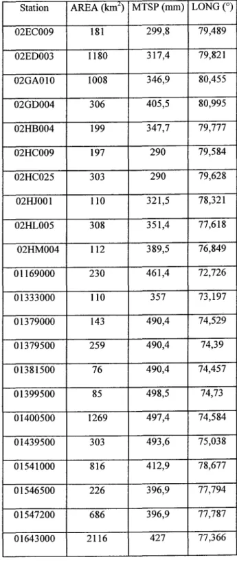
(18)

The non-stationary regional QdF model was tested on a data set of 22 gauging stations situated in eastem North America. For Ontario (Canada) gauged sites, hydrometric data were obtained from the Water Survey of Canada (Environment Canada, 2004). Data from the US sites were obtained from U.S. Geological Survey (2005). Figure 1 shows the location of the selected gauging stations. Catchments were characterized by drainage area (noted AREA, km2), mean total spring precipitation (noted MTSP, mm) and longitude (noted LONG, 0) (Environment Canada. 2004; Birikundavyi et al., 1997; USGS, 2005; Environment Canada, 2002; Carbon Dioxide Information Analysis Center, 2002). The drainage area was log-transformed for normality. Catchment areas range from 76 km2 (01381500, Whippany River at Morristown, NJ, USA) to 2116 km2 (01643000, Monocacy River at Jug bridge, near Frederick, MD, USA). Table 1 summarizes the characteristics of the stations used in the study.

Since QdF analysis takes into account the temporal variability of floods, maximum daily flows were used, but we also considered maximum daily flows averaged over different durations d. In this study, since we did not have access to an instantaneous streamflow

time series, the mean daily values correspond to the particular case where d = 1 day.

Daily values of flow averaged over different durations d were computed from the whole original streamflow time series using a moving average technique with a window of length d. In this study, we considered d = l, 5, 7, 9, 13, 15 days.

Because the region under study is subject to co Id winters, floods are mainly caused by snowmelt during the spring season. Therefore, we chose to focus on spring floods as they represent the dominant flood events in the study area. Since every selected gauging

station is located below 45° latitude, the end of the spring season was fixed at May 31 (Javelle et al., 2002; Javelle et al., 2003). For each gauging station, annual spring floods were then computed using data from the spring season.

From the data observed at the selected gaugmg stations, a common 30-year long observation period from 1974 to 2003 was identified and used in subsequent analyses. This observation period was chosen because the selected gauging stations show a significant decreasing trend (at the 90% confidence level) in the annual spring flood time series for this specific observation period according to the modified version of the Mann-Kendall test (Yue and Pilon, 2003). Figure 2 shows an exarnple of the annual spring flood time series from the gauging station 02HJOO 1. It indicates a visible decreasing trend in the time series.

5.2

Methodology

The first step of the regionalization procedure is the identification of hydrological neighborhoods by the CCA method. This approach considers each catchrnent as having its own hydrological neighborhood. In order to identify the hydrological neighborhood for each gauging station selected for this study, ajackknife procedure was used: each gauging station is in turn considered as an ungauged site and removed from the database. Then, a homogeneous region for the target-site is identified by a given method (CCA method in this study) arnong aIl the remaining gauging stations of the database. The CCA method was carried out on the basis of 2 sets of hydrological variables: stationary and non-stationary local 5-year and 100-year flood quantiles (denoted S_CCA and NS_CCA respectively). The physiographical and meteorological variables used were the drainage area (AREA) , mean total spring precipitation (MTSP) and longitude (LONG). Those variables were chosen because they were the most closely correlated with the local quantiles. The average neighborhood size was 8 and 7 catchrnents for the stationary and non-stationary cases respectively.

Stationary and non-stationary local flood frequency analyses were carried out to compute the 5-year and 100-year quantiles used in the CCA method. For the stationary case,

several statistical distributions were fitted and the best distribution for each gauging station was selected according to the Bayesian information criteria (BIC):

BIC

=

-210g(L) + 2k 10g(N) (19)

where L is the likelihood, k, the number of parameters and N, the sample size. The BIC was chosen because its model order selection criterion is based on parsimony (Box et al., 1994).

For the non-stationary case, the non-stationary OEV distribution was fitted. As suggested by El Adlouni et al. (2005) and Martins and Stedinger (2000), the generalized maximum

.

likelihood (OML) estimation method was used for parameter estimation and a Beta distribution was used as prior distribution for the shape parameter. Moreover, a homoscedastic model with location parameter linearly dependent on time was considered. Scale and shape parameters are assumed to be time-invariant.

For the assessment and comparison of the regionalization errors resulting from the CCA method, the results were compared to those obtained from a scenario where the set of aH catchments is treated as a single region and aH available information is used in the regional analysis. Thus, each gauging station was in tum considered as an ungauged site and the 21 remaining sites were considered as the homogeneous region. In the remainder of the present paper, this method will be abbreviated as the "ALL" method. The comparison of performances of the CCA method with the ALL method aHowed identifying the advantages of the identification of a hydrological neighborhood that is specifie to the site of interest.

The second and last step of the regionalization procedure was the regional estimation. Stationary and non-stationary regional QdF models (denoted S _ QdF and NS _ QdF respectively) were applied to annual spring floods from the 22 selected stations on the basis of the hydrological neighborhoods defined by the CCA and ALL methods. The physiographical and meteorological variables used for the identification of hydrological neighborhoods by the CCA method were also used in the regression models defined to

estimate the flood dynamics parameter (~) and the index flood (fi). Those variables were the drainage area (AREA) , mean total spring precipitation (MTSP) and longitude (LONG). In the regional Bootstrap re-sampling test used for the regional nonstationarity significance analysis, a 90% confidence level was used. Quantiles of the regional growth curve were estimated from the GEV distribution.

Four cases were considered: S_CCA + S_QdF, NS_CCA + NS_QdF, ALL + S_QdF and ALL + NS _ QdF. Two performance measures were computed to compare the local and regional quantile estimates. These measures are the relative mean bias (rMB) and the relative root mean squared error (rRMSE):

rMB=_1 t[QR,i -QL,i] 22 i=1 QL,i (20) rRMSE= _1 t[QR,i-QL,i]2 22'=1 QL,i (21)

where QR,i and QL,i corresponds to the regional and local T-year quantile estimates at

gauging station i. Since a significant trend was identified in the gauging stations from the

study are a, rMB and rRMSE were computed assuming that the "true local values" are the local quantiles estimated from the non-stationary GEV distribution.

5.3

Results

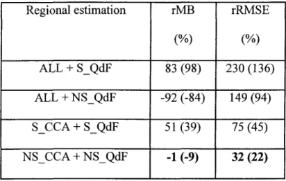
Table 2 provides the rMB and rRMSE of the QR(d = 7,T = lOO,t = 2003) quanti le for the various cases. Quantile estimates for the year 2003 were used because this year corresponds to the last year of the common observation period considered.

First of aIl, it is noticed that for the ALL method, in terms of rMB, stationary QdF modeling seems to lead to better results for the estimation of the

QR(d = 7,T = lOO,t = 2003) quantile. Indeed, the absolute rMB is larger for the ALL+QdF _NS case than for the ALL+QdF _S case. However, when the non-stationary QdF model is applied, the rRMSE is smaIler than for the stationary case. We recall that

we have: RMSE

=

.J

variance+bias2 • Therefore, although stationary QdF modeling seems

preferable in terms of bias, it leads to results having a greater variance than non-stationary QdF modeling. Figure 3 shows the results obtained for each station for the ALL+S_QdF and ALL+NS_QdF cases. It shows that for sorne stations, the two types ofQdF modeling (stationary and non-stationary) lead to important underestimations for the estimation of the QR (d

=

7, T

=

100, (

=

2003) quantile. These stations represent small basins (drainage area of approximately 100 km2). Thus, by using aIl the stations, i.e. while mixing smaIl,

average and large basins, it was not possible to obtain good estimates for these small basins. It is supposed that the index flood, estimated by regression on the basis of aIl stations, was probably underestimated what led to small values of the

QR(d

=

7,T

=

100,t

=

2003) quantile compared to the "true local values".

In addition, the results indicate that as much in terms of rMB that in terms of rRMSE, the errors obtained for the estimation of the QR (d

=

7, T

=

100, (

=

2003) quantile are smaller for the CCA method than for the ALL method. More specificaIly, for the stationary case, the CCA method does not over-estimate the QR (d

=

7, T

=

100, (

=

2003) quanti le as much as the ALL method. The same observation can be made in the non-stationary case, although, in that case, the QR(d

=

7,T

=

100,(

=

2003) quantile is underestimated. FinaIly, for the CCA method, the QR(d

=

7,T

=

100,(

=

2003) quantile estimates obtained by the non-stationary QdF are closer to the "true local values". Indeed, a rMB of -1 % is obtained for the case NS _ CCA +NS _ QdF whereas III the stationary case, the

QR (d

=

7, T

=

100, (

=

2003) quantile is over-estimated by 51 %. Figure 4 shows the results obtained for each station for the NS_CCA+NS_QdF and S_CCA+S_QdF cases. It

clearly indicates that in the NS _ CCA+NS _ QdF case, the errors obtained for the estimate ofthe QR(d

=

7,T

=

100,(

=

2003) quantile are in general smaller than the errors obtained for the S _ CCA +S _ QdF case.

Figure 5 shows a comparison of the stationary and non-stationary regional 100-year quanti le estimates for the duration of 7 days. Non-stationary local estimates and regional