WIND TURBINES TURBULENCE EFFECTS ON CABLE STRUCTURES IN THEIR VICINITY.
J.L. Lilien, R. Keutgen, N. Raimarckers University of Liège, Montefiore Electrical Institute
Sart Tilman – B.28, 4000 Liege (Belgium)
Abstract
Actual wind turbines size can be as large as 80 meters diameter (1 MW and over). Behind the wind turbines, mean wind speed is sensibly reduced (approximately 50%) and turbulence severely increased.
The spectral density power of disturbed wind can be assumed similar to classical wind but centred on the rotational speed of the motor. Due to classical speed and shape of wind turbine, corresponding
key frequency for disturbed wind is close to one Hz.
Any structure in the vicinity of wind turbine can be disturbed by the new wind spectrum created by the turbine, thus existing most of the time for wind speed up to 25 m/s.
Cable structure, f.e. overhead lines, have clearly 1 Hz in their first modal shapes. This make them very sensible to buffeting due to the disturbed wind induced by the turbine.
Due to continuous excitation, most of the year, fatigue may occur near clamping point and extra damping may be required as well as minimum distance from the wind turbine may be recommended. The anchoring tower (whose first eigenfrequency is generally close to 1 Hz for high voltage lines) will also be affected.
This paper will present some simulations of overhead lines disturbances induced by wind turbine in their vicinity. The power spectral density of wind behind the turbine will be deduced from classical spectra of Davenport, but with adaptation due to the rotation of the turbine. Effects on cable will be shown and tentative recommendations of damping as well as clearances from the turbine will be suggested.
INTRODUCTION
Basic physics gives access to the mechanical power of the rotor axis of a wind turbine [4]:
A V C P air x 3 2 1 ρ = (1)
Where A is the area swept by the rotor blades, (m2) V, the velocity of air (m/s)
Cx = power coefficient (maximum 0.593 following Betz, when downstream wind velocity is between 20 and 40 % of the upstream wind velocity)
ρair= density of ambient air (about 1.2 kg/m3) P the power in Watts
This is valid for horizontal axis turbine. These are using generally two or three blades. The minimum wind speed is around 4 m/s , the maximum one is around 25 m/s.
For example a 600 kW wind turbine with 3 blades of 21 m (swept area 1385 m2) generated in Denmark in one year 5 GWh, most of them being produced at a mean wind velocity of 8 m/s.
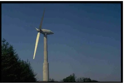
Fig. 1 Typical three blades wind turbine located in Denmark (rotor diameter 54m, 600 kW) A photo gallery available at : http://www.afm.dtu.dk/wind/turbines/gallery.html
The rotor speed is adapted to optimise power coefficient value as close as possible to its maximum to extract more energy from the wind. This is valid on the range 4 to 15 m/s, range in which power output is increasing with the cubic power of the wind speed. In the range 15 to 25 m/s it is a more or less constant power output region. There is a cut-out for larger wind speed (the large moment of inertia of the rotor – about 10000 kg.m2 – is creating large torque on the rotor during rotor speed change, which induce too large constrains for design over a certain wind speed value). The rotor speed is generally in the range of 0.5 to 2 rotations/second.
By the way the audible noise of such structure is in the range of 55 dBA at 50 m distance from the turbine.
The main purpose of this paper is to quantify the perturbation induced by such wind turbine in the vicinity of flexible structures.
The first objective will be to define the energy content of the perturbation and its frequency profile. This will be based on a logic approach based on existing data on natural wind turbulence. The wind turbine turbulence effect will be deduced from that spectrum taking into account the rotational speed of the rotor.
The second objective will be to evaluate the transient response of an overhead line span in the vicinity of the wind turbine. The buffeting response of the cable will be analysed by non-linear transient response of the cable span submitted to wind load using turbulence spectra deduced from objective one. Wind record are generated on the part of the span subject to the wake during the classical 10 minutes time period to reproduce actual situation.
The third objective is to quantify consequences on cable vibration amplitude, obviously in the range of 1 Hz and around. Fatigue approach can be analysed to see if the presence of the wind turbine can affect the life time of the cable structure in its vicinity (in a certain proximity).
Finally recommendation may be deduced for the proximity of cable structures near wind turbine not to affect their life time.
WIND MODEL [2-3]
Typical wind model
T t
( )
U z U z t( )
,( )
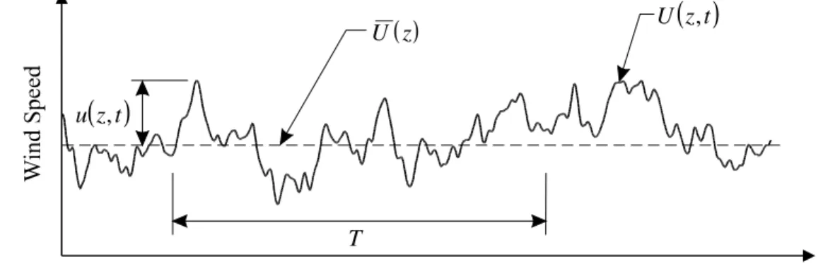
u z t,Fig. 2 Time history defining wind speed components. U(z)=mean wind speed (generally based on ten minutes sample (T=10 minutes)) at elevation z. U( tz, )=instantaneous wind speed.
Wind gusts in fact exhibit a three dimensional action, but we will obviously (having in mind a simple model for our wind turbine) limit our approach to the along wind fluctuations u
( )
z,t , parallel to the mean wind direction.Power Density Spectrum [2]: Velocity gradients within the atmospheric boundary layer initiate the formation of large eddies comparable in size to the depth of the boundary layer itself. Of an inherently unstable nature, large eddies are progressively broken down into a succession of smaller sizes. Ultimately, eddies become sufficiently small to be dissipated by the air’s viscosity. The resulting distribution of gust sizes (and duration) can be described using a power spectral density function, or spectrum, Su
( )
f , where f is the gust frequency in Hz. More specifically, a spectrumdefines the frequency content of the turbulence, with the frequency being inversely related to the gust size. The turbulence spectrum has the important property that
( )
∫
= S f f
u~2 u d (2)
In other words, the area under the spectrum is equal to the mean-square value of the wind speed fluctuations. Another common notation is using the standard deviation σ = u~2 . The longitudinal turbulence intensity is defined as :
) ( ) ( ) ( z U z z I =σ (2bis)
A more convenient form of the spectrum for both visualisation and calculation purposes is the
log-spectrum, in which the quantity f Su
( )
f is expressed as a function of the natural logarithm of thefrequency. It is easily demonstrated that
( )
∫
( ) (
)
∫
== S f f f S f f
u u d u dln
~2 (3)
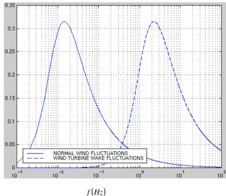
indicating that the log-spectrum describes the distribution of turbulent energy in the same way as the original spectrum. An example plot of a normalised log-spectrum ( f Su
( )
f u~2) is shown in Figure 3 for the along wind component of turbulence. Here, it is evident that the majority of the turbulent energy resides within the frequency range of approximately 0.005 Hz to 0.1 Hz, with little energy available above 1 Hz.( )
Hz f( )
2 ~ . u f S f uFig. 3 Example (10 minutes average wind speed of 10 m/s) spectrum of wind turbulence
(Davenport spectrum).(straight line) and our suggested spectrum for wind turbine turbulence spectrum. The maximum of our curve is not at 1 Hz because of the chosen ordinates. Su is maximum at 1 Hz but (f. Su ) is
max at 2.2 Hz. The chosen ordinates is made to have both curves with same maxima at around 0.32.
Although a number of expressions have been proposed for the wind spectrum, an early form proposed by Davenport (1964) [2] may be stated as
( )
(
2)
43 2 21
6
0
.
4
~
n
n
u
f
S
f
u+
=
(4)where
n
is a reduced frequency given by10
U
f
L
n
=
u (5)and Lu is a length scale (approximately equal to 1,200 m), U10 is the mean (estimated over 10
minutes) wind speed at 10 m height over the ground (in m/s), f the frequency in Hz. One characteristic of the Davenport spectrum is that it is invariant with height. Wind turbine turbulence spectrum
We have based our turbulence spectra taking into account that high energy level in power spectral density of the disturbed wind must be around 1 Hz (0.5 rotation of two blades per second means wind input is disturbed once per rotation or per second or 1 Hz).
The turbulence wake has been evaluated beyond the wind turbine and the wake is maintained over a minimum of three times blades diameter, its wake size is increasing with a slope of few degrees (3°).
Wind speed ratio is depending on wind direction but is obviously close to 0.5 (measured at 2.5 blade diameter) (see explanation based on power coefficient). At the same location normalised turbulence intensity is increased from 8% (initial wind turbulence) up to 20%.
Fig. 4 Wind speed change and turbulence effect of wind turbine [1]. The normalised turbulent intensity is defined in (2 bis) equation.
As the authors have not found appropriate data in the literature concerning the turbulence spectrum created by a wind turbine, the following approach has been considered.
1) the shape is similar as Davenport spectrum
( )
(
2)
4/3 2 21
~
n
n
u
f
S
f
uβ
α
+
=
(6)where the two numerical values have been replaced by α and β unknown values.
2) the maximum amplitude of Su(f)(which is an image of the most energetic frequency excitation) will be observed at 1 Hz, in direct correlation with the rotation of the rotor, as explained earlier. Using (5) definition, we transform (6) into :
( )
(
2)
4/3 21
~
bf
f
a
u
f
S
u+
=
(7)After derivation of (7) which must be zero at f= 1 Hz, we easily obtain :
6
.
0
=
b
(8)3) We maintain the basic condition of constant area given by the integral of the spectrum means a constant root mean square value of wind fluctuations) :
1
~
)
(
0 2=
∫
∞df
u
f
S
u (9) After some calculations, we may deduce :4
.
0
3
2
=
=
b
a
(10)A short calculation may deduce that the basic Davenport equation remain valid as formula (4), the length scale Lu (equal to 1200 m for Davenport Spectrum) has to be reduced to about 7.8 meters. In eq (5). There is obviously a relationship between that length, the mean wind speed (10m/s) and the dominant frequency at 1 Hz.. In other words, the frequency obtained by
u L
U10 must be more or less
equal to the number of blades divided by the period of the blade rotation (s).
We have no measurement results to validate such an approach, unfortunately. But the most important is to be focused now on the behaviour of flexible structure submitted to turbulences having a 1 Hz dominant energetic content.
The new spectrum is thus used to generate wind events on a 10 minutes time history to be in agreement with fig.3. This is done accordingly with some literature on the subject, not detailed here but explained in [5]. 50. 100. 150. 200. 250. 300. 350. 400. 450. 500. 550. 600. Temps. 4. 6. 8. 10. 12. 14. 16. 18.
fig.5 Generated wind at mid-span location (in front of the wind turbine wake), the mean wind is reduced to 10 m/s (50% of incoming wind) and turbulence standard deviation increased to 20%. Power spectral density as
explained in the text (formula 7 to 10). Abscissa in seconds. Ordinates in m/s. U10 = 10m/s, I = 20%.
591. 592. 593. 594. 595. 596. 597. 598. 599. 600. Temps. 4. 6. 8. 10. 12. 14. 16. 18.
Fig.6 details of the last 10 seconds of fig.5. This is the wind speed on a special location on the cable due to wind turbine wake. The frequency content is in relation with the proposed spectrum as explained in the text.
Abscissa in seconds, ordinates in m/s.
STRUCTURAL RESPONSE
Our simulation concerns a typical overhead line with a span length of 200 m (ACSR conductor, 32 mm diameter, 1.7 kg/m), supposed to be located perpendicular to the wake created by the wind turbine in its vicinity (2 to 3 times the rotor diameter).. The wind turbine rotor diameter has been fixed to 80 meters and its wake is localised as acting on the middle part of the span. The basic wind speed (before going through the wind turbine) has been fixed to 20 m/s.
It means that 80 m central part of the span is submitted to a 10 minutes average wind speed of 10 m/s plus turbulences as generated using the power spectral density shown on fig.3 and the remaining part of the span being submitted to a constant 20 m/s wind speed.
The initial sag of the conductor span is important, because it has close relationship with the eigenfrequencies of the span. A sag of 2.8 m has been chosen to have a third mode around 1 Hz (the first one being close to 0.5 Hz due to dead-end span effect).
Computations have been done using SAMCEF software (MECANO-CABLE module) which is international world-wide software using finite element model. The cable is using a non linear large displacement model. 50. 100. 150. 200. 250. 300. 350. 400. 450. 500. 550. 600. Temps. -2.4000 -2.4500 -2.5000 -2.5500 -2.6000 -2.6500 -2.7000 -2.7500 -2.8000 -2.8500 -2.9000 -2.9500 -3. -3.0500
Fig. 7 time response of the vertical displacement of the cable Disturbance caused by the sudden application of the wind (time zero) had not to be considered. Max peak-to-peak amplitude is about 15 cm.
582. 584. 586. 588. 590. 592. 594. 596. 598. 600. Temps. -2.6000 -2.6200 -2.6400 -2.6600 -2.6800 -2.7000 -2.7200 -2.7400
Fig. 8 Similar as fig.7 with a zoom on the last 8 seconds. It is quite clear that 0.5 Hz is the dominant component superimposed by other harmonics.
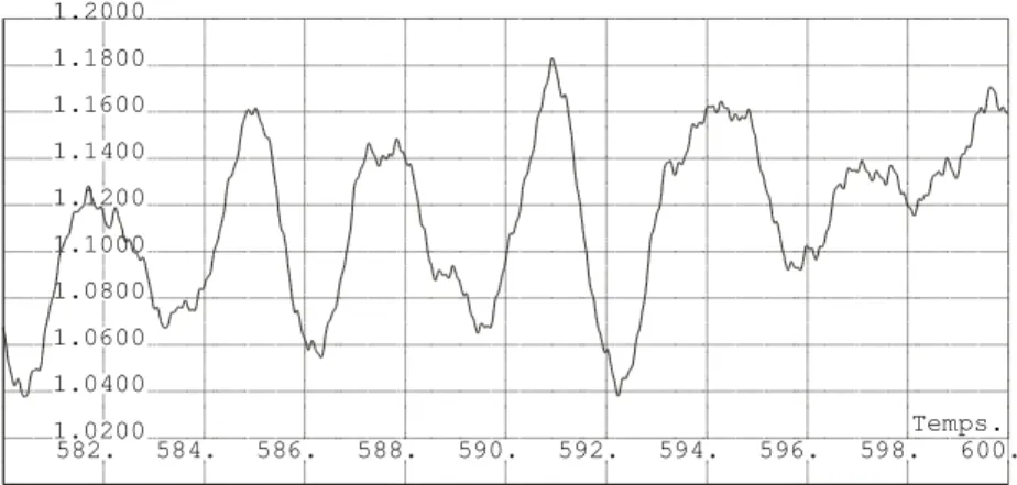
582. 584. 586. 588. 590. 592. 594. 596. 598. 600. Temps. 1.0200 1.0400 1.0600 1.0800 1.1000 1.1200 1.1400 1.1600 1.1800 1.2000
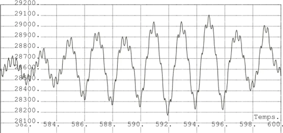
582. 584. 586. 588. 590. 592. 594. 596. 598. 600. Temps. 28100. 28200. 28300. 28400. 28500. 28600. 28700. 28800. 28900. 29000. 29100. 29200.
Fig. 10 similar as fig. 6 and 7 but for tension variation in the cable, limited to 3%. Ordinates in Newtons.
In summary, we may consider that tension variations are very limited, obviously, but that displacement amplitude can be as high as about 10 cm for 0.5 Hz component. It must be noted that , despite higher energy content in the 1 Hz zone of wind excitation, the basic first mode of the cable also received some energy (see the spectrum on fig. 3) and that one is much strongly included in the dynamic response than higher modes. A more deep analysis would be of some help to split contributions of every modes. The movement is both vertical and horizontal, which is completely different from classical Von-Karman vortex shedding vibrations.
Fatigue analysis
The fatigue phenomenon in overhead lines has been deeply studied in the literature. The number of cycles before degradation (10% of cable strands destroyed) has been defined by so called “CIGRE” curve given by the formula :[6]
z F =C.N
σ , where C = 450, z=-0.2 (minus 0.2) for less than 2.107 cycles ACSR cables. σF being the limit dynamic constrain (zero-peak) expressed in N/mm2 (or MPa) for N cycles. The bending constrain near the clamps may be obtained by the PS formula (Poffenberger-Swart)[7]
max . fy EI m dEa a π σ = (11)
Where d is the outside diameter of the cable (0.03 meter in our case), Ea is the yound modulus of the outside layer of the cable (7 1010 N/m2 in our case), m the mass per unit length of the cable (1.7 kg/m) and EI is the minimum flexural stiffness of the cable (the sum of each individual wires, that means that our 61 wires cables of 3.5 mm is giving a 67 N.m2 bending stiffness). f is the frequency (Hz) of the vibration for which we are making a fatigue analysis and ymax its amplitude in meter (zero-peak). So that max . 1100 fy a = σ (expressed in Mpa) (12)
For the 0.5 Hz (=f) with 0.05 m half amplitude (= ymax), it gives a PS constrain of about 30 Mpa, which need about 800.000 cycles or about 450 hours (18 days). So that fretting fatigue may damage the cable after such few days of excitation, means about several month to several years of operation. (our simulation has been performed with a original wind speed of 20 m/s).
It is thus strongly recommended to avoid such situation and at least to start more studies related to the definition of the power spectral density created by wind turbine and to performe fatigue analysis in all cable structure in the vicinity of about 5 times the diameter of the wind turbines (the wake effect has also to be quantified as a function of the distance from the turbine, but wake effect are known to be
active up to minimum 10 times the size of the original obstacle from which the wake is generated (by similarities with wake induced vibration on bundle conductor inpower lines).
CONCLUSIONS
Flexible structures submitted to turbulences, having a significant energy content in the frequency domain of their first eigenfrequencies, are obviously influenced. This may force displacement causing troubles for clearances. Moreover sustained oscillations are induced by turbulences, especially in the low frequency range (related to wind turbine rotor speed). This may induce ageing of structures (tower, conductor, clamps, connections, etc…). In this paper a specific case in a dramatic situation has been considered : a span having a 1 Hz (mode three) oscillation frequency and a 0.5 Hz first eigenfrequency. Moreover the wind turbine was close to the line and its diameter was covering more than one third of the whole span.
In such conditions, we have observed these results :
- the first mode is very sensible to the wake despite its very low power spectral density in that frequency range. This has induced peak-to-peak amplitudes in the range 10-15 cm both for horizontal and vertical displacement.
- The problem is not related to tension variation which is obviously limited to a few per cent of initial value
- Fretting fatigue is clearly the point, because a limited period of operation (a few month’s to a few years) with only about 20 days of high wind speed may induce wires breaking in our hypothesis of power spectral density. It would be extremely difficult to damp such low frequency vibrations. Complementary investigations are needed to qualify and quantify the turbulence spectra created by the wind turbine.
Moreover measurement of cable and tower vibration in the range 0.3-5 Hz are strongly recommended. In the meantime we would recommend a safety distance between flexible structure (as power lines) and wind turbine larger than 10 times the diameter to limit the wake effect which is known to be active up to 10 times the diameter in other field of wake induce vibrations (subspan vibration for example). Moreover we would strongly recommend to also evaluate similar effects on bundle configuration, because subspan vibration are very sensitive to the same range of frequencies.
The simulation has been performed at 1 Hz dominant energy input, but rotational speed of the rotor and the number of blades have obviously a key influence on that basic excitation frequency.
By the way, the risk of “classical” aeolian vibrations (due to Von Karman vortex shedding) is obviously reduced to zero because turbulent wind cannot input enough synchronous excitation to allow such vibrations. Only buffeting has to be considered, from the point of view of the authors. Wake induce vibrations, as observed on bundle conductors would have also to be examined because of the turbulent wake. As the wake is much larger than conductor diameter, the probability of such kind of vibration is also negligible in such situation.
REFERENCES
[1] Dr. Haubrich et al. « Untersuchung des notwendigen Mindestabstands von Windenergieanlagen
zu Freileitungen » Wissenschaftliche Studie im Auftrag des Ministerium für Wirtshaft und Mittelsland, Technologie und Verkehr des Landes Nordrhein Westfalen., Feb. 1998..
[2] E.Simiu, H. Scanlan. Wind Effects on Structures (third edition), Wiley, New York, (1996), [3] R.D. Blevins. Flow-Induced Vibration (second edition), Krieger, Malabar (1994)
[4] M.R. Patel. Wind and Solar Power Systems, CRC, London (1999)
[5] R. Keutgen, "Galloping Phenomena. A finite Element Approach", Collection des Publications de la Faculté des Sciences Appliquées de l’Université de Liège, PhD. vol. 191 (1999)
[6] Report on Aeolian vibration. Electra N°124, pp 41-77, 1989
[7] J.C. Poffenberger, R.L. Swart. Differential displacement and dynamic conductor strain. IEEE Trans on PAS, PAS-84, 1965, pp281-289
![Fig. 4 Wind speed change and turbulence effect of wind turbine [1]. The normalised turbulent intensity is defined in (2 bis) equation](https://thumb-eu.123doks.com/thumbv2/123doknet/5453547.128726/5.918.128.794.186.431/change-turbulence-turbine-normalised-turbulent-intensity-defined-equation.webp)