Improved Bayesian Network Configurations for Probabilistic Identification of Degradation Mechanisms: Application to Chloride Ingress

(1)

HAL Id: hal-01201559

https://hal.archives-ouvertes.fr/hal-01201559

Submitted on 17 Sep 2015

HAL is a multi-disciplinary open access archive for the deposit and dissemination of sci-entific research documents, whether they are pub-lished or not. The documents may come from teaching and research institutions in France or abroad, or from public or private research centers.

L’archive ouverte pluridisciplinaire HAL, est destinée au dépôt et à la diffusion de documents scientifiques de niveau recherche, publiés ou non, émanant des établissements d’enseignement et de recherche français ou étrangers, des laboratoires publics ou privés.

Improved Bayesian Network Configurations for

Probabilistic Identification of Degradation Mechanisms:

Application to Chloride Ingress

Thanh-Binh Tran, Emilio Bastidas-Arteaga, Franck Schoefs

To cite this version:

Thanh-Binh Tran, Emilio Bastidas-Arteaga, Franck Schoefs. Improved Bayesian Network Configu-rations for Probabilistic Identification of Degradation Mechanisms: Application to Chloride Ingress. Structure and Infrastructure Engineering, Taylor & Francis (Routledge): STM, Behavioural Science and Public Health Titles, 2015, pp.15. �10.1080/15732479.2015.1086387�. �hal-01201559�

(2)

Please&cite&this&paper&as:&&

T"B$Tran,$E$Bastidas"Arteaga$and$F$Schoefs$(2015).$Improved$Bayesian$network$configurations$for$ probabilistic$identification$of$degradation$mechanisms:$application$to$chloride$ingress.$Structure$and$ Infrastructure$Engineering,$pages$1–15.$http://dx.doi.org/10.1080/15732479.2015.1086387$$$$

Improved Bayesian Network Configurations for Probabilistic

Identification of Degradation Mechanisms: Application to Chloride

Ingress

Thanh-Binh Tran

LUNAM Université, Université de Nantes-Ecole Centrale Nantes, GeM, Institute for Research in Civil and Mechanical Engineering/Sea and Littoral Research Institute, CNRS UMR 6183/FR 3473, Nantes, France.

Address: 2 rue de la Houssinière BP 99208, 44322 Nantes Cedex 3 France. Phone: +33

2 51 12 55 10. email: thanh-binh.tran@univ-nantes.fr

Emilio Bastidas-Arteaga (Corresponding author)

2 51 12 55 24. email: emilio.bastidas@univ-nantes.fr

Franck Schoefs

2 51 12 55 22. email: franck.schoefs@univ-nantes.fr

This work was supported by the ERDF funding of the European Union, Interreg program, for the DuratiNet project (2009-2012 Durable Transport Infrastructure in the Atlantic Area-Network); and the ‘Pays de la Loire’ region (France) for the SI3M project (2012-2016 Identification of Meta-Model for Maintenance Strategies).

(3)

Improved Bayesian Network Configurations for Probabilistic

Identification of Degradation Mechanisms: Application to Chloride

Ingress

Probabilistic modelling of deterioration processes is an important task to plan and quantify maintenance operations of structures. Relevant material and

environmental model parameters could be determined from inspection data; but in practice the number of measures required for uncertainty quantification is conditioned by time-consuming and expensive tests. The main objective of this paper is to propose a method based on Bayesian networks for improving the identification of uncertainties related to material and environmental parameters of deterioration models when there is limited available information. The outputs of the study are inspection configurations (in space and time) that could provide an optimal balance between accuracy and cost. The proposed methodology was applied to the identification of random variables for a chloride ingress model. It was found that there is an optimal discretisation for identifying each model parameter and that the combination of these configurations minimises identification errors. An illustration to the assessment of the probability of corrosion initiation showed that the approach is useful even if inspection data is limited.

Keywords: Reliability & Risk Analysis; Identification; Bayesian network; Deterioration; Chlorides; Corrosion

1. Introduction

Chloride-induced corrosion is frequently considered as the main cause of deterioration of various types of reinforced concrete (RC) structures (bridges, wharves, off-shore platforms, marine structures, etc.) that are located close to the seashore or in contact with de-icing salts. Corrosion in reinforcing bar will affect load carrying capacity through: reduction of reinforcement cross-section, loss of bond between steel and concrete, concrete cracking and delamination (Lounis & Amleh, 2003). These

consequences will lead to the reduction of serviceability and safety levels as well as the shortening of service life in RC structures. Most of RC structures are designed for a lifetime of 50-100 years. However, under chloride-attack, important damages are reported after 10-20 years (Kumar Mehta, 2004; Poupard, L’Hostis, Catinaud, & Petre-Lazar, 2006). For these reasons, many owners of large-scale structures proposed a routine schedule for maintenance in which structures are inspected periodically (every ∆t years) to ensure optimal levels of serviceability and safety during the structural life. In infrastructure management, maintenance costs have represented a significant portion of the corrosion management budgets. Virmani (2002) reports that the annual direct cost of corrosion for highway bridges in US was about $8.3 billion, where $4.5 billion was spent on maintenance and $3.8 billion was used to replace structurally deficient bridges over 10 years

Maintenance strategies are divided into two stages: inspection and repair; in which inspection results are necessary for the diagnosis: detecting corrosion in early stages, evaluating the extent of damage as well as implementing repair measures.

(4)

Nowadays, a large number of effective condition assessment techniques consisting of destructive and non-destructive methods has been developed to facilitate the assessment of corrosion consequences in RC structures. Among non-destructive methods, visual inspection is a technique usually used for evaluating the condition of RC structures and for providing qualitative information about the condition state (Roelfstra, Hajdin, Adey, & Brühwiler, 2004); but it is currently combined with image to provide also quantitative assessment (Ghosh, Pakrashi, & Schoefs, 2011). However, its results are highly affected by environmental conditions and human errors reducing its accuracy. Semi-destructive inspection techniques (coring), on the other hand, could provide accurate inspection results, however, they are more expensive and time-consuming. Non-destructive techniques are less expensive but require still technical developments (Torres-Luque, Bastidas-Arteaga, Schoefs, Sánchez-Silva, & Osma, 2014) and specific post-treatment methods for assessing the chloride content from multi-technique measurements

(Lecieux, Schoefs, Bonnet, Lecieux, & Lopes, 2015; Ploix, Garnier, Breysse, &

Moysan, 2011). The paper will focus on quantitative methods, semi and non-destructive ones, whose common objective it to assess the chloride content profile in depth or at least near the rebar. The outputs after such inspection campaigns are discrete chloride content measurements in depth and time; the continuous monitoring is beyond the scope of this paper. Note that the information in depth gives a significant information about the chloride concentration level inside the concrete and thus on the history and it is also useful for prediction from updating of time-variant models.

In order to obtain an accurate and reliable assessment of the extent of corrosion damage, engineers and inspectors combine information from different corrosion evaluation techniques. Data collected after inspection campaigns is often used to determine parameters for chloride ingress or corrosion propagation models. This information can be after used for lifetime assessment and optimisation of maintenance strategies. This study will focus on the corrosion initiation stage that is estimated from chloride penetration models. Under natural exposure conditions, chloride ingress involves important uncertainties related mainly to material properties and exposure conditions (Bastidas-Arteaga, Chateauneuf, Sánchez-Silva, Bressolette, & Schoefs, 2011; Bastidas-Arteaga, Schoefs, Stewart, & Wang, 2013; Deby, Carcasses, & Sellier, 2008; Lounis & Amleh, 2003; Saassouh & Lounis, 2012). These uncertainties are also affected by temporal and spatial variability of associated deterioration processes and their characterisation requires larger amount of inspection data (O’Connor & Kenshel, 2013; Peng & Stewart, 2014; T. V. Tran, Schoefs, & Bastidas-Arteaga, 2013).

Nevertheless, in real practice, the number of inspections is limited by the difficulties to implement tests that increase inspection times and costs. Therefore, it is necessary to use the available information in the best way for uncertainty quantification by using statistic and/or probabilistic methods. Within this context, the Bayesian method is a reasonable choice to deal with this problem.

The Bayesian approach has been applied to problems related to chloride ingress into RC in some previous studies (De-León-Escobedo, Delgado-Hernández, Martinez-Martinez, Rangel-Ramírez, & Arteaga-Arcos, 2013; Engelund & Sorensen, 1998; Enright & Frangopol, 1999; Keßler, Fischer, Straub, & Gehlen, 2013; Ma, Zhang, Wang, & Liu, 2013; Suo & Stewart, 2009; Wang & Liu, 2010). This approach provides a comprehensive and rational framework to update the estimations based on

incorporating new information from inspection data for service-life prediction of deteriorating RC structures (Keßler et al., 2013; Ma et al., 2013; Wang & Liu, 2010) or parameter estimations (Engelund & Sorensen, 1998; Enright & Frangopol, 1999; Suo & Stewart, 2009). The application of Bayesian methods for probabilistic modelling of

(5)

chloride-induced corrosion is becoming popular and it has also been applied to multiple events in the form of Bayesian Network (BN). Deby et al. (2008) and Deby, Carcasses, & Sellier (2012) have used BN as a probabilistic approach for the assessment of

probabilistic distribution of random variables in the chloride diffusion problem. The approach seems to be robust when allowing the possibility to update the statistical distributions with new information from experimental results. Bastidas-Arteaga, Schoefs, & Bonnet (2012) proposed a procedure to identify random parameters in chloride ingress models from experimental data. In this approach, the a priori

information about statistical parameters such as type of distribution, mean and standard deviation are assumed unknown. This assumption provided a generalised approach that could be applied for real structures. Hackl (2013) proposed a framework that combines structural analysis and BN for reliability assessment. This combination allows Bayesian updating of the model with measurements, monitoring and inspection results. Recently, Ma, Wang, Zhang, Xiang, & Liu (2014) developed a BN combining in situ load testing to predict the strength degradation of bridge structures subjected to chloride attack. Nevertheless, the abovementioned studies have not optimised the utilisation of inspection data, especially when the information is limited.

The main objective of the present paper is to propose a methodology for defining appropriate BN configurations for parameter identification. Data from

numerical simulations, representing different measurement sets, will be used to propose an appropriate configuration for the identification of each model parameter. A brief description of the BN and its application for chloride ingress are presented in section 2. Section 3 introduces the problem definition and the BN implementation. Section 4 analyses the influences of different BN configurations on the identification of parameters. For each BN configuration, we also discuss about numerical issues to minimise the error in the updating process. Next, the identified parameters are

employed in Monte Carlo simulation for the assessment of the probability of corrosion initiation (section 5). An improved procedure is also suggested in this paper to optimise the evaluation when available data for updating is limited.

2. Bayesian Identification and its Application to Chloride Ingress

2.1. Introduction to Bayesian Network

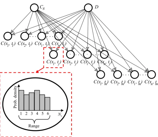
Generally, a BN is a specific type of graphical model that is represented as a Directed Acyclic Graph (DAG). Nodes in DAG are graphical representation of objects and events that exist in real world, and they are used to represent variables or deterministic states. Causal relations between nodes are represented by drawing an arc (edge)

between them. If there is a causal relationship between the variables (nodes), there will be a directional edge, leading from the cause variable to the effect variable. Each variable in the DAG has a Probability Density Function (PDF), which dimension and definition depend on the edges leading into the variables. For a set of m random variables X = [X1, X2, … , Xm], a BN represents the joint Probability Mass Function (PMF). The BN allows an efficient probabilistic modelling of complex problems by factoring the joint probability distribution into conditional probability distribution for each variable. Figure 1 describes a simple BN that consists of three nodes

corresponding to three random variables X1, X2 and X3 in which X2 and X3 are children

of the parent node X1. The children nodes have conditional probability distributions that

depend on their parent node. The parent node has a marginal probability distribution. The Bayes’ rule allows for computing the a posteriori probability p(X1| X2), given the a

(6)

priori and the conditional probabilities p(X1) and p(X2| X1): ( ) ( 2 _{( )}1) ( )1 1 2 2 | | p X X p X p X X p X = (1)

This a posteriori probability is the key of model identification from inspection data.

[Figure 1 near here]

2.2. Application to Chloride Ingress 2.2.1. Chloride Ingress and Modelling

In saturated concrete, the Fick’s diffusion equation (Tuutti, 1982) is usually used to predict the unidirectional diffusion (in x-direction):

∂Cf_c ∂t = D ∂2_C f_c ∂x2 (2)

where Cfc (kg/m3) is the concentration of chloride dissolved in pore solution, t (year) is the time and D (m/s2) is the effective chloride diffusion coefficient. Assuming that concrete is a homogeneous and isotropic material with the following initial conditions (i) the chloride concentration is zero at time t = 0 and (ii) the chloride surface

concentration is constant during the exposure time, the free chloride ion concentration

C(x,t) at depth x after time t for a semi-infinite medium is:

C x,t

( )

= Cs 1− erf x 2 D⋅t ⎛ ⎝⎜ ⎞ ⎠⎟ ⎡ ⎣ ⎢ ⎤ ⎦ ⎥ (3)

where Cs (kg/m3) is the chloride surface concentration and erf(.) is the error function. Equation (3) remains valid when RC structures are saturated and subjected to constant concentration of chlorides on the exposure surfaces. In real structures, these conditions are rarely present because concrete is a heterogeneous material and the chloride concentration in the exposed surfaces could be time-variant. Besides, this solution does not consider chloride binding capacity, concrete aging and other

environmental factors such as the influence of surrounding temperature and humidity in chloride ingress process (Bastidas-Arteaga & Stewart, 2015a, 2015b). Although this solution neglects some important physical phenomena, this model will be used herein to illustrate the proposed methodology for the identification of random variables using BN because its complexity is sufficient to account for non-linear effects in x-direction and in time and to perform sensitivity analysis: two variables are involved. The

methodology can be after extended to more realistic chloride ingress models. The computational effort for building the BN will increase for chloride ingress models involving a large number of variables.

2.2.2. Bayesian Network Modelling of Chloride Ingress

Chloride ingress could be modelled by the BN described in Figure 2 where Cs and D are the two parent nodes (random variables to identify). There are n child nodes C(xi, tj) representing the discrete chloride concentration measurement in time and space i.e. at depth xi and at inspection time tj. The number of child nodes is computed as:

x t

(7)

where nx is the total number of points in depth and nt is the total number of inspection times. Assuming that Cs and D are two independent random variables, the values of

C(xi, tj) could be easily estimated from Eq. (3). Most of parameters in chloride ingress models are defined in the continuous space. However, in order to avoid using

approximate inference algorithms which will be a disadvantage when working with continuous variables, continuous variables must be replaced by discrete random variables (Straub, 2009). Each node is defined over a specific range (upper and lower bounds) and its probability distribution is discretised into a given number of states per node, Ns. Figure 2 also illustrates the discretisation considered for each node. For this example the node C(x1,tj) was divided into Ns = 6 states over a predefined range.

In this BN, if all nodes are discrete, the probability of chloride concentration

p(C(xi, tj)) can be calculated as follows (Bastidas-Arteaga et al., 2012):

( )

(

)

(

( )

)

(

)

, , , | , , s i j i j s s D C p C x t =

∑

p C x t D C p D C with p D C

(

, _s

) ( ) ( )

=p D p C_s ₍₅₎

To estimate p(C(xi,tj)), the conditional probability p(C(xi,tj)|D,Cs) must be already known in Eq. (5). This conditional probability accounts for the dependence between the chloride content C(xi,tj) with the two model parameters (D and Cs) and it is computed based on the Conditional Probability Table (CPT) of the BN; Monte-Carlo simulations of the model (from Eq. (3)) are required for the estimation of CPT. The BN allows entering evidences and then updating the probabilities in the network. In this study, the evidences correspond to measures of chloride concentration at given points and times (chloride profiles). Then, the term p(C(xi,tj)|o) represents the probability distribution of C(xi,tj) given evidence o and a posteriori distributions of D and Cs can be computed by applying the Bayes’ theorem:

( | )

(

|

( )

i, j

)

(

( )

i, j |

)

p D o = p D C x t p C x t o with

(

( )

)

(

( )

)

( )

(

)

, | | , , i j i j i j p C x t D p D p D C x t p C x t = (6) and: ( s| )

(

s|

( )

i, j

)

(

( )

i, j |

)

p C o =p C C x t p C x t o with

(

( )

)

(

( )

)

( )

(

, |

)

| , , i j s s s i j i j p C x t C p C p C C x t p C x t = (7)

The determination of these conditional probabilities is carried out by a BN Tool Box which is built on the Matlab® Software. Note that it is assumed that the

measurements are not affected by errors. Measurement errors can be modelled by adding additional nodes to represent its PDF and its dependence on the magnitude of the measured values (Schoefs, Boéro, Clément, & Capra, 2012).

3. Problem Definition and BN Implementation

3.1. Generation of Numerical Evidences

This study aims at determining improved BN configurations for the identification of parameters of chloride ingress models. It this case, the BN will be used to update probabilistic models for the parameters to identify. The evaluation of the effectiveness of a given configuration should be based on a given criterion. Preferably, it should include a larger amount of experimental data (chloride profiles) that can be used to

(8)

estimate ‘real’ probabilistic models of model parameters and consequently to test and compare various BN configurations. However, such a database is in practice very hard to obtain because chloride profiles are computed from semi-destructive tests that are expensive and time-consuming. Therefore, in order assess the error associated to each BN configuration and to provide general recommendations that minimise the

identification errors, we consider a large number of numerical evidences (chloride profiles) generated from Monte Carlo simulations. The numerical chloride profiles are generated from theoretical probabilistic models of the random variables to identify. Table 1 presents the considered probabilistic models for Cs and D. The mean values for each parameter were taken from (Bastidas-Arteaga, Bressolette, Chateauneuf, &

Sánchez-Silva, 2009). Cs corresponds to a structure placed in an atmospheric zone, close to the seashore but without direct contact with seawater. D is a typical diffusion coefficient for ordinary Portland concrete. The COV for each parameter were reduced to 20% and 15% for Cs and D, respectively. This is due to the fact that within one type of concrete, the variation is narrowed (Duracrete, 2000; Tang & Nilsson, 1993; Vu & Stewart, 2000). The assumption that Cs and D follow lognormal distributions is also in agreement with other studies (Duracrete, 2000; Vu & Stewart, 2000).

[Table 1 near here]

The theoretical probabilistic models presented in Table 1 were used to generate 9,000 random values for Cs and D. Afterwards, each set of values of Cs and D was used to compute the 9,000 independent chloride profiles from Eq. (3). The evidences to be introduced into the BN are then computed from these chloride profiles. The same simulated values will be used for all configurations to ensure that we update the BN with the same information.

Different configurations of the BN corresponding to different inspection schemes will be analysed for selecting inspection schemes that provide the best identification of parameters. Each configuration will be evaluated in terms of the error of the identified parameter Zidentified with respect to the theoretical value Ztheory as:

( ) | identified theory|100% theory Z Z Error Z Z − = ₍₈₎

where Z represents the mean or the standard deviation of the parameter to identify – e.g. mean or standard deviation of Cs and D, Zidentified is determined from the a posteriori histograms of parent nodes (Cs and D), and Ztheory is the value of the mean or standard deviation used to generate numerical evidences (Table 1).

In practice it is unrealistic (almost impossible) to collect 9,000 chloride profiles. However, this larger database is necessary for obtaining a convergence on the error assessment. Error assessment results are after used for studying how the configuration of the BN can be improved for identification processes. The final part of the paper (section 5.2.3) will consider the improved BN configurations to study the case in which the information (number of profiles) is limited.

3.2. BN Definition and Identification Procedure

We aim at identifying the parameters Cs and D by using chloride profiles as evidences. Section 4 details the configuration of BNs considered in this study that are basically based on the general case described by Figure 2. Table 2 describes the discretisation of each node as well as the considered a priori distributions. As detailed in Figure 2, each

(9)

node is divided into Ns states over a given range. Ns will vary to determine a value that diminishes identification errors. The range (upper and lower bounds) for each parameter should in theory contain all the possible values of each parameter. These ranges can be defined on the basis of existing databases, similar study cases, or expert knowledge. Here, the ranges for Cs and D were defined enough large to contain values

representative of the variability of environmental exposure and material properties when the a priori information about these parameters is very poor. The theoretical

distributions presented in Table 2 can be used in this case to estimate upper and lower bounds for a given confidence interval. The adopted values cover a confidence interval larger than 99% by ensuring that the parameters to identify belong to this wide a priori range. A priori characteristics (type of distribution, mean, standard deviation, etc.) are commonly considered to define the configuration of the parent nodes Cs and D. To avoid hypothesis about a priori information, we suppose that Cs and D follow uniform distributions defined over given upper and lower bounds. However, if more rich a priori information is available, the consideration of this information will decrease the

identification errors. The assumption of uniform distribution for unknown parameter could avoid making any assumption about the distribution shape (Bastidas-Arteaga et al., 2012; Cao & Wang, 2014; Robinson & Hartemink, 2010). A priori distributions of parent nodes Cs and D are used to generate a sufficient random number of chloride concentrations at depth x and time t by using Eq. (3) for each child node. This a priori data is used to compute the CPT for each child node in the BN.

Data from numerical simulations will be introduced to the BN as evidences (section 3.1). The probability that C(xi,tj) belongs to a given state for different depths is then computed for the identification of the term p(C(xi,tj)|o). These probabilities are then added to the BN as soft evidences for inference. We considered an exact inference algorithm for static BN. In this process, the BN will calculate the a posteriori

distributions: p(Cs|o) and p(D|o) by using equations (6) and (7). The a posteriori distributions are after used to identify the parameter Zidentified and therefore to evaluate the error of the configuration by using Eq. (8).

The BN configurations were implemented in the Bayesian Network Toolbox (BNT) that is an open-source Matlab package for directed graphical models. This can be seen as a robust characteristic of BNT as compared with other tools because users can add, modify or make complements of functions in order to fit with the different using purposes. BNT supports many types of conditional probability distributions (nodes), many inference algorithms (exact and approximate) for both static BNs and dynamic BNs parameters and structure learning (Murphy, 2001).

4. Strategies for Improvement of BN Configurations for Parameter Identification

This section investigates the influence of the BN configuration on the identification error with respect to the theoretical parameters. We cover the following configurations:

(1) only one child node corresponding to one inspection point in depth and one inspection time (section 4.1),

(2) various child nodes corresponding to several inspection points in depth and one inspection time (section 4.2),

(3) many child nodes corresponding to several inspection points in depth and varying the inspection time (section 4.3), and

(10)

(4) various child nodes corresponding to several inspection points in depth and the combination of various inspection times (section 4.4).

Each section includes a discussion about numerical aspects that can be considered to minimise identification errors and/or decrease computational effort.

4.1. Identification Using One Inspection Point in Depth 4.1.1. Problem Statement

In this part, the estimation of the chloride surface concentration (Cs) and chloride diffusion coefficient (D) will be analysed from evidences obtained at one depth point (Figure 3). This study case could be also applied to the identification from data coming from other inspection techniques that focus on one-point measurements: resistivity based probe (Wenner probe) or resistivity basic sensors with only two points of

injection (Du Plooy, Palma Lopes, Villain, & Derobert, 2013). The BN now consists of three nodes (Figure 3): two parent nodes are Cs and D, and one child node C(xi, tj) representing the chloride concentration at depth xi. The inspection time is tins = t1 =10 years (which is compatible with actual practices) and the total inspection depth is 12cm. Consequently, we have 13 different BNs corresponding to 13 points in depth varying from 0cm to 12cm.

4.1.2. Numerical Issue: Discretisation of Child Nodes

As previously mentioned in section 3.2, continuous variables need to be discretised into several states. The number of states per node could be adjusted to obtain a balance between accuracy of results and computational time. When an accurate result is

expected, a high number of states is often chosen. Figure 4 describes the estimations of the error of the mean value of Cs with different discretisations and inspection positions in depth. It is clear that fluctuations are less important when each node C(xi,t1) in the BN is divided into Ns = 200 states. This means that a high number of states could reduce the fluctuations of the values identified by the BN. Consequently, we will use a

discretisation of Ns = 200 states per node C(xi,t1) for all BNs in this subsection.

4.1.3. Influence of Measure Depth on the Identification Error

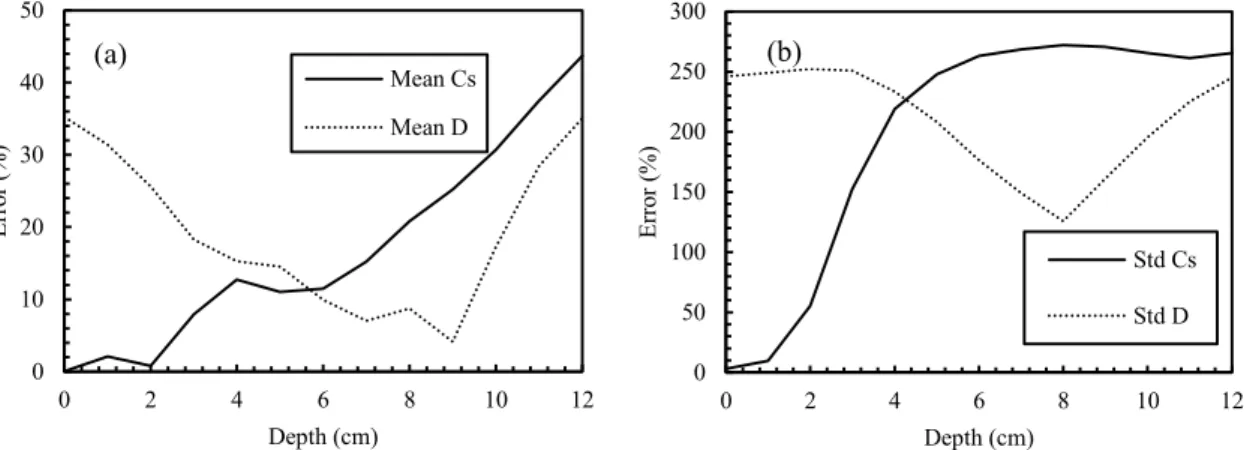
Figure 5 shows the errors in the identification of the mean and standard deviation of Cs and D. For Cs, the evolution of the error of both mean and standard deviation increase with the depth. These estimations are related to the evolution of the chloride profiles in depth. Figure 6 presents the mean chloride profile and 5% and 95% percentiles

estimated by Monte Carlo simulations from the theoretical values given in Table 1 at tins = 10 years. It is noted that chloride content is lower when depth increases. This means that, data from chloride profiles near to the surface provides more useful information for the identification of Cs, whereas less information in the deeper parts increases the error. When the chloride content is close to zero, these errors increase and they can even reach 40% for the mean. On the contrary, with the evidences near to the surface (x ≈ 0), we can obtain the best estimation for the mean and standard deviation of Cs, with errors of 1% and 3%, respectively. This is due to the fact that in eq. (3), when we set x ≈ 0,

(11)

C(xi,tj) ≈ Cs. Consequently, the chloride concentration at the surface is most valuable in the identification of Cs.

[Figure 5 near here] [Figure 6 near here]

It is also observed in Figure 5a that the error in the identification of D decreases until a depth x < 9 cm and it increases after this point. This behaviour corresponds to the fact that chloride content at deeper parts is more useful for predicting the diffusion coefficient. However, the error increases at deeper points where the chloride contents are close to zero for tins =10 years (x > 9 cm). The errors in the identification of the standard deviation of D follow a similar trend, however their values are very far from the theoretical values with important errors (more than 200%). Therefore, it can be concluded that it is very difficult to perform a good identification of D using evidences obtained from only one point in depth.

4.2. Identification Using Full Inspection Depth 4.2.1. Problem Statement

In this section, we keep the same inspection time (tins =10 years); but the BN

configuration will use data from a total inspection depth Li. The total inspection depth (Li = 12cm) is divided into several inspection points of the same discretisation size Δx. The total inspection depth is selected to cover all the potential chloride presence (see Figure 6). Figure 7 illustrates the discretisation of the total inspection length on elements of size Δx. In the experimental procedure to determine chloride profiles concrete cores are grinded over predefined discretisation sizes (equivalent to the parameter Δx) at various depths. Afterwards, an average chloride content is determined for the powder extracted at each depth. This average concentration is frequently

represented at the middle of each interval. The discretisation size Δx should not be smaller than 0.3 cm due to the accuracy of the semi-destructive equipment for determining chloride profiles. The BNs will now have a number of child nodes

depending on the total inspection depth (Li) and the adopted discretisation size (Δx). For example, if Li= 12 cm and ∆x = 2cm, the BN configuration consists of 2 parent nodes and 7 child nodes as described in Figure 7. Table 3 presents the 5 cases considered in this section where Δx varies between 0.3 cm and 3 cm.

[Table 3 near here] [Figure 7 near here]

4.2.2. Influence of the Discretisation Size ∆x on the Identification Error

Figure 8 presents the error in the identification using full inspection depth and the same ranges (boundaries) for the child nodes. These results were obtained by discretising the child nodes into 15 states. For all Δx values (BN configurations), it is noted that there is no remarkable change in the identification of the mean of Cs (Figure 8a) because the errors in 5 surveyed cases are close to 5%. Meanwhile, it seems that increasing the number inspection points might produce more errors for the standard deviation of Cs (Figure 8b). Interestingly, the gap between identified values and theoretical values for D are reduced significantly when the size of the discretisation size ∆x is smaller. The errors in the estimation of the mean of D are less than 5% when the ∆x is smaller than 0.5 cm. The standard deviation of D also reveals a better evolution when the error decreases from more than 200% with Δx=3 cm to about 20% with Δx=0.3 cm. This

(12)

behaviour is expected because when the inspection depth is divided into small ∆x, we could obtain more rich spatial information describing the level of chloride ingress that is more useful for characterising the diffusion coefficient. Hence, we can conclude that data from full inspection depth is more valuable in the identification of D.

4.2.3. Numerical Issue: Ranges for Discretising Child Nodes

As discussed in section 4.1.2, when the nodes are discretised by considering a small number of states, the errors in the estimation of chloride diffusion coefficient increase significantly. In such a case, the information used to update the BN becomes poor, particularly for deeper points where chloride content is low. For example, Figure 9a shows the evidence at depth x = 6 cm, tins = 10 years and a discretisation within Ns = 15 states. It is noted that in such a case that all the information coming from the evidences is concentrated in one state, and then, this evidence cannot provide good information for updating the BN. Increasing the number of states could solve this problem. Figure 9b indicates that Ns = 200 states are more convenient to represent the variability of the chloride concentration at this depth. Nevertheless, this solution increases the size of the CPTs and, therefore, the computational time.

In this section, we propose a procedure to improve the discretisation of child nodes. The number of states in the discretisation remains constant but we use different ranges (upper and lower boundaries) for the discretisation of all child nodes C(xi,tj). Figure 10a shows the boundaries for each node which represent for chloride content at depth x for tins = 10 yr. From a priori information of Cs and D (Table 2), Monte Carlo simulation were employed to generate a sufficient number of chloride concentration at depth x and time t from Eq. (3). From these simulations, it is possible to determine maximum and minimum values of chloride content at depth x and time t which are used as the boundaries of each child node. By considering these boundaries, we take

advantage of the information of deeper points in the updating process. Figure 10b shows the evidence at depth x = 6 cm with Ns =15 states. It is clear that the evidence at depth x

= 6 cm could provide now more valuable information for updating the BN in this case.

4.2.4. Analysis of Results for Improved Discretisation of Child Nodes

Figure 11 compares the error in the identification of the mean and standard deviation of

D before and after improvement (rebuild case) of the discretisation of child nodes. It is

clear that the consideration of large number of states and/or different ranges per node reduces drastically the errors even when the total inspection depth was divided into large Δx (Δx ∈ [2 cm, 3 cm]). This proposed approach could be very useful in practice when the number of measured points is limited or when the level of chloride content inside concrete is low.

Moreover, it is worth noticing that there are optimal discretisation sizes Δxopt: for the standard deviation (Figure 11b): Δxopt 2 cm (for Ns = 200 states) and Δxopt 1 cm (for Ns = 15 states rebuild). This means that the common idea that increasing the

number of inspection points over the total inspection depth is better is not always true for Bayesian updating. In fact, by doing so, the large error obtained by considering

(13)

some inspection depths can affect the updating: that is the case for depths with low chloride content (around x=10cm). Moreover, the difference between chloride content in adjacent inspection points is too small when the discretisation size is smaller (∆x=0.3 cm for instance). Therefore, the probability densities of the evidences used for updating the BN are very similar for two neighbouring inspection points. Figure 12a illustrates this point by showing the almost identical probabilities at x=0 cm and x=0.3 cm. This increases the errors in estimating the mean and standard deviation when using close points. In contrast, when ∆x increases (∆x = 2cm), the probability densities of the

evidences differ by reducing the identification errors (Figure 12b). That is why, even for the mean value (Figure 11a), the protocol with Δx = 3 cm is better. On the opposite, when ∆x is larger than the optimal value, the errors for both mean and standard deviation increase because the information becomes poor for describing the chloride ingress process.

4.3. Using Evidences From Different Inspection Times 4.3.1. Problem Statement

In this section, evidences obtained from various inspection times and depths will be introduced in the BN for the identification process. According to previous section, different ranges were used for each child node in the BN with a sufficient number of states per node (Ns> 15 states) to minimise the fluctuation effects/errors in the results. This analysis considers then that Ns=15 states. Since the BN configuration considers evidences coming from several inspection depths, the results of the following

subsections will be illustrated in terms of the discretisation size (Δx) in order to study the effects of considering more or less information in depth. For example, for a total inspection depth of 12 cm, the smallest value of Δx (Δx = 0.3 cm) implies that there are

nx=41 inspection points in depth. On the opposite case Δx = 12 cm considers that there are nx=2 inspection points in depth located at x=0 and x=12cm.

4.3.2. Influence of the Inspection Time on the Identification Error

Figure 13 shows the identification error for D by considering evidences taken and different inspection times tins for various discretisation sizes Δx. It can be seen that the inspection time tins influences the estimation of both the mean and standard deviation of

D. The identification is improved when tins increases until arriving at an optimal inspection value tins,opt that varies between 40 and 50 years for the identification of the mean and standard deviation. This phenomenon can be explained by the fact that when

tins ≈ 45 years the chloride concentration in the total inspection length is sufficient for describing the chloride ingress process – i.e. there is sufficient chloride content at each point in the space to improve the identification. When tins > 50 years, the chloride content at x = 12 cm is larger than zero and therefore the identification errors increase because the inspection length is not large enough to describe the problem.

It is also worth noticing to complete the analysis at the end of previous section, that there is an optimal value of Δx for each inspection time that minimises the error. The optimum value decreases when tins increases. This is related to the fact that for larger tins the chloride content inside the total inspection depth is larger. Consequently, it is necessary to add more information to improve the representation of the chloride

(14)

profile. It is also noted that the error is larger for smaller values of Δx in comparison with the Δxopt. There is no remarkable change in the estimation the mean value of D when ∆x vary from 0.3 cm to the optimal value. However, the variation is more

important for the identification of the standard deviation of D. This is mainly related to the discretisation effect described in the previous section.

For Cs, the results presented in Figure 14 reveal that it is better to use the evidences at early inspection times to obtain a better estimation of Cs. At the beginning of the exposure (e.g. tins = 1year), the chloride concentration at x ≈ 0 cm is close to Cs and it decreases drastically until zero for the neighbouring points. In such a case, the larger differences between neighbouring points (chloride concentration gradient) reduce the identification errors as indicated in Figure 12. However, when inspection times increase chlorides penetrate into concrete and the chloride concentration gradient decreases for neighbouring points by introducing inaccuracies in the assessment. The results also show that the consideration of fewer points in depth (larger Δx) diminishes significantly the errors in the assessment of the standard deviation as previously discussed in section 4.2.2.

4.4. Combining Simultaneously Evidences from Different Inspection Times 4.4.1. Problem Statement

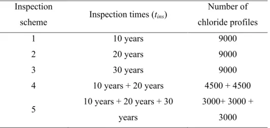
Inspection campaigns on RC structures can be carried out at different times. In this section, the BN will be used to evaluate the efficiency of combining simultaneously evidences obtained after different inspection times. For comparative purposes, we consider the same number of chloride profiles (9,000 chloride profiles) for different schemes of inspection, thus the same quantity of information for all configurations (Table 4). Thus, the evidences from each scheme may come from one inspection time or from the combination of several inspection times.

4.4.2. Identification Errors for Various Inspection Schemes

Figure 15 depicts the identification error for Cswith evidences from different schemes of inspection. As concluded in section 4.3, since the deterioration model considers that the chloride surface concentration does not depend on time, it will be better to use the evidences obtained at early inspection times. Indeed, the identification of Cs from inspection data at 10 years will be more accurate than those at 20 years or 30 years. The results in Figure 15 have pointed out that combining data from different tins could not improve the identification. For example, in the inspection scheme 4 (10+20 years), the identification errors are larger than inspection scheme 1 which uses data from tins=10 years. This is because, for the inspection scheme 4, the 4,500 chloride profiles obtained at 20 years induce errors in the identification process.

Figure 16 presents the identification errors for D with evidences for different schemes of inspection. As previously mentioned in section 4.3, evidences at tins = 30 years provide smaller identification errors than those at 10 years or 20 years. Results in Figure 16 show that from inspection scheme 3 with 9,000 chloride profiles at tins = 30 years, the estimation of D is more close to the theoretical values than others inspection schemes that use data from early inspection times or combine the evidences from

(15)

different tins. It can be also concluded that there are optimal inspection years for minimising the errors for the identification of each parameter. In this case, the

consideration of several inspection times introduced errors in the identification process. However, inspection schemes that consider several inspection times could be more appropriated to identify time-dependent parameters. For example, information of several inspection times could be useful in the identification of an ageing factor for the chloride diffusion coefficient that is considered for other models (Tran, Bastidas-Arteaga, Bonnet, & Schoefs, 2015). Although this point is important for chloride ingress modelling, the consideration of other models is beyond the scope of this paper.

4.5. Summary

Parameter identification using BN is a complex problem that requires an improved configuration to reduce identification errors. Due to physical and model characteristics, it was found that there is a best BN configuration for the identification of each

parameter. For Cs, it was the BN configuration with one child node close to the concrete surface. For D, it is necessary to use the information from total inspection length to provide a better characterisation of the kinetics of the chloride ingress process. For a certain inspection depth, an optimal inspection time exists and could describe

adequately the chloride ingress process and minimise the errors in the identification of

D. Especially, there is an optimal discretisation size for each inspection time. This

improved configuration could be considered for recommending inspection strategies. The results also revealed that it is better to use the information at early inspection times for estimating the parameter Cs; for D, the data at later and specific inspection times is more useful.

5. Assessment of the Probability of Corrosion Initiation

5.1. Probability of Corrosion Initiation

This section examines the influence of the data identified from BN on the evaluation of the probability of corrosion initiation. In fact, previous sections have shown that there are different improved configurations for the identification of Cs and D: a multi-criteria analysis will not be efficient because the sensitivity of the response to these variables vary with time (Bastidas-Arteaga et al., 2011). Thus the quantity of interest ‘probability of corrosion initiation’, useful for decision makers, is considered now. The time to corrosion initiation, tini, is defined as the time at which the chloride concentration at the steel reinforcement surface reaches a threshold value, Cth. This threshold concentration represents the chloride concentration for which the rust passive layer of steel is

destroyed and the corrosion reaction begins. Cth depends on many parameters (Bastidas-Arteaga & Schoefs, 2012): type and content of cement, exposure conditions, time and type of exposure, distance to the sea, oxygen availability at the bar depth, type of steel, electrical potential of the bar surface, presence of air voids, definition of corrosion initiation, methods and techniques for measuring Cth, etc. Then, the determination of an appropriate Cth becomes a major challenge for the owner/operator and it will be

therefore assumed herein that Cth is a random variable. The time to corrosion initiation is calculated by evaluating the time-dependent variation of the chloride concentration at the reinforcing steel depth that is computed from Eq. (3). The cumulative distribution

(16)

function of the time to corrosion initiation, F_t_ini

( )

t , is defined as:

( ) (

)

( )

ini ini t ini t t F t p t t f x dx ≤ = ≤ =

∫

₍₉₎

where f(x) is the joint PDF of the vector of random variables X. The limit state function that defines corrosion initiation can be written as:

( )

, _th

( )

_tc

( )

,

g Xt =C X −C Xt (10)

where Ctc(X, t) is the total concentration of chlorides at the concrete cover depth, ct, at time t. The probability of corrosion initiation, pini, is obtained by integrating the joint probability function over the failure domain – i.e., Eq. (10). pini is estimated herein by using Monte Carlo simulations.

5.2. Numerical Example 5.2.1. Problem Description

Lets consider a RC component placed in a chloride-contaminated environment. The parameters describing the exposure (Cs) and material properties (D) are described in Table 1. The probability of corrosion initiation is computed by considering that the threshold of chloride concentration for initiation of corrosion follows an uniform distribution with following parameters:

(

3 3

)

0.9 / ; 0.2 / th

C =U µ= kg m σ = kg m (Vu & Stewart, 2000) and a concrete cover depth of 6 cm.

We will consider various inspection schemes considering one point or various points in depth for a single inspection time tins = 10 years. The study considers different ranges for the discretisation of each child node. We will also study the case in which the number of chloride profiles is limited and we will propose a strategy to improve the assessment in such a case.

The histograms obtained after updating the BN for each parameter will be used directly in Monte Carlo simulations to estimate the probability of corrosion initiation to avoid any assumption about analytical distribution laws.

5.2.2. Assessment of pini for Larger Inspection Data

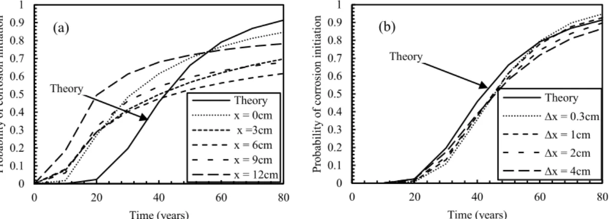
Figure 17a presents the probability of corrosion initiation with data obtained from a single point inspection depth (section 4.1). These results were obtained by identifying each parameter from 9,000 numerical chloride profiles. The results indicate that, data identified from one depth point does not provide an acceptable prediction of the

probability of corrosion initiation in comparison with the theoretical assessment (section 4.1). Although the errors in the identification of Cs are low for this inspection strategy, the errors of the identification of D introduce larger differences in the assessment of pini. However, from Figure 17b, it is noted that the prediction of the probability of corrosion initiation is more close to the theoretical values when the parameters are identified from several inspection points (section 4.2). In this case, the consideration of more inspection points reduces identification errors by improving the assessment of pini. The error depends on the ‘time of interest’ or ‘target probability of corrosion initiation’. This latter is more suitable because it is in link with actual recommendations schemes. By considering a target probability of corrosion lower than 0.5, larger values of Δx provide

(17)

a better assessment. If a higher probability of corrosion is acceptable (between 0.6 and 0.9), the opposite trend is observed.

5.2.3. Assessment of pini for Limited Inspection Data

The results presented above considered a large number of simulations for the generation of numerical evidences. However, in real practice, the number of profiles collected after an inspection campaign is very limited. Figure 18a presents the probability of corrosion initiation estimated with limited data obtained by considering the full inspection length. In this case, the numerical evidences were generated from 15 profiles of chloride content obtained from Monte Carlo simulations. It is noted that the assessment of the probability of corrosion initiation is far from the theoretical values. Consequently, it is necessary to improve the use of the information utilised for updating the BN. To improve the identification, it is proposed to combine results of BN configurations with one and several inspection points (Figure 19). We use therefore the results of the identification of Cs obtained with one depth point configuration (Step 1) as a priori data for the estimation of D by considering the full depth configuration (Step 2).

[Figure 18 near here] [Figure 19 near here]

The assessments of probability of corrosion initiation that compare these two cases (before and after improvement) are shown in Figure 18. It is clear that this

strategy improves the identification when data is limited. It could be concluded that this approach would be very useful for limited data. The assessment could be improved if we consider data of other inspection times as mentioned in section 4.3.

6. Conclusions

Chloride ingress is one of the main causes inducing corrosion of RC structures. The identification of parameters in chloride ingress modelling is crucial in predicting chloride ingress into concrete that will help to reduce maintenance costs of structures exposed to chloride-contaminated environments. Inspection data used for the

identification is very limited due to time-consuming and expensive tests. Therefore, it is necessary to use these data in an optimal scheme. Within this framework, the BN could provide a possibility to identify model parameters with different information. In this study, results based on numerical evidences revealed that there are optimal

configurations of BN for the identification of each parameter (Cs or D). For Cs, an early inspection with one point close to the surface could provide a good identification. For

D, the identification should use the evidences from full inspection depth. At a specific

inspection time, there is an optimal discretisation size that could provide the best estimation for D. These configurations could be combined to improve the identification of the model parameters. An application to the assessment of the probability of

corrosion initiation showed that the approach is useful even if information is limited. When the number of chloride profiles is limited it is required to improve: (i) the BN configuration, and (ii) the updating strategy (a two-step procedure is proposed).

This study focused on identification of model parameters for a simple analytical chloride ingress model. Tran et al., 2015 found that the main findings of this study for improving the identification of Cs and D are also valid for more complex models that account for instance for the time-dependency of D as the proposed in (Nilsson & Carcasses, 2004). However, the identification of parameters for more complex models

(18)

requires developing other BN configurations, larger computational efforts and additional inspection data. In addition, further work in this area will focus on:

• the use of real data (real chloride profiles and/or study cases),

• the consideration of other deterioration models numerical or analytical that account for more realistic conditions: unsaturated zones, binding, time-dependency of model parameters, etc,

• the consideration of measurement errors and model uncertainty,

• the extension of the identification of random variables to the identification of random fields parameters, and

• the consideration of costs for recommending inspection procedures (inspection times, number of cores, number and positions of measures in each core, etc) that provide a balance between error and cost.

7. References

Bastidas-Arteaga, E., Bressolette, P., Chateauneuf, A., & Sánchez-Silva, M. (2009). Probabilistic lifetime assessment of RC structures under coupled corrosion–fatigue deterioration processes. Structural Safety, 31(1), 84–96. doi:10.1016/j.strusafe.2008.04.001

Bastidas-Arteaga, E., Chateauneuf, A., Sánchez-Silva, M., Bressolette, P., & Schoefs, F. (2011). A comprehensive probabilistic model of chloride ingress in unsaturated concrete. Engineering Structures, 33(3), 720–730. doi:10.1016/j.engstruct.2010.11.008

Bastidas-Arteaga, E., & Schoefs, F. (2012). Stochastic improvement of inspection and maintenance of corroding reinforced concrete structures placed in unsaturated environments. Engineering Structures, 41, 50–62. doi:10.1016/j.engstruct.2012.03.011

Bastidas-Arteaga, E., Schoefs, F., & Bonnet, S. (2012). Bayesian identification of uncertainties in chloride ingress modeling into reinforced concrete structures. In

Third International Symposium on Life-Cycle Civil Engineering. Vienna, Austria.

Bastidas-Arteaga, E., Schoefs, F., Stewart, M. G., & Wang, X. (2013). Influence of global warming on durability of corroding RC structures: A probabilistic approach.

Engineering Structures, 51, 259–266. doi:10.1016/j.engstruct.2013.01.006

Bastidas-Arteaga, E., & Stewart, M. G. (2015a). Damage risks and economic assessment of climate adaptation strategies for design of new concrete structures subject to chloride-induced corrosion. Structural Safety, 52, 40–53. doi:10.1016/j.strusafe.2014.10.005

Bastidas-Arteaga, E., & Stewart, M. G. (2015b). Economic Assessment of Climate Adaptation Strategies for Existing RC Structures Subjected to Chloride-Induced Corrosion. Structure and Infrastructure Engineering, In press, 11 pages. doi:10.1080/15732479.2015.1020499

(19)

Cao, Z., & Wang, Y. (2014). Bayesian model comparison and selection of spatial correlation functions for soil parameters. Structural Safety.

doi:10.1016/j.strusafe.2013.06.003

De-León-Escobedo, D., Delgado-Hernández, D.-J., Martinez-Martinez, L.-H., Rangel-Ramírez, J.-G., & Arteaga-Arcos, J.-C. (2013). Corrosion initiation time updating by epistemic uncertainty as an alternative to schedule the first inspection time of pre-stressed concrete vehicular bridge beams. Structure and Infrastructure

Engineering, 10(8), 1–13. doi:10.1080/15732479.2013.780084

Deby, F., Carcasses, M., & Sellier, A. (2008). Toward a probabilistic design of reinforced concrete durability: application to a marine environment. Materials and

Structures, 42(10), 1379–1391. doi:10.1617/s11527-008-9457-8

Deby, F., Carcasses, M., & Sellier, A. (2012). Simplified models for the engineering of concrete formulations in a marine environment through a probabilistic method.

European Journal of Environmental and Civil Engineering, 16(3-4), 37–41.

Du Plooy, R., Palma Lopes, S., Villain, G., & Derobert, X. (2013). Development of a multi-ring resistivity cell and multi-electrode resistivity probe for investigation of cover concrete condition. NDT&E International, 54, 27–36.

Duracrete. (2000). Probabilistic calculations. DuraCrete—probabilistic performance

based durability design of concrete structures. EU—brite EuRam III. Contract BRPR-CT95-0132. Project BE95-1347/R12-13.

Engelund, S., & Sorensen, J. D. (1998). A probabilistic model for chloride-ingress and initiation of corrosion in reinforced concrete structures. Structural Safety, 20(1), 69–89.

Enright, M. P., & Frangopol, D. M. (1999). Condition prediction of deteriorating concrete bridges using Bayesian updating. Journal of Structural Engineering

ASCE, 125(10), 1118–1125.

Ghosh, B., Pakrashi, V., & Schoefs, F. (2011). High dynamic range image processing for non-destructive-testing. European Journal of Environmental and Civil

Engineering, 15(7), 1085–1096. doi:10.1080/19648189.2011.9695295

Hackl, J. (2013). Generic Framework for Stochastic Modeling of Reinforced Concrete

Deterioration Caused by Corrosion. PhD Thesis, Norwegian University of Science

and Technology.

Keßler, S., Fischer, J., Straub, D., & Gehlen, C. (2013). Updating of service - life prediction of reinforced concrete structures with potential mapping. Cement and

Concrete Composites, 47, 47–52.

Kumar Mehta, P. (2004). High-performance, high-volume fly ash concrete for sustainable development. In International Workshop on Sustainable Development

(20)

Lecieux, Y., Schoefs, F., Bonnet, S., Lecieux, T., & Lopes, S. P. (2015). Quantification and uncertainty analysis of a structural monitoring device: detection of chloride in concrete using DC electrical resistivity measurement. Nondestructive Testing and

Evaluation, 1–17. doi:10.1080/10589759.2015.1029476

Lounis, D. Z., & Amleh, L. (2003). Reliability-Based Prediction of Chloride Ingress and Reinforcement Corrosion of Aging Concrete Bridge Decks. In Proceeding of the

3rd International IABMAS Workshop on Life-Cycle Cost Analysis and Design of Civil Infrastructure Systems (pp. 139–147). Lausanne, Switzerland.

Ma, Y., Wang, L., Zhang, J., Xiang, Y., & Liu, Y. (2014). Bridge Remaining Strength Prediction Integrated with Bayesian Network and In Situ Load Testing. Journal of

Bridge Engineering ASCE, 19(10), 1–11.

doi:10.1061/(ASCE)BE.1943-5592.0000611.

Ma, Y., Zhang, J., Wang, L., & Liu, Y. (2013). Probabilistic prediction with Bayesian updating for strength degradation of RC bridge beams. Structural Safety, 44, 102– 109. doi:10.1016/j.strusafe.2013.07.006

Murphy, K. P. (2001). The Bayes Net Toolbox for Matlab.

Nilsson, L.-O., & Carcasses, M. (2004). Models for chloride ingress into concrete – A

critical analysis. Report on task 4.1, EU project “ChlorTest” G6RD-CT-2002-0085. Lund.

O’Connor, A., & Kenshel, O. (2013). Experimental Evaluation of the Scale of Fluctuation for Spatial Variability Modeling of Chloride-Induced Reinforced Concrete Corrosion. Journal Of Bridge Engineering, 18(1), 3–14.

Peng, L., & Stewart, M. G. (2014). Spatial time-dependent reliability analysis of corrosion damage to RC structures with climate change. Magazine of Concrete

Research, 66(22), 1154–1169. doi:10.1680/macr.14.00098

Ploix, M.-A., Garnier, V., Breysse, D., & Moysan, J. (2011). NDE data fusion to improve the evaluation of concrete structures. NDT & E International, 44(5), 442– 448. doi:10.1016/j.ndteint.2011.04.006

Poupard, O., L’Hostis, V., Catinaud, S., & Petre-Lazar, I. (2006). Corrosion damage diagnosis of a reinforced concrete beam after 40 years natural exposure in marine environment. Cement and Concrete Research, 36, 504–520.

Robinson, J. W., & Hartemink, A. J. (2010). Learning Non-Stationary Dynamic Bayesian Networks. The Journal of Machine Learning Research, 11, 3647–3680. Roelfstra, G., Hajdin, R., Adey, B., & Brühwiler, E. (2004). Corrosion evolution in

bridge management systems and corrosion-induced deterioration. Journal of

Bridge Engineering ASCE, 9, 268–277.

Saassouh, B., & Lounis, Z. (2012). Probabilistic modeling of chloride-induced corrosion in concrete structures using first- and second-order reliability methods.

(21)

Cement and Concrete Composites, 34(9), 1082–1093. doi:10.1016/j.cemconcomp.2012.05.001

Schoefs, F., Boéro, J., Clément, A., & Capra, B. (2012, June). The αδ method for modelling expert judgement and combination of non-destructive testing tools in risk-based inspection context: application to marine structures. Structure and

Infrastructure Engineering. doi:10.1080/15732479.2010.505374

Straub, D. (2009). Stochastic Modeling of Deterioration Processes through Dynamic Bayesian Networks. Journal of Engineering Mechanics, 135(10), 1089–1099. Suo, Q., & Stewart, M. G. (2009). Corrosion cracking prediction updating of

deteriorating RC structures using inspection information. Reliability Engineering

& System Safety, 94(8), 1340–1348. doi:10.1016/j.ress.2009.02.011

Tang, L., & Nilsson, L. O. (1993). Chloride binding capacity and binding isotherms of {OPC} pastes and mortars. Cement and Concrete Research, 23, 247–253.

Torres-Luque, M., Bastidas-Arteaga, E., Schoefs, F., Sánchez-Silva, M., & Osma, J. F. (2014). Non-destructive methods for measuring chloride ingress into concrete: State-of-the-art and future challenges. Construction and Building Materials, 68, 68–81. doi:10.1016/j.conbuildmat.2014.06.009

Tran, T. V., Schoefs, F., & Bastidas-Arteaga, E. (2013). Risk-Based-optimization of geo-positioning of sensors in case of spatial fields of deterioration / properties. In

11th International Conference on Structural Safety & Reliability. New York, USA.

Tran, T.-B., Bastidas-Arteaga, E., Bonnet, S., & Schoefs, F. (2015). Parameter identification in chloride ingress from accelerated test using bayesian network. In

12th International Conference on Applications of Statistics and Probability in Civil Engineering, ICASP12 (p. 8 pp). Vancouver, Canada.

Tuutti, K. (1982). Corrosion of steel in concrete. Swedish Cement and Concrete

Institute.

Virmani, Y. P. (2002). Corrosion costs and preventive strategies, Publication No .

FHWA-RD-01-156.

Vu, K. A. T., & Stewart, M. G. (2000). Structural reliability of concrete bridges including improved chloride-induced corrosion. Structural Safety, 22, 313–333. Wang, J., & Liu, X. (2010). Evaluation and Bayesian dynamic prediction of

deterioration of structural performance. Structure and Infrastructure Engineering,

(22)

List of Tables

Table 1: Theoretical values of parameters to identify Table 2: Discretisation of nodes and a priori distributions Table 3: Discretisation cases and number of points in depth

(23)

List of Figures

Figure 1: A Simple Bayesian Network

Figure 2: General BN configuration for modelling chloride ingress Figure 3: BN configuration using one inspection point in depth

Figure 4: Identification error of the mean value of Cs for child nodes discretised into different number of states

Figure 5: Identification error using one depth point: (a) Mean – (b) Standard deviation Figure 6: Mean chloride profile and 5% and 95% percentiles at tins=10 years

Figure 7: BN configuration with ∆x=2cm

Figure 8: Identification error using full inspection depth: (a) Mean – (b) Standard deviation

Figure 9: Evidence at x=6cm with different discretisation of child nodes: (a) 15 states – (b) 200 states

Figure 10: (a) Ranges for each child node at depth x –(b) Evidence at x=6cm with 15 states for each child node and different ranges.

Figure 11: Identification error of D for three discretisations of child nodes: (a) Mean – (b) Standard deviation

Figure 12: Effect of discretisation size ∆x on the distribution of chloride content: (a) ∆x=0.3 cm – (b) ∆x=2 cm

Figure 13: Identification error for D with evidences from different inspection times: (a) Mean - (b) standard deviation

Figure 14: Identification error for Cs with evidences from different inspection times: (a) Mean - (b) standard deviation

Figure 15: Identification error for Cs with evidences from different schemes of inspection: (a) mean - (b) standard deviation

Figure 16: Identification error for D with evidences from different schemes of inspection: (a) mean - (b) standard deviation

Figure 17: Probability of corrosion initiation with data obtained: (a) from a single point inspection depth - (b) from full inspection depth

Figure 18: Probability of corrosion initiation with limited data: (a) before improvement - (b) after improvement

(24)

Table 1: Theoretical values of parameters to identify Parameters Distribution Mean COV

Cs Lognormal 2.95 kg/m3 0.20

D Lognormal 1.33×10-12_m2_/s _0.15

Table 2: Discretisation of nodes and a priori distributions Parameters Number of states per node

(Ns) A priori distribution Range Cs (kg/m3) variablea Uniform [0.5; 8] D (m2/s) variablea Uniform [6×10-13; 3×10-12] C(xi,tj) (kg/m3) variablea b [0; 8] a _N

s varies to determine a value that diminishes the identification error

b _{Computed from a priori information of parent nodes}

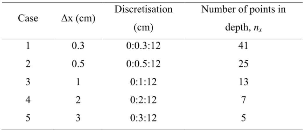
Table 3: Discretisation cases and number of points in depth Case Δx (cm) Discretisation (cm) Number of points in depth, nx 1 0.3 0:0.3:12 41 2 0.5 0:0.5:12 25 3 1 0:1:12 13 4 2 0:2:12 7 5 3 0:3:12 5

(25)

Table 4: Schemes for combining evidences for different inspection times Inspection

scheme Inspection times (tins)

Number of chloride profiles 1 10 years 9000 2 20 years 9000 3 30 years 9000 4 10 years + 20 years 4500 + 4500 5 10 years + 20 years + 30 years 3000+ 3000 + 3000

(26)

Figure 1: A Simple Bayesian Network

Figure 2: General BN configuration for modelling chloride ingress

X

₂

X

₃

X

₁ Cs D C(x , t )₁ ₁ C(x , t )₂ ₁ C(x , t )_{i 1} C(x , t )_{n 1} C(x , t )_{1 j} C(x , t )_{2 j} C(x , t )_i _j C(x , t )_{n j} C(x , t )_{1 m} C(x , t )_{2 m} C(x , t )_{i m} C(x , t )_{n m} . . . . . . . . . . . . . . . . . . 1 2 3 4 5 6 P rob. de ns it y Ns Range