HAL Id: hal-01177902
https://hal.inria.fr/hal-01177902
Submitted on 17 Jul 2015
HAL is a multi-disciplinary open access
archive for the deposit and dissemination of
sci-entific research documents, whether they are
pub-lished or not. The documents may come from
teaching and research institutions in France or
abroad, or from public or private research centers.
L’archive ouverte pluridisciplinaire HAL, est
destinée au dépôt et à la diffusion de documents
scientifiques de niveau recherche, publiés ou non,
émanant des établissements d’enseignement et de
recherche français ou étrangers, des laboratoires
publics ou privés.
Tracing Flow Information for Tighter WCET
Estimation: Application to Vectorization
Hanbing Li, Isabelle Puaut, Erven Rohou
To cite this version:
Hanbing Li, Isabelle Puaut, Erven Rohou. Tracing Flow Information for Tighter WCET
Estima-tion: Application to Vectorization. 21st IEEE International Conference on Embedded and Real-Time
Computing Systems and Applications, Aug 2015, Hong-Kong, China. pp.10. �hal-01177902�
Tracing Flow Information for Tighter WCET
Estimation: Application to Vectorization
Hanbing Li
Inria/IRISA [email protected]Isabelle Puaut
University of Rennes 1/IRISAErven Rohou
Inria/IRISA [email protected]Abstract—Real-time systems have become ubiquitous, and many play an important role in our everyday life. For hard real-time systems, computing correct results is not the only requirement. In addition, these results must be produced within pre-determined deadlines. Designers must compute the worst-case execution times (WCET) of the tasks composing the system, and guarantee that they meet the required timing constraints. Standard static WCET estimation techniques establish a WCET bound from an analysis of the machine code, taking into account additional flow information provided at source code level, either by the programmer or from static code analysis. Precise flow information helps produce tighter WCET bounds, hence limiting over-provisioning the system. However, flow information is diffi-cult to maintain consistent through the dozens of optimizations applied by a compiler, and the majority of real-time systems simply do not apply any optimization.
Vectorization is a powerful optimization that exploits data-level parallelism present in many applications, using the SIMD (single instruction multiple data) extensions of processor instruc-tion sets. Vectorizainstruc-tion is a mature optimizainstruc-tion, and it is key to the performance of many systems. Unfortunately, it strongly impacts the control flow structure of functions and loops, and makes it more difficult to trace flow information from high-level down to machine code. For this reason, as many other optimizations, it is overlooked in real-time systems.
In this paper, we propose a method to trace and maintain flow information from source code to machine code when vectorization optimization is applied. WCET estimation can benefit from this traceability. We implemented our approach in the LLVM compiler. In addition, we show through measurements on single-path programs that vectorization not only improves average-case performance but also WCETs. The WCET improvement ratio ranges from 1.18x to 1.41x depending on the target architeture on a benchmark suite designed for vectorizing compilers (TSVC).
I. INTRODUCTION
Real-time systems are increasingly present in every aspect of our lives. To be correct, these systems must deliver their results within precise deadlines. Designers of such systems must compute Worst-Case Execution Times (WCET) of the various tasks composing these systems, and guarantee that they meet the timing constraints. For critical systems, missing a deadline may have catastrophic consequences, WCET bounds must be strict upper bounds of any possible execution time [1]. To be more useful, WCET bounds should be as tight as possible, i.e. the estimated WCET should be as close as possible to the real WCET. This avoids over-provisioning processor resources, and helps keep the overall cost low.
WCET bounds must be calculated at machine code level, because the timing of processor operations can only be
ob-tained at this level. However, knowledge of flow information, that can more easily be obtained at source code level than at binary level, helps obtaining tight bounds. Flow information is for example loop bound information (the maximum number of times a loop iterates) or information on infeasible paths (paths that are structurally feasible but will never be executed whatever the input data). Flow information may be extracted automatically from source code by static analysis, but it may also be manually inserted by application developers and domain specialists.
Compilers translate the high-level source code written by programmers into machine code fit for microprocessors. During this process, modern compilers apply many optimiza-tions to deliver more performance for specific architecture and instruction sets. Because some of these optimizations significantly modify the program control flow, flow information extracted at source code level might not be correct anymore at the binary code level. If loops bounds are considered as example of flow information, considering the same loop bound at binary code level may lead to overestimated WCETs (for example when the loop is unrolled by the compiler), may not make sense (if the loop can be fully unrolled and disappears from the binary) or worse, lead to underestimated WCETs (for loop re-rolling for instance). Thus, to be safe, flow information has to be continuously updated, the transformation depending on the semantics of each actual optimization.
There have been a number of research studies on how to trace flow information within optimizing compilers for WCET estimation. Many standard optimizations are supported so far, but we are not aware of any work focusing on vectorization. This is the focus of this paper.
Vectorization has been popularized by the Intel Pentium processor for multimedia applications with the MMX fam-ily. The key idea consists in applying the same operation (arithmetic, logic, memory access) to multiple data at once (SIMD – single instruction, multiple data). They have become increasingly important in many fields, e.g. video games, 2D/3D graphics, scientific computation, and in the context of hard real-time systems, signal processing applications (sound, im-ages, video). All silicon vendors have developed their SIMD extensions: SSE and AVX on Intel/AMD processors, ARM’s NEON, PowerPC’s AltiVec... The goal of vectorization is to identify code regions that repeatedly apply given operations to consecutive data elements, and to re-arrange the computation to benefit from SIMD extensions.
In most cases, vectorization modifies the program control flow, modifying loop bounds of existing loops, adding new loops and also new if-statements. From a WCET estimation perspective, guessing from the outside what the compiler did
is far from trivial and error-prone. Relevant flow-information provided at source code level can hardly be exploited as it becomes difficult – if not impossible – to transform and attach to the correct code region. In the best case, control flow may remain identical (no new loop is introduced), but using unmodified loop bounds would be extremely pessimistic, resulting in overestimated WCET.
In this paper, we provide a method to trace flow infor-mation through vectorization, enabling complete traceability from source code level to machine code level. The flow information is transformed within the compiler in parallel with code transformation. When the compiler vectorizes the code, the flow information is traced and updated accordingly. Then, the final flow information can be conveyed to WCET analysis tools and used for the WCET calculation. This work builds upon our previous work on traceability of flow information throughout compiler optimizations [2], which so far did not consider vectorization.
We integrated our proposed method into the LLVM com-piler infrastructure. For the scope of this paper, our exper-iments in LLVM will concentrate only on loop bounds as sources of flow information.
In addition, we show through measurements on single-path programs that vectorization not only improves average-case performance but also WCETs. The WCET improvement ratio ranges from 1.18× to 1.41× depending on the target architecture on a benchmark suite designed for vectorizing compilers (TSVC).
The paper contributions are threefold:
• We propose a mechanism to trace flow information for a compiler optimization which to our best knowledge was not considered before, namely vectorization; • The traceability mechanism was integrated into the
state-of-the-art compiler LLVM;
• We show using measurements that vectorization does not only reduce average-case execution times but also reduces worst-case execution times. The experimental results we provide do not directly validate our method, but rather motivates the need to use vectorization in hard real-time systems.
Note that our objective is not to assess or improve the quality of vectorization. Instead, we consider an existing im-plementation of vectorization and we add the capability to trace flow information such that it also helps improving WCET.
The remainder of the paper is organized as follows. Sec-tion II describes the WCET calculaSec-tion method used, and gives an overview of our framework for tracing flow information. Section III presents the main contributions of our work. It first introduces vectorization technology and details how flow information is traced with our framework during vectorization, independently of the compiler framework. The implementation within the LLVM compiler infrastructure is then introduced. Experimental setup, results and their analysis are presented in Section IV. Related work is surveyed in Section V. We finally conclude with a summary of the paper contributions and plans for future work.
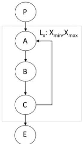
Fig. 1: Example of control flow graph (CFG)
II. BACKGROUND: WCETCALCULATION AND TRACEABILITY OF FLOW INFORMATION
This section presents the WCET calculation technique used throughout the paper (§ II-A) and gives an overview of the framework we are using for tracing flow information (§ II-B), in which vectorization was integrated.
A. WCET calculation methods
WCET calculation methods can be classified into two categories: static and measurement-based methods [1]. Static methods calculate WCETs, without any execution, based on the analysis of the set of possible control flow paths from the code structure. We use the most common static WCET calcula-tion method for WCET calculacalcula-tion: implicit path enumeracalcula-tion technique(IPET) [3]. IPET extracts control flow graphs (CFG) from binary code, and models the WCET calculation problem as an Integer Linear Programming (ILP) system by combining the flow information in the CFG and additional constraints specifying flow information that cannot be obtained directly from the control flow graph (e.g. loop bounds, infeasible paths).
An example CFG is shown in Figure 1. The nodes N , representing basic blocks, are depicted as circles in this fig-ure. The edges E are the arrows representing possible flows between basic blocks. This example can be expressed as:
CFG = {N , E} N = {P, A, B, C, E}
E = {P → A, A → B, B → C, C → A, C → E} For this CFG, the ILP system in Figure 2 can be used to calculate the WCET. In this system, for basic block i, fi
represents its execution count and Ti represents its
worst-case execution time. In order to calculate the WCET, the objective function should be maximized. Flows in the CFG are constrained by structural constraints extracted from the CFG in which fij represents the execution count of the edges from
basic block i to j.
Some additional constraints are added to express additional information on the flow of control (loop bounds, infeasible paths). They are added manually or obtained using static analysis tools The most simple form of additional constraints is the relation between execution counts of basic blocks and
Objective function X i∈CF G fi× Ti Structural constraints fP =1 fP A+ fCA=fAB = fA fAB=fBC = fB fBC =fCA+ fCE= fC Additional constraints fB≤ Xmax
Fig. 2: WCET calculation using Implicit Path Enumeration Technique (IPET)
loop bounds(maximum number of iterations of loops), which is mandatory for WCET estimation.
Loop bounds are essential flow information. For the scope of this paper, by loop bounds we mean the maximum execution count of any node in the loop body, regardless of the position of the exit testing node(s). We consider local loop bounds, which represent the maximum iteration number of a loop for each entry. A loop bound is represented as follows:
hLx, hlbound, uboundii
Lx denotes the loop identifier and lbound and ubound
represent respectively the minimum and maximum number of iterations for loop Lx.
B. Transformation framework
In this subsection, we introduce our transformation frame-work that traces flow information from source code level to machine code level when the compiler optimizations are applied. This framework was first introduced in [2] and is extended in this paper to support vectorization optimizations. The principle of the framework is to define primitive transformation rules, whose objective is to transform flow information jointly with CFG modifications. There are three basic rules for transforming flow information: change rule, removal ruleand addition rule.
• Change rule.
This rule is used when the compiler optimization changes the execution counts of basic blocks, or changes loop bounds. When the optimizations substi-tute β for α, we express it as α → β.
This rule contains two cases:
One case is the change of the execution count of a basic block. In this case, α is fi, with i one of the basic
blocks in the original CFG. β is then an expression
{C + P
j∈newCF G
M × fj}. In this expression, C is a
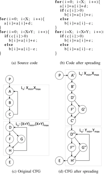
constant and M is a multiplicative coefficient, that can be either a non-negative integer constant, an interval [a,b] or an interval [a,+∞) with both a and b non-negative constants. f o r ( i = 0 ; i <X ; i ++){ a [ i ] = a [ i ] + d ; } f o r ( i = 0 ; i <X+Y ; i ++){ i f ( c [ i ] >0) b [ i ] = a [ i ] + e ; e l s e b [ i ] = a [ i ]− e ; }
(a) Source code
f o r ( i = 0 ; i <X ; i ++){ a [ i ] = a [ i ] + d ; i f ( c [ i ] >0) b [ i ] = a [ i ] + e ; e l s e b [ i ] = a [ i ]− e ; } f o r ( i =X ; i <X+Y ; i ++){ i f ( c [ i ] >0) b [ i ] = a [ i ] + e ; e l s e b [ i ] = a [ i ]− e ; }
(b) Code after spreading
(c) Original CFG (d) CFG after spreading
Fig. 3: The CFG of loop spreading example.
Here, we use the CFG of two loops after the appli-cation of loop spreading as an example to demon-strate the rule. Loop spreading minimizes the parallel execution time by moving some computations from one loop to another. The modifications of source code and the CFG are shown in Figure 3. Figure 3a and Figure 3b give the source code before and after loop spreading, whereas Figure 3c and Figure 3d show their corresponding CFG. In the Figure 3c, basic blocks F and G are the branches in the loop, and an additional constraint is added for them: fF ≥ 2 × fG, which
means that the execution count of F is always no less than twice G. The two loops have different loop bounds and have a dependence (array a is written by the first loop and read by the second loop), so they cannot be fused directly. Loop spreading is needed to move some iterations of loop body of Ly to Lx.
The optimization divides node F into F0 and F00, and same to G. So the rules should be fF → fF0 + fF00 and fG → fG0+ fG00. With the original constraint and rules, we can derive the new constraint fF0+ fF00≥ 2 × (fG0+ fG00).
Another case is the change of a loop bound caused by a compiler optimization. α is a loop bound constraint Lxhlbound, uboundi, with Lx ⊂ original CF G. β
is Lx0hlbound0, ubound0i with Lx0 ⊂ new CF G and lbound0 and ubound0 new loop bounds which should be non-negative integer constants or any expression resulting a non-negative integer.
We still take the loop spreading as the example. In Fig-ure 3, the loop bound of Lyis reduced from X + Y to
Y , so the transformation rule for loop bound should be Lyh(X + Y )min, (X + Y )maxi → LyhYmin, Ymaxi.
With this updated loop bound, we can derive that the execution count of all new basic blocks in this new loop should be no greater than Ymax.
• Removal rule.
This rule is used to express that a basic block or a loop was removed from the CFG by an optimization. Since this rule is never used in the following vectorization optimizations, we will not explain it in detail. More information can be found in [2].
• Addition rule.
This rule is used when any new objects (basic block or loop) are added to the CFG by an optimization. For example, if a new loop LY is introduced into
the new CFG and its loop bounds are known, a new constraint LY hYmin, Ymaxi which involves the new
loop bounds is added.
For each compiler optimization, a set of associated trans-formation rules (change, removal, addition) are defined in agreement to the CFG modifications. When the optimization pass is called, the corresponding rules are applied to transform flow information accordingly.
III. VECTORIZATION AND TRACEABILITY OF FLOW INFORMATION FORWCETCALCULATION
A. Vectorization
Vectorization is a compiler optimization that transforms a scalar implementation of a computation into a vector im-plementation [4], [5]. It consists in processing multiple data at once, instead of processing a single data at a time. All silicon vendors now provide instruction set extensions for this purpose, and usually referred to as single instruction, multiple data (SIMD). Examples of SIMD instruction sets include Intel’s MMX and iwMMXt, SSE, SSE2, SSE3, SSSE3, SSE4.x and AVX, ARM’s NEON technology, MIPS’ MDMX (MaDMaX) and MIPS-3D. The vectorization factor (VF) defines the number of operations that are processed in parallel, and is related to the size of the vector registers supported by the target architecture and the type of data elements. For 128-bit vectors (as in SSE and NEON), and the common types defined by the C language, VF ranges from 2 to 16.
Vectorization is a complex optimization that reorders com-putations. Certain conditions must be met to guarantee the le-gality of the transformation. Parallel loops, where all iterations are independent, can be obviously vectorized. More generally, a loop is vectorizable when the dependence analysis proves that the dependence distance is larger than the vectorization factor. As an example, consider the loops of Figure 4.
• The loop on the left part of the figure is parallel (assuming arrays A and B do not overlap). The data
f o r ( i = 0 ; i <n ; i ++) { A[ i ] =B [ i ] + 2 ; } f o r ( i = 1 ; i <n ; i ++) { A[ i ] =A[ i −1] +2; }
(a) loop-independent (b) loop-carried Fig. 4: No dependence & loop-carried dependence
elements written by an iteration are not written or read by any other iteration. This loop is safe to vectorize. • Conversely, the loop shown on the right part of Figure 4 has a dependence of distance 1: values written at iteration i are read at iteration i+1. Processing these iterations in parallel would violate the dependence, and hence the loop cannot be vectorized.
Compilers usually contain a dependence test to identify the independent operations. For example, LoopVectorizationLegal-ity in LLVM checks for the legality of the vectorization.
Modern vectorization technology includes two methods: Loop-Level Vectorization and Superword Level Parallelism (SLP) [6]. They aim at different optimization situations.
1) Loop-level vectorization: Loop-level Vectorization oper-ates on loops. In the presence of patterns where the same scalar instruction is repeatedly applied to different data elements in a loop, the loop-level vectorizer rewrites the loop with a single vector instruction applied to multiple data. The number that determines the degree of parallelism of data elements is the vectorization factor. Figure 5 is an example of loop vectorization. VF in this example is 4, which means that in the vectorized version, four elements will be processed in one instruction in parallel1. In the meantime, the loop bound is also
divided by 4. Besides, an epilogue loop is created when the loop trip count is not known at compile time to be a multiple of VF, to handle remaining iterations.
Through this example, we can observe that the loop bounds (MAXITER in Figure 5) have changed after vectorization. If the original loop is known to iterate at most N times, the vectorized loop iterates at most M = bN/4c, and the epilogue at most 3 times (V F − 1). Note that keeping the original loop bound for the first loop would be safe, but extremely pessimistic. Not being able to assign a bound to the second loop, however, would make the calculation of the WCET impossible. This toy example shows that flow information will be affected, and this part is the emphasis in the following of this paper.
2) Superword level parallelism: Superword level paral-lelism (SLP) focuses on basic blocks rather than loop nests. It combines similar independent scalar instructions into vector instructions. Consider the example of Figure 6. The three instructions in the function perform similar operations, only the operation elements are different (r, g, b). The SLP vectorizer analyzes these three instructions and their data dependence, and combines them into a vector operation if possible.
The SLP vectorizer first derives the SIMD data width supported by the target architecture. It then checks that the
1Vectorization is performed at the intermediate code level. The example is
given at source code level for readability. In the example A[i : i+3] expresses that the four array elements at indices i to i + 3 are processed in parallel.
f o r ( i = 0 ; i <n ; i ++) / / MAXITER ( N ) { A[ i ] =A[ i ] + 2 ; } f o r ( i = 0 ; i <n −3; i +=4) / / MAXITER (M) { A[ i : i +3]=A[ i : i + 3 ] + 2 ; } f o r ( ; i <n ; i ++) / / MAXITER ( 3 ) { A[ i ] =A[ i ] + 2 ; }
(a) Original source code (b) Vectorized
(V F = 4&M = bN/4c) Fig. 5: Example of loop-level vectorization
t y p e d e f s t r u c t { c h a r r , g , b } p i x e l ; v o i d f o o ( p i x e l b l e n d , p i x e l f g , p i x e l bg , f l o a t a ) { b l e n d . r = a ∗ f g . r + (1− a ) ∗ bg . r ; b l e n d . g = a ∗ f g . g + (1− a ) ∗ bg . g ; b l e n d . b = a ∗ f g . b + (1− a ) ∗ bg . b ; }
Fig. 6: Example of superword level vectorization
statements have the same operations in the same order (mem-ory accesses, arithmetic operations, comparison operations and so on). If so, these statements can be vectorized as long as the data width of the new superword does not exceed the SIMD data width.
Because SLP only focuses on basic blocks, it has no effect on the CFG and the flow information. We transparently handle this optimization in our transformation framework and in the implementation. Thus the rest of this paper focuses on loop-level vectorization.
B. Flow fact traceability for loop-level vectorization
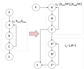
The example of loop-level vectorization expressed at the source code level has been given in Figure 5. The correspond-ing modifications of the CFG are illustrated in Figure 7. In this figure, X in the left part is the loop bound of original Lx
(Xminis the lower bound, whereas Xmaxis the upper bound).
The vectorization factor can be given as an input or decided by the compiler. Through vectorization, the scalar instructions within the loop body B are replaced with the corresponding vector instructions which constitute the new loop body B0.
The example in this figure is a general case. When the loop bound is not known to be a multiple of VF, an epilogue loop is created to process the remaining iterations. Otherwise, the new loop is not needed, or equivalently the loop bound of the new loop is zero. Through the figure, we can observe that the structure of CFG (structure of loops, basic blocks) changes significantly, and the loop bounds of these two loops in the new CFG are also totally different from the original one.
Given the categorization of the transformation rules in Section II-B, this optimization requires the application of both the change rule and the addition rule. The change rule is needed because of the change of the structure and loop bound of loop X. The addition of the new loop requires the addition rule. The set of rules describing the flow transformation of vectorization is given below.
Fig. 7: The CFG of loop-level vectorization example. The left part of the figure shows the original CFG, whereas the right part shows the vectorized one. This CFG corresponds to the code of Figure 5. LXXmin, Xmax →LX bXmin V F c, b Xmax V F c fA→V F × fA0+ fA00 fC→V F × fC0+ fC00 fB→V F × fB0+ fB00 LY h1, V F − 1i
The first line is the change rule that expresses the change of the loop bounds of loop X. The loop bound of the original loop divided by the vectorization factor becomes the new one. The following three lines are change rules. The execution count fA/fB/fC of node A/B/C should be replaced by
V F × fA0/B0/C0+ fA00/B00/C00. The only difference is that the operations in B0 is vector operations, but the ones in A0/C0 are still scalar operations. The final line is an addition rule that expresses the addition of loop bound for the newly created epilogue loop.
To validate the correctness of the transformation rules for vectorization, we have applied them on a large set of benchmarks (those used in Section IV). We have manually verified that the flow information generated by our framework corresponds to the vectorized code generated by the compiler. C. Implementation in the LLVM compiler infrastructure
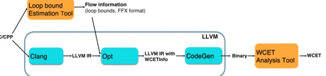
We integrated our framework in the LLVM compiler infras-tructure [7], version 3.3. The LLVM compiler infrasinfras-tructure is designed as a set of modular and reusable compiler and toolchain technologies. As shown in Figure 8, three phases constitute LLVM: Clang (compiler front-end), Opt (LLVM op-timizer) and CodeGen (compiler back-end). Clang is in charge of parsing and validating the C/C++ code and translating it from C/C++ code to the LLVM Intermediate Representation (IR). Opt consists of a series of analyses and optimizations which are performed at IR level. CodeGen produces native machine code.
An important part of the LLVM system is the LLVM Pass Framework. A pass performs an action (transformation, optimization or analysis) on the program.
On Figure 8, there are two external components, depicted as yellow boxes: loop bound estimation tool and WCET esti-mation tool. The former derives loop bounds from the source code. Loop bounds are traced throughout the optimization passes. The WCET estimation tool calculates the WCET from the binary code, in which modified loop bounds have been generated. The input/output format of our framework (portable flow fact expression language FFX [8]) are generic enough to be usable for a large range of loop bound estimation tools and WCET estimations tools.
Theoretically, our transformation framework transforms any flow information expressed as linear constraints. However, for the implementation within LLVM compiler, we focus on tracing only the loop bounds which are the most important information for vectorization.
The loop bounds generated by the loop bound estimation tool are stored in a new object called WCETInfo. WCETInfo is in charge of flow information storage and it is initialized from the source code. It maps loops to the corresponding loop bounds. Different optimizations have different effect on WCETInfo. Each optimization is responsible for updating the map to keep it consistent with its code transformations. Whenever this is too complex, or impossible, an optimiza-tion must delete the WCETInfo object. For superblock level parallelism, we simply preserve WCETInfo because it does not modify loops. For loop-level vectorization, we update WCETInfo according to the transformation rules defined for this optimization.
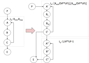
Finally, the code generator CodeGen outputs the final loop bounds to feed the WCET analysis tool for WCET calculation. 1) Specific features of loop-level vectorization in LLVM: Vectorization in LLVM has some specific features that slightly differ from those presented in Section III-B. Actually, LLVM combines vectorization with loop unrolling. When transform-ing flow information, we must thus consider the effect of both transformations.
Loop unrolling replicates the loop body UF times (UF stands for unrolling factor). Loop unrolling is known to reduce the cost of branches and to increase instruction-level parallelism. Unrolling applying jointly with vectorization can also generate more independent instructions. Vectorization as defined in LLVM is depicted in Figure 9.
Compared to Figure 7, the differences are that UF appears, because of the joint application of unrolling and vectorization. The loop body B is replicated V F × U F times for each loop iteration after the vectorization, and the new loop bodies B1. . . BU F are the vector operations transformed from the
original scalar loop body according to the vectorization factor. The transformation rules corresponding to Figure 9 are:
LXXmin, Xmax →LX b Xmin V F × U Fc, b Xmax V F × U Fc fA→(V F × U F ) × fA0+ fA00 fC→(V F × U F ) × fC0 + fC00 fB→V F × (fB1+ . . . + fBU F) + fB00 LY h1, V F × U F − 1i
Fig. 9: The CFG of loop-level vectorization in LLVM. The left part of the figure shows the original CFG, whereas the right part shows the vectorized one.
The first line is also a change rule that expresses the change of the loop bound of loop X. But, here the loop bound of the original loop divided by the product of vectorization factor and unrolling factor becomes the new one. Another difference is about nodes B1. . . BU F. Unlike node A/C, each of these
nodes is the same and contains vector operations, and they are replicated by unrolling. fB should be replaced as V F ×(fB1+ . . . + fBU F) + fB00.
IV. EXPERIMENTS
A. Methodology
Our framework, implemented in the LLVM compiler ver-sion 3.3, traces loop bound information through optimizations, including vectorization. The compiler emits optimized assem-bly code, along with up-to-date loop bounds to characterize all encountered loops. The final part of the process consists in providing the annotated programs to a static WCET analyzer to obtain execution time bounds.
Unfortunately, the WCET estimation tools we have access to (Heptane [9] and Otawa [10]) do not currently support SIMD instruction sets2. We thus relied on measurements on
actual hardware to collect real execution times. Our bench-marks were restricted to single-path programs to guarantee that we are not impacted by path coverage issues. Note that we use measurements only due to the lack of support for SIMD instructions in our WCET estimation tools. Loop bound information is correctly traced through the compiler in all cases.
Execution times in our experiments are measured using the C library function clock(), that returns the number of clock ticks elapsed since the program was launched. We ran each benchmark five times on a completely unloaded system (executing only the operating system and the benchmark under study), and we report the highest observed value. Observed execution times are very stable: the standard deviation for
2We do not foresee any overwhelming difficulty in adding support for
SIMD instructions in WCET estimation tools. However, this was done for time constraints, and left for future work.
C/CPP!
Clang ! LLVM IR!
Flow information!
(loop bounds, FFX format)!
LLVM IR with
WCETInfo! CodeGen! Binary!
Loop bound Estimation Tool!
LLVM!
WCET
Analysis Tool ! WCET! Opt!
Fig. 8: Implementation of traceability of flow information in LLVM
most benchmarks is less than 0.3 s (for the benchmarks whose runtime ranges from 8 s to 50 s) and 1 s (for the benchmarks whose runtime ranges from 50 s to 650 s) on ARM. It is less than 0.03 s (for the benchmarks whose runtime ranges from 1.8 s to 10 s) and 0.1 s (for the benchmarks whose runtime ranges from 10 s to 475 s) on Intel. The observed standard deviations indicate that the operating system activities have no evident effect on the result.
B. Experimental setup
We evaluate the impact of vectorization by using the two following benchmark suites:
• TSVC. TSVC stands for Test Suite for Vectoriz-ing Compilers, developed by Callahan, Dongarra and Levine [11]. It contains 135 loops. It has been ex-tended by the Polaris Research Group at the University of Illinois at Urbana-Champaign [12] and contains 151 loops now. In this paper, we use the modified version included in the LLVM distribution3. We restricted our
experiments to the 112 single-path programs of TSVC. • Gcc-loops. Gcc distributes a set of loops collected on the GCC vectorizer example page4. It is now also one of the LLVM test suites and we can test it in LLVM compiler,5. We restricted our experiments to the 15
single-path programs in this benchmark suite. These two benchmark suites are test suites for vectorizing compilers and as such are loop-intensive programs.
We selected the following two different setups for measur-ing WCETs:
ARM: For the first target, we choose a Panda Board equipped with an OMAP4 ARMv7 processor (v7l) running at 1.2 GHz. It features the advanced SIMD ISA extension NEON. The NEON vectors used in our experiment are 128-bit vectors. The size of L1 instruction cache and data cache are both 32 KB. The size of L2 cache per core is 1 MB. The operating system is Ubuntu 12.04.5. Intel: We also experimented with an Intel
architec-ture: analyses were performed on an Intel Core i7-3615QM CPU with four cores running at 2.30 GHz. The CPU instruction set include ex-tensions SSE4.1 and SSE4.2 (Streaming SIMD
3https://llvm.org/svn/llvm-project/test-suite/trunk/MultiSource/
Benchmarks/TSVC/
4https://gcc.gnu.org/projects/tree-ssa/vectorization.html
5https://llvm.org/svn/llvm-project/test-suite/trunk/SingleSource/UnitTests/
Vectorizer/gcc-loops.cpp
Extensions 4), and AVX. The version used in our experiment is SSE4.2, and the vector size is 128-bit. The size of L1 instruction cache and data cache are both 32 KB. The size of L2 cache per core is 256 KB and L3 cache is 6 MB. The operating system is Mac OS X 10.10.1. Besides, we made sure to turn off Turbo Boost to guar-antee the same execution circumstances for every measurement [13] (Turbo Boost Technology can automatically allow processor cores to run faster than the rated operating frequency if they are operating below power, current, and temperature specification limits).
The Intel Architecture usually is not used in real-time systems. We use it only to denote the effect of vectorization optimizations on different architectures and do not claim it is predictable enough to be used in real-time systems.
In LLVM, VF (vectorization factor) and UF (unrolling factor) can be specified by the user or decided by the compiler. The latter is better in most situations, because they are selected by using a cost model. So in the following experiments, we let LLVM choose VF and UF.
Note that loop vectorization and loop unrolling change the code size and the code memory layout. Thus, on architectures with caches, these optimizations impact both average-case and worst-case performance. This explains the subtle variations of WCETs (mostly positive, but sometimes negative) that we observed and report hereafter.
C. Experimental results
1) Impact of vectorization on WCET: We first measure the WCET obtained with all LLVM optimizations at level -O3 (which enables the vectorizer) for TSVC on ARM and Intel architectures. Then, we evaluate the impact of vector-ization optimvector-ization by manually disabling the vectorvector-ization (-O3 -fno-vectorize) (in this situation loop unrolling is still enabled).
Figures 10 and 11 report on WCET improvements for respectively TSCV on ARM and TSCV on Intel. Reported numbers are the WCET improvement ratios brought by vec-torization (W CETno−vec/W CETvec). There is one bar per
TSVC benchmark; the X-axis gives the number of the bench-mark. Here, not all single-path benchmarks are shown. Only the benchmarks which are affected by vectorization on ARM or Intel architecture are presented. Each figure also reports the average WCET improvement ratio for all benchmarks (including those not affected by vectorization).
It immediately appears that the WCET of many TSVC benchmarks does not improve when turning on vectorization (WCET improvement ratio is 1, hence not shown on figure). This comes from the nature of TSVC, whose objective is to stress vectorizing compilers. Many kernels could simply not be vectorized by LLVM, regardless of our addition for traceability. In those cases, the vectorizer fails, and flow information is simply left unmodified.
a) TSVC and ARM Architecture: Figure 10 shows the impact of vectorization on WCET for the ARM architecture and single-path benchmarks in TSVC.
As mentioned before, not all benchmarks benefit from vectorization. Only a little more than 1/4 of them have a significant WCET improvement ratio, averaging 1.18×.
Theoretically, the WCET improvement ratio could reach 4: these benchmarks manipulate arrays of type float, and the NEON instruction set can operate four elements at the same time. However, the results show that the improvement ratio is around 2 in most cases. The main factors limiting performance are related to the memory subsystem: cache misses and available bandwidth. Vectorized code needs to load four times more data for a similar computational intensity, sometimes reaching the maximum physical bandwidth. And when arrays are larger than a cache level (typically L2 in our benchmarks), frequent cache misses also dominate the performance, limiting the improvement ratio.
We can observe that the WCET improvement ratio of benchmarks s4113 and vas is below 1, i.e. vectorization degrades the WCET. In these two benchmarks, the results of computations are written to memory through an indirection (in the form a[b[i]]=...), a pattern called scatter. LLVM made the decision to vectorize the loop, despite the fact that NEON can only deal with vectors that are stored consecu-tively in memory and cannot vectorize indirect addressing. Additional code is needed for the scatter. Unfortunately, the vectorized loop performs worse that the scalar loop.
b) TSVC and Intel Architecture: We run the same experiments on the Intel architecture. As Figure 11 shows, the LLVM vectorizer results in higher WCET improvement ratio on Intel; the average WCET improvement ratio is 1.41× compared with 1.18× on ARM.
Overall, the WCET improvement ratio due to vectorization is larger on Intel than on ARM. For most benchmarks, the improvement ratio is closer to 4. However, Intel is occasionally impacted by the same factors as ARM. For example, s1111 has a scatter pattern, and necessary scalar instructions limit performance; vag, also has indirect addressing. In s251, s1251 and other similar benchmarks, the performance increase is limited by the cache size: in these benchmarks, the overall size of all accessed arrays is larger than the L2 cache. The improvement ratio of benchmarks s491 and 4117 is below 1, for the same reason as s4113 and vas on ARM: sequences of scalar instructions needed for scatter/gather patterns offset the benefits of vectorization. Finally, the improvement ratio of s176 is above 4: the loop is perfectly vectorized, and LLVM also applied loop unrolling, further increasing performance. We manually disabled loop unrolling and observed that the ratio drops below 4, as expected.
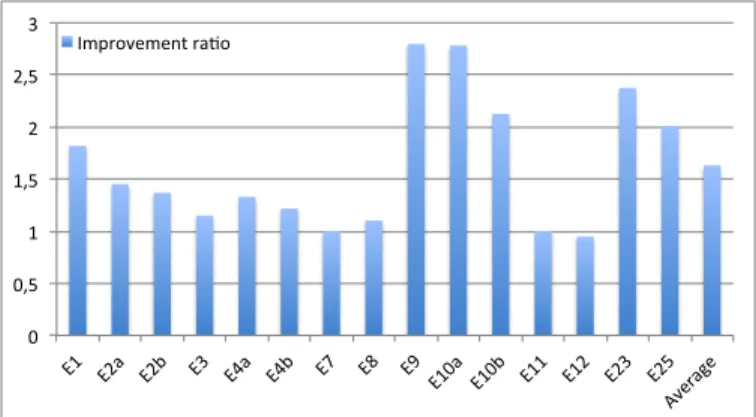
c) Gcc-loops: We measure the WCETs on the single-path codes from Gcc-loops on both Intel and ARM architec-ture. Results are presented on Figure 12 (ARM) and Figure 13
(Intel). As before there is one bar per benchmark in the benchmark suite, and the y-axis gives the WCET improvement ratio obtained when turning on vectorization.
In Figure 13, we can observe that there are 7 benchmarks whose improvement ratio is above 4. Except for E25, the reason for these benchmarks is the same as s176 in TSVC: loop unrolling is applied and increases performance. In the case of E25, the high ratio is also due to a particularly poor sequential code which can be confirmed with the Intel Architecture Code Analyzer [14]: the generated sequential code results in many more micro-operations than the vectorized loop.
Through these figures, we can make similar observations as on TSVC. Vectorization reduces WCETs, and does this more effectively on Intel architecture.
0 0,5 1 1,5 2 2,5 3 E1 E2a E2b E3 E4a E4b E7 E8 E9 E10a E10b E11 E12 E23 E25 Averag e Improvement ra:o
Fig. 12: Impact of vectorization on WCET (ARM, single-path Gcc-loops) 0 1 2 3 4 5 6 7 8 E1 E2a E2b E3 E4a E4b E7 E8 E9 E10a E10b E11 E12 E23 E25 Averag e Improvement ra:o
Fig. 13: Impact of vectorization on WCET (Intel, single-path Gcc-loops)
V. RELATED WORK
WCET estimation methods have been the subject of sig-nificant research in the last two decades (see [1] for a survey). Comparatively less research was devoted to WCET estima-tion in the presence of optimizing compilers. Early research was first presented by Engblom et al. [15]. They propose an approach to derive WCET when code optimizations are applied. Compared with their not powerful structure, we can handle most LLVM optimizations, including vectorization.
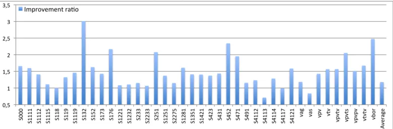
0,5 1 1,5 2 2,5 3 3,5 S0 00 S1 11 1 S1 11 2 S1 11 5 S1 18 S1 19 S1 11 9 S1 32 S1 52 S1 73 S1 76 S1 22 1 S1 23 2 S2 33 S2 23 3 S2 51 S1 25 1 S2 27 5 S1 28 1 S1 35 1 S1 42 1 S4 23 S4 31 S4 52 S4 71 S4 91 S4 11 2 S4 11 3 S4 11 4 S4 11 7 S4 12 1 vag vas vp v vtv vp vtv vp vts vp vp v vtv tv vb or Av er ag e Improvement ra<o
Fig. 10: Impact of vectorization on WCET (ARM, single-path TSVC benchmarks). The y-axis represents the WCET improvement ratio brought by vectorization: W CETno−vec/W CETvec.
0,5 1 1,5 2 2,5 3 3,5 4 4,5 S0 00 S1 11 1 S1 11 2 S1 11 5 S1 18 S1 19 S1 11 9 S1 32 S1 52 S1 73 S1 76 S1 22 1 S1 23 2 S2 33 S2 23 3 S2 51 S1 25 1 S2 27 5 S1 28 1 S1 35 1 S1 42 1 S4 23 S4 31 S4 52 S4 71 S4 91 S4 11 2 S4 11 3 S4 11 4 S4 11 7 S4 12 1 vag vas vp v vtv vp vtv vp vts vp vp v vtv tv vb or Av er ag e Improvement ra<o
Fig. 11: Impact of vectorization on WCET (Intel, single-path TSVC benchmarks). The y-axis represents the WCET improvement ratio brought by vectorization: W CETno−vec/W CETvec.
Later, Kirner et al. [16], [17] present a method to transform flow information from source code level to machine code level. The SATIrE [18] system is designed as a source-to-source analysis tool to map source-to-source code annotations to the intermediate program representation. Then it is used to build a WCET analysis tool by Barany et al. [19]. This tool can transform the flow information in the source code level to the WCET analysis on different levels. These methods all rely on source-to-source transform, while we focus on traceability within the compiler, down to the code generator.
Raymond et al. [20] integrate an existing verification tool to check the improvement of the estimated WCET from high-level model to C, and then binary code. Our work not only is intended to complement theirs, but also focuses on vectorization now.
Huber et al. [21] propose an approach based on a new representation: control flow relation graph. Their approach relates intermediate code and machine code when generating machine code in compiler back-ends. In contrast to them, we focus on optimizations including vectorization performed at the intermediate code level.
Finally, the framework [2] proposed by Li et al., that served as a basis for this paper, provides a method to trace and maintain flow information from source code to machine code even with compiler optimizations.
Our research has similar objectives than all these previous work, but to our best knowledge, no previous work was able to trace vectorization in optimizing compilers.
Another related research is WCC6. WCC (WCET-aware compilation) focuses on the optimizations for WCET mini-mization instead of ACET minimini-mization.
In our work, we do not aim at defining optimizations that decrease the WCET. Instead, we are using standard optimizing compilers, that optimize ACET, and focus on traceability of flow information.
The performance of vectorization has been studied ex-tensively. Maleki et al. [22] evaluate three main vectorizing
6http://ls12-www.cs.tu-dortmund.de/daes/en/forschung/
compilers: GCC, the Intel C compiler and the IBM XLC com-piler. They evaluate how well these three compilers vectorize benchmarks and applications. The introduction and evaluation of vectorization optimization in LLVM is presented in [23]. That document introduces the usage of vectorizers in LLVM through examples, and gives performance numbers of the LLVM vectorizer on benchmark gcc-loops as compared to GCC. Further evaluation of vectorization is given by Finkel in [24]. In this document, the benchmark TSVC is used to test the vectorization with LLVM as compared to the GCC vectorizer.
Compared with the above documents, we focus on the WCET as a performance metric instead of average-case per-formance. Except our work, to our best knowledge there is no work studying the impact of vectorization on WCET.
VI. CONCLUSION
Designers of real-time systems must compute the WCET of the various interacting tasks to guarantee that they all meet their deadlines. Computed WCET bounds must be safe. To avoid over-provisioning systems, they should also be tight. High level flow information helps producing tight estimates. Unfortunately, this information is difficult to trace through complex compiler optimizations, and designers often prefer disabling optimizations.
Vectorization has become a mature and powerful optimiza-tion technique that can deliver significant speedups. However, it severely impacts the control flow of the program, making traceability of flow information challenging, and it is therefore not used in real-world systems.
In this paper we proposed an approach to trace flow information from source code to machine code through an existing implementation of vectorization. When the vectorizer changes the structure of CFG, the flow information available at source code level is maintained and updated, such that the final WCET analyzer has enough information for the WCET calculation. We implemented this framework in LLVM compiler. Experimental results with measured WCETs show that vectorization is highly beneficial for real-time systems as well: we are able to improve WCET, on average by 1.18× on ARM/NEON and 1.41× on Intel SSE on a benchmark suite designed for vectorizing compilers (TSVC).
Integrating support for SIMD instruction sets in WCET estimation tools is part of our future work. Another direction for future work is to implement the traceability mechanisms such that portability to a different compiler or to different compiler versions is eased.
REFERENCES
[1] R. Wilhelm, J. Engblom, A. Ermedahl, N. Holsti, S. Thesing, D. Whal-ley, G. Bernat, C. Ferdinand, R. Heckmann, T. Mitra, F. Mueller, I. Puaut, P. Puschner, J. Staschulat, and P. Stenstr¨om, “The worst-case execution-time problem–overview of methods and survey of tools,” ACM Trans. Embed. Comput. Syst., vol. 7, no. 3, pp. 36:1–36:53, 2008. [2] H. Li, I. Puaut, and E. Rohou, “Traceability of flow information: Reconciling compiler optimizations and wcet estimation,” in RTNS-22nd International Conference on Real-Time Networks and Systems, 2014.
[3] Y.-T. S. Li and S. Malik, “Performance analysis of embedded software using implicit path enumeration,” IEEE Trans. on CAD of Integrated Circuits and Systems, vol. 16, no. 12, pp. 1477–1487, 1997. [4] D. Naishlos, “Autovectorization in GCC,” in Proceedings of the 2004
GCC Developers Summit, 2004, pp. 105–118.
[5] E. Rohou, K. Williams, and D. Yuste, “Vectorization technology to improve interpreter performance,” ACM Trans. Archit. Code Optim., vol. 9, no. 4, pp. 26:1–26:22, Jan. 2013.
[6] S. Larsen and S. Amarasinghe, Exploiting superword level parallelism with multimedia instruction sets. ACM, 2000, vol. 35, no. 5. [7] C. Lattner and V. Adve, “LLVM: A compilation framework for lifelong
program analysis and transformation,” in Int’l Symp. on Code Gener-ation and OptimizGener-ation (CGO), San Jose, CA, USA, Mar. 2004, pp. 75–88.
[8] J. Zwirchmayr, A. Bonenfant, M. de Michiel, H. Cass´e, L. Kovacs, and J. Knoop, “FFX: A Portable WCET Annotation Language,” in Int’l Conference on Real-Time and Network Systems (RTNS), 2012, pp. 91– 100.
[9] A. Colin and I. Puaut, “Worst case execution time analysis for a processor with branch prediction,” Real-Time Systems, vol. 18, no. 2-3, pp. 249–274, 2000.
[10] C. Ballabriga, H. Cass, C. Rochange, and P. Sainrat, “Otawa: An open toolbox for adaptive wcet analysis,” in Software Technologies for Embedded and Ubiquitous Systems, ser. Lecture Notes in Computer Science. Springer Berlin Heidelberg, 2010, vol. 6399, pp. 35–46. [11] D. Callahan, J. Dongarra, and D. Levine, “Vectorizing compilers: A test
suite and results,” in Proceedings of the 1988 ACM/IEEE conference on Supercomputing. IEEE Computer Society Press, 1988, pp. 98–105. [12] Polaris Research Group, University of Illinois at Urbana-Champaign, “Extended test suite for vectorizing compilers,” http://polaris.cs.uiuc. edu/∼maleki1/TSVC.tar.gz.
[13] L. Emurian, A. Raghavan, L. Shao, J. M. Rosen, M. Papaefthymiou, K. P. Pipe, T. F. Wenisch, and M. M. K. Martin, “Pitfalls of accurately benchmarking thermally adaptive chips,” in Workshop on Duplicating, Deconstructing, and Debunking (WDDD), Jun. 2014.
[14] Intel Architecture Code Analyzer – User’s Guide, 2nd ed., Intel Corpo-ration, 2013.
[15] J. Engblom, A. Ermedahl, and P. Altenbernd, “Facilitating worst-case execution times analysis for optimized code,” in Euromicro Workshop on Real-Time Systems, 1998, pp. 146–153.
[16] R. Kirner, “Extending optimising compilation to support worst-case execution time analysis,” Ph.D. dissertation, Technische Universit¨at Wien, 2003.
[17] R. Kirner, P. Puschner, and A. Prantl, “Transforming flow information during code optimization for timing analysis,” Real-Time Systems, vol. 45, no. 1, pp. 72–105, 2010.
[18] M. Schordan, “Source-to-source analysis with SATIrE - an example revisited,” in Scalable Program Analysis, ser. Dagstuhl Seminar Pro-ceedings, no. 08161. Dagstuhl, Germany: Schloss Dagstuhl - Leibniz-Zentrum fuer Informatik, Germany, 2008.
[19] G. Barany and A. Prantl, “Source-level support for timing analysis,” in Conference on Leveraging Applications of Formal Methods, Verifica-tion, and ValidaVerifica-tion, 2010, pp. 434–448.
[20] P. Raymond, C. Maiza, C. Parent-Vigouroux, and F. Carrier, “Timing analysis enhancement for synchronous program,” in Int’l Conference on Real-Time and Network Systems (RTNS), 2013, pp. 141–150. [21] B. Huber, D. Prokesch, and P. Puschner, “Combined WCET analysis
of bitcode and machine code using control-flow relation graphs,” in Conference on Languages, Compilers and Tools for Embedded Systems (LCTES), 2013, pp. 163–172.
[22] S. Maleki, Y. Gao, M. J. Garzaran, T. Wong, and D. A. Padua, “An evaluation of vectorizing compilers,” in Parallel Architectures and Compilation Techniques (PACT), 2011 International Conference on. IEEE, 2011, pp. 372–382.
[23] “Auto-vectorization in LLVM,” http://llvm.org/docs/Vectorizers.html. [24] H. Finkel, “Autovectorization with LLVM,” http://llvm.org/devmtg/