HAL Id: hal-00605568
https://hal.archives-ouvertes.fr/hal-00605568
Submitted on 2 Jul 2011
HAL is a multi-disciplinary open access
archive for the deposit and dissemination of
sci-entific research documents, whether they are
pub-lished or not. The documents may come from
L’archive ouverte pluridisciplinaire HAL, est
destinée au dépôt et à la diffusion de documents
scientifiques de niveau recherche, publiés ou non,
émanant des établissements d’enseignement et de
Adjunctions on the lattice of dendrograms and
hierarchies
Fernand Meyer
To cite this version:
Adjunctions on the lattice of dendrograms and
hierarchies
Fernand Meyer
July 2, 2011
Abstract
Morphological image processing uses two types of trees. The min-tree represents the relations between the regional minima and the various lakes during ‡ooding. As the level of ‡ooding increases in the various lakes, the ‡ooded domain becomes larger.
A second type of tree is used in segmentation and is mainly associ-ated to the watershed transform. The watershed of a topographic surface constitutes a partition of its support. If the relief is ‡ooded, then for in-creasing levels of ‡oodings, catchment basins merge. The relation of the catchment basins during ‡ooding also obeys a tree structure.
We start by an axiomatic de…nition of each type of tree, min and max tree being governed by a single axiom ; for nested catchment basins, a second axiom is required.
There is a one to one correspondance between the trees and an ultra-metric half distance, as soon one introduces a total order compatible with the inclusion.
Hierarchies obey a complete lattice structure, on which several adjunc-tions are de…ned, leading to the construction of morphological …lters.
Hierarchies are particular useful for interactive image segmentation, as they constitute a compact representation of all contours of the image, structured in a way that interesting contours are easily extracted.
The last part extends the classical connections and partial connections to the multiscale case and introduces taxonomies.
1
Introduction
Hierarchies are the classical structure for representing a taxinomy. The most famous taxonomy, the Linnaean system classi…ed nature within a nested hier-archy, starting with three kingdoms. Kingdoms were divided into Classes and they, in turn, into Orders, which were divided into Genera (singular: genus), which were divided into Species (singular: species). Below the rank of species he sometimes recognized taxa of a lower (unnamed) rank (for plants these are now called "varieties").
Hierarchies are also useful in the domain of image processing. In the …eld of mathematical morphology, two basic hierarchies appear. The …rst is the min-tree structuring the successive lakes of a ‡ooding and its dual counterpart, the max-tree. It has been introduces by Ph.Salembier [8] as a useful condensation of information and support of powerful image …ltering methods, based on the pruning of branches of this tree. During ‡ooding, lakes grow and merge ; the ‡ooded area also becomes larger, but does not necessarily occupy the whole domain.
Hierarchies are also at the core of hierarchical segmentation, as they repre-sent in a condensed way nested partitions obtained through image segmentation. Hierarchies appear quite naturally in the …eld of morphological segmentation, which uses as tool the watershed of gradient images. As a matter of fact, the catchment basins of a topographic surface form a partition. If a basin is ‡ooded and does not contain a regional minimum anymore, it is absorbed by a neigh-boring basin and vanishes from the segmentation. A hierarchy is hence obtained by considering the catchment basins associated to increasing degrees of ‡ood-ing, producing for each particular ‡ooding a partition. For increasing ‡oodings, the partitions become coarser and are nested. They structure the image into a multiscale representation ; the nested partitions permit to weight the contours : the importance of a contour being measured by the level of the hierarchy where it disappears [4].
Both types of tree share a common structure, that of a tree. However they di¤er by their support : successive lakes while ‡ooding a relief do not cover the complete domain of the relief ; furthermore the covered area increases as the lakes grow higher. On the other hand, the catchment basins of this same relief associated to the successive ‡oodings all partition the domain of the relief. In the …rst case, we speak of dendrogram or partial hierarchy, in the second case of hierarchy or covering hierarchy.
Often one is not interested in partitioning the total domain of the image, but one wants to get the masks of some objects of interest. These masks are disjoint sets but do not partition the domain ; they constitute a partial partition as introduced by Ch. Ronse [5]. The paper is organized as follows.
The …rst part starts with the axiomatic de…nition of trees, dendrograms and hierarchies due to Benzecri [2]. Dendrograms are based solely on the intersection axiom and correctly model min and max-trees. Hierarchies are obtained by adding a second axiom, the union axiom.
We show in this paper, that this second axiom very often is not necessary and that most useful properties derive from the intersection axiom alone. Adding the union axiom obliges …lling the empty spaces left by an operator like an erosion applied to a hierarchy ; in contrast, the intersection axiom alone allows an automatic adjustment of the support during the erosion.
Dendrograms may be further structured by adding a complete preorder re-lation, compatible with inclusion order, called strati…cation level. Strati…ed hierarchies are the basis of taxonomy. A partial ultrametric distance is then associated to each couple (dendrogram, strati…cation).
The fourth part de…nes two adjunctions on partial hierarchies. The …rst extends the adjunction de…ned by J.Serra for partitions [11], where each tile of a partition is eroded and dilated separately, empty spaces being …lled with singletons. Ch. Ronse described the adjoint dilation [6] and also adapted this de…nition to partial partitions, where the empty spaces are kept outside of the support of the result [7]. We extend the adjunction de…ned by J.Serra and Ch. Ronse to partial hierarchies. As the support of partial hierarchies and dendrograms may vary, the de…nition of erosions and dilations is easier on a dendrogram as on a hierarchy.
We also de…ne a second adjunction which directly relies on the complete lattice structure of PUHD. The supremum of translated PUHD yields the ero-sion by a structuring element equal to the set of translations ; the in…mum of translated PUHD yields the dilation. This second adjunction is …ner than the …rst.
In a …fth part, we show how some interactive segmentation tools may be derived from a hierarchy.
The last part of the document extends the connections de…ned for partitions to hierarchies and de…nes taxonomies. The algebraic structure of partitions has been studies by Serra, Heijmans, Ronse ([3], [12], [7]). The same set may be par-titioned into distinct partitions according the type of connectivity one adopts. Serra has laid down the adequate framework for extending the topological no-tion of connectivity by de…ning connective classes later called connecno-tions ( [10], [12]). Taxonomies, like connections are generated by the union of sets with a non empty intersection ; a taxonomy class possesses an strati…cation index, which can be interpreted as the diameter for an ultrametric distance. The diameter of a family of sets with an empty intersection being the largest diameter of a set in the family. Connected classes are then simply the sets with diameter 0 for a binary ultrametric distance.
2
Dendrograms
The axiomatic de…nition of dendrograms and hierarchies is due to Benzecri [2]. It entirely relies on set intersection or union and on the inclusion order relation between sets. The construction is very progressive : starting with the inclusion order relation alone and adding axioms in order to successively de…ne trees, hierarchies and …nally strati…ed hierarchies.
2.1
The structure associated to an order relation
Let E be a domain whose elements are called points. Let X be a subset of P(E), on which we consider an arbitrary order or preorder relation relation (the inclusion between sets is an example, but what follows is valid for any preorder relation). The union of all sets belonging to X is called support of X : supp(X ): The subsets of X may be structured into:
the leaves : Leav(X ) = fA 2 X j 8B 2 X : B A ) A = Bg the nodes : Nod(X ) = X Leav(X )
the predecessors : Pred(A) = fB 2 X j A Bg the immediate predecessors :
ImPred(A) = fB 2 X j fU j U 2 X ; A U and U Bg = (A; B)g the successors : Succ(A) = fB 2 X j B Ag
the immediate successors :
ImSucc(A) = fB 2 X j fU j U 2 X ; B U and U Ag = (A; B)g The leaves are disjoint sets ; so are also the summits. The summits of X constitute a partition of supp(X ). This is not necessarily the case of the leaves : a set B A may be a leave, but the remaining points of A do not necessarily belong to a leave. It will only be the case if the union axiom is satis…ed, yielding covering hierarchies (see below).
The leaves are successors of the summits and local minima ; the summits are predecessors of the leaves and local maxima. The name predecessor and successor supposes that one explores the …liations between nodes in a direction going from the summits to the leaves, from coarse to …ne.
2.2
Dendrograms
We now structure X as a tree or a dendrogram. We also use "partial hierarchy" as an alternative name for dendrogram.
Dendrograms : X is a dendrogram if and only if the set Pred(A) of the predecessors of A; with the order relation induced by is a total order. The maximal element of this family is a summit, which is the unique summit con-taining A:
There exist several equivalent characterization of dendrograms which are instructive.
Nota bene: From now on we take as preorder relation on P(E) the ordinary inclusion between sets.
Proposition 1 The following properties are equivalent: 1)X is a dendrogram
2) U; V; A 2 X : A U and A V ) U V or V U 3) U; V 2 X : U " V and V " U ) U \ V = ?
Proof.
1) ) 2) : Suppose that X is a dendrogram, i.e. for all A 2 X : Pred(A) is completely ordered for
U; V; A 2 X : A U and A V means that U 2 Pred(A) and V 2 Pred(A) and since Pred(A) is completely ordered for ; we have U V or V U 2) ) 3) : Suppose now that U; V; A 2 X : A U and A V ) U V or
V U: This implication is equivalent with the following where each predicate has been negated:
U; V 2 X : U " V and V " U ) @A 2 X : A U and A V But this last predicate implies that U \ V which is included both in U and in V is empty : U \ V = ?
3) ) 2) : Suppose that U; V 2 X : U " V and V " U ) U \ V = ? ; inverting the predicates yields the equivalent implication U \ V 6= ? ) U V or V U: But then if there exists A such that A U and A V; it means that U \ V 6= ? implying U V or V U
2) ) 1) : Suppose now that U; V; A 2 X : A U and A V ) U V or V U: Consider a set A and two sets U; V 2 Pred(A): This means that A U and A V; implying that U V or V U; showing that Pred(A) is indeed well ordered.
Proposition 2 A family (Ai)i2I of sets in X with a non empty intersection is
completely ordered for : Proof.
Suppose that there exists a set U included in each Ai: We may then apply
the criterion 2 characterizing dendrograms to any couple Aj; Ak showing that
Aj Ak or Ak Aj and that the family (Ai)i2I is completely ordered for :
Consider now a point p belonging to supp(X ); i.e. there exists a set A 2 X such that p 2 A: The set fpg is included in the family of all sets of X containing p: This family is thus completely ordered for and contains a smallest element, which we call home(p). We call Pred(p) the set of predecessors of home(p) : Pred(p) = Pred(home(p))
2.2.1 Representation of a dendrogram as a tree
In the case where X is …nite, then X is a dendrogram if and only if any element A 2 X Sum(X ) possesses a unique immediate predecessor.
A dendrogram is said to be connected if it possesses a unique summit : Card Sum(X ) = 1
Finite dendrograms are classically represented as a tree : each element A 2 X is a node of the tree, and is linked by an edge with its unique immediate predecessor.
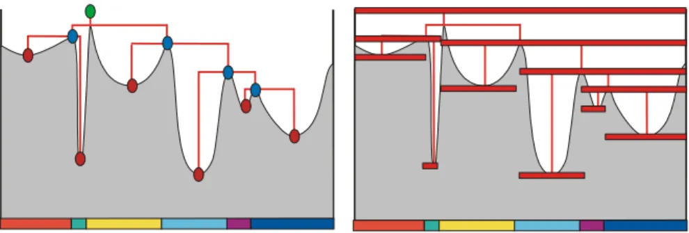
Consider the topographic surface represented in …g.1, ‡ooded by a ‡ood of uniform altitude. As the altitude increases, lakes appear at the position of the regional minima and progressively …ll the catchment basins. When the lowest pass point of a catchment basin is reached, two neighboring lakes merge, forming a new lake. The mintree [8] represents the evolution of the lakes during ‡ooding. Each lake is represented as a node : the leaves are the lakes as they appear at the location of the regional minima and are represented as red dots. The lakes created by merging of two preexisting lakes are represented as blue dots. Finally, the unique lake which covers everything is the root of the tree
Figure 1: Left : the mintree of a topographic surface. The horizontal mosaic image at the bottom represents the extension of the catchment basins of the relief.
Right : A hierarchy associated to the mintree : each node of the mintree is replaced on the catchment basins of the relief associated to all successors of this node. The altitude of each region represents one possible strati…cation of this hierarchy
Figure 2: Partial hierarchy of the critical lakes, i.e. the lakes appearing at the minima or the lakes which immediately resulted from the fusion of two smaller lakes.
and is represented as a green dot. Each node, except the summit is linked by an edge with its unique predecessor, the lake formed by merging with another lake. The catchment basins of the relief are represented as coloured mosaic at the bottom of the relief.
We may now associate two distinct families of sets belonging to P(E): The …rst one is represented in the right part of …gure 1, where each node has been replaced by the union of catchment basins which cut the corresponding minimum or lake. In this case, as one goes down the hierarchy, the regions split but constitute a partition of the domain. The second is represented in …g.2, where each node is replaced by the regional minimum or the lake created at this node. In this second case, as one goes down the hierarchy, the domain covered by the lakes or the minima becomes smaller and smaller. In the binary case, there are only one level : disjoint sets cover the domain E; and constitute a partition. Alternatively, they are disjoint but without covering E; then they constitute a partial partition.
2.2.2 Partitions and partial partitions
Consider a dendrogram verifying : A 2 supp( ) ) Pred(A) = A: Such a dendrogram is called partial partition (partial partitions have been introduced by Ch. Ronse in [5]). If supp( ) = E; then it is called partition.
Let U; V 2 and U 6= V . As Pred(U) = U and Pred(V ) = V we necessarily have U " V and V " U , implying according criterion 3 of dendrograms that U \ V = ?:
Inversely consider a subset of P(E) such that any two sets U; V 2 verify U = V or U \V = ?: Consider now two sets A; B2 such that B 2 Pred(A): As A B; we have A \ B 6= ?; leaving as only possibility A = B; showing that Pred(A) = A:
3
Strati…cation indices and ultrametric half
dis-tances
The collection of regions depicted in red in the right part of …g.1 obviously rep-resents a dendrogram: the region at each node is included in all its predecessors. This partial order relation governs the hierarchical structure of the tree. This inclusion order can be made more precise, by the adjunction of a total order compatible with it.
Such a …ner partial order between the regions has been introduced in …g.1, where each catchment basin is represented at the altitude of the ‡ooding for which this catchment basin appears for the …rst time. If a catchment basin is included in another, the its altitude where the …rst appears is smaller than the altitude where it gets absorbed by the second. For this reason, we say that the altitude constitutes a total order between the catchment basins compatible with the partial inclusion order. We call it a strati…cation index of the hierarchy. All
nodes with the same altitude represent a strati…cation level of the hierarchy. Let us de…ne precisely what we mean by strati…cation index.
3.1
Strati…cation index
X is a strati…ed dendrogram (or partial hierarchy), if it is equipped with an index function st from X into the interval [0; L] of R which is strictly increasing with the inclusion order:
8A; B 2 X : A B and B 6= A ) st(A) < st(B):
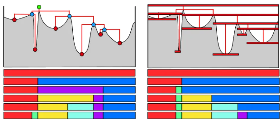
It will be useful to set st(?) = L: We suppose that for all A 2 X : st(A) < L: There are many strati…cation indices compatible with a given hierarchy. Fig.3 presents two strati…cation indices compatible with the same dendrogram: On the left, we consider the watershed segmentation if one takes as marker the minima, ordered by their altitude. The coarsest level covers the domain. The next level is associated to the two lowest minima taken as markers. The successing levels progressively introduce more minima until all minima are used as markers, cyielding the …nest segmentation.
On the right, the coarsest and …nest segmentations are the same, in between we consider a ‡ooding with uniform and growing altitude over the domain E: As lakes merge, cachment basins also merge.
This example shows two radically di¤erent strati…cation indices, that is total order, compatible with the partial order induced by inclusionf of sets expressed by the dendrogram.
3.1.1 Extremal strati…cation indices
Among all possible strati…cation indices compatible with a hierarchy, there exist two extremal strati…cation indices.
The largest strati…cation index assigns the maximal value L to the summits and decreases as one goes down to the successors. The smallest strati…cation level assigs 0 to alll leaves and increases as one goes up along the predecessors of the leaves.
If the hierarchy X is …nite, the maximal and minimal strati…cation levels may be computed as follows.
Maximal strati…cation : st(summits) = L 8A 2 X : st(A) = st(ImPred(A)) 1 Minimal strati…cation : st(Leaves) = 0 8A 2 X : st(A) = st(ImSucc(A)) + 1
Any linear combination between the maximal and minimal strati…cation is still a valid strati…cation.
Figure 3: Two strati…cation indices compatible with the same dendrogram: On the left, we consider the watershed segmentation if one takes as marker the minima, ordered by their altitude. The coarsest level covers the domain. The next level is associated to the two lowest minima taken as markers. The successing levels progressively introduce more minima until all minima are used as markers, cyielding the …nest segmentation.
On the right, the coarsest and …nest segmentations are the same. Here we consider a ‡ooding with uniform and growing altitude over the domain E: As lakes merge, cachment basins also merge. The order of merging is however quite di¤erent from the left …gure.
3.2
A partial ultrametric distance associated to each
den-drogram
De…nition 3 is a partial ultrametric distance as: 8p; q 2 E : (p; q) = (q; p)
8p; q; r 2 E : (p; q) max f (p; r); (r; q)g
Proposition 4 Each dendrogram X with a strati…cation index st induces on the points of E a partial ultrametric distance de…ned as follows:
for p; q 2 E; p =2 supp(X ) : (p; p) = L and (p; q) = L
for p; q =2 supp(X ) : if no set of X contains both p and q; then (p; q) = L: for p; q 2 supp(X ) : let A be a set of X containing both p and q: Thus the family (Ai)i2I of sets of X containing both p and q is not empty and has a
non empty intersection ; as established above is completely ordered for and possesse a smallest element. The distance (p; q) is the strati…cation level of the smallest set in this family.
Proof. Let us prove that indeed is a partial ultrametric distance. The symmetry is obvious.
a) if r =2 supp(X ); then (p; r) = (r; q) = L and the ultrametric inequality holds
b) p or q does not belong to supp(X ), say p : then (p; q) = (p; r) = L and the ultrametric inequality holds
c) p; q; r 2 supp(X ) :
(p; r) is the strati…cation index of a set A1 2 X containing p and r: Hence
A12 Pred(r)
Similarly (r; q) is the strati…cation index of a set A2 2 X containing q and r
and belongs to Pred(r):
But Pred(r) is well ordered for ; hence A1 A2or A2 A1
Suppose A1 A2: then A2is the smallest set of Pred(r) containing r and q; but
also contains p: Hence (p; q) (r; q) = st(A2) since (p; q) is the strati…cation
index of the smallest set of X containing both p and q:
This last inequality is called ultrametric inequality, it is stronger than the triangular inequality.
De…nition 5 For p 2 E the closed ball of centre p and radius is de…ned by Ball(p; ) = fq 2 E j (p; q) g : The open ball of centre p and radius is de…ned by Ball(p; ) = fq 2 E j (p; q) < g :
Remark 6 Every triangle in a domain where an ultrametric distance is de…ned is isosceles. Let us consider three distinct points p; q; r and suppose that the largest edge of this triangle is pq: Then d(p; q) d(p; r) _ d(r; q); showing that the two larges edges of the triangle have the same length.
3.2.1 Properties of the balls of a partial ultrametric distance Lemma 7 Each element of a closed ball Ball(p; ) is centre of this ball Proof. Suppose that q is an element of Ball(p; ). Let us show that then q also is centre of this ball. If r 2 Ball(p; ) : (q; r) max f (q; p); (p; r)g = ; hence r 2 Ball(q; ); showing that Ball(p; ) Ball(q; ): Exchanging the roles of p and q shows that Ball(p; ) = Ball(q; )
Lemma 8 Two closed balls Ball(p; ) and Ball(q; ) with the same radius are either disjoint or identical.
Proof. If Ball(p; ) and Ball(q; ) are not disjoint, then they contain at least one common point r: According to the preceding lemma, r is then centre of both balls Ball(p; ) and Ball(q; ), showing that they are identical.
Lemma 9 The radius of a ball is equal to its diameter.
Proof. Let Ball(p; ) be a ball of diameter ; that is the maximal distance between two elements of the ball is . Thus : Let q and r be two extremities of a diameter in Ball(p; ) : = (q; r) (q; p) _ (p; r) = : Hence = : Remark 10 Instead of closed balls, we could have taken open balls. The results are the same.
3.2.2 Typology of the points of E
Partial hierarchy A strati…ed dendrogram X structures the domain E into various categories of points :
- a point p is an alien if p =2 supp(X ); for such a point that (p; p) = L - a point p is a singleton if p 2 supp(X ) and home(p) = fpg ; for such a point : (p; p) < (p; q) for q 6= p
- all other points of supp(X ) are regular points of X
Due to the ultrametric inequality, we also have (p; p) (p; q) _ (q; p) = (p; q): Hence (p; p) V
q6=p
(p; q):
Partial partitions We de…ne aliens and singletons of a partial partition : Singletons are characterized by: 8p; q 2 E ; p 6= q; : (p; q) = 1 and
(p; p) = 0:
Aliens are characterized by: 8p 2 E : (p; p) = 1 implying 8p; q 2 E : (p; q) = 1
the support of is the set of points p verifying : (p; p) = 0
3.3
Inversely: a dendrogram associated to each partial
ultrametric distance
Consider now a partial ultrametric distance :
Proposition 11 The closed balls of a partial ultrametric distance form a dendrogram X
Proof.
We have to show that for any set A belonging to X , Pred(A) is well ordered for :
Consider two sets B1 = Ball(p; ) and B2 = Ball(q; ) containing both A: We
have to show that they are comparable for :
Let r be a point of A. This point belongs to both Ball(p; ) and Ball(q; ); hence it is centre of each of these balls : Ball(p; ) = Ball(r; ) and Ball(q; ) = Ball(r; ): If = ; then Ball(p; ) and Ball(q; ) are identical. If < ; then Ball(p; ) = Ball(q; ). This establishes that Pred(A) is well ordered for Proposition 12 We have a one to one correspondance between partial ultra-metric distances and strati…ed dendrograms X
4
Partial partitions
Consider a dendrogram verifying : A 2 supp( ) ) Pred(A) = A: Let us verify that such a dendrogram is a partial partition, as they have been called by Ch. Ronse in [5].
Its partial ultrametric distance is now a binary, taking its values in f0; 1g : It veri…es
(pp1) : for p; q; r 2 supp( ) : (p; q) = (q; p) (q; r) _ (r; p) : sym-metry and ultrametric inequality
(pp2) for p =2 supp( ); 8q 2 E : (p; q) = 1
This last relation is also true for p itself : for p =2 supp( ) : (p; p) = 1 The domain supp( ) = fp 2 E : (p; p) = 0g is called support of the partial partition. If this domain equals E; then is a partition. Otherwise is a partial partition.
Consider now a point p =2 supp( ): We call such points "aliens". For any q 2 E; we have 1 = (p; p) (p; q) _ (q; p) = (p; q); showing that the ultrametric distance between an alien and any other point is 1:
Remark 13 Aliens should not be mixed up with the singletons, which duly be-long to the support. The singleton fxg is a set of P(E) reduced to the point x: Singletons are characterized by: 8q 2 E ; p 6= q; : (p; q) = 1 and (p; p) = 0:
We call cl(p) the closed ball of centre p and of radius 0 associated to : Relation (pp2) implies that for p =2 supp( ) the class cl(p) is empty.
Consider now p; q 2 E such that q 2 cl(p). This shows that p; q 2 supp( ) and (p; q) = 0: If r 2 cl(p); then (p; r) = 0 and (q; r) (q; p) _ (p; r) = 0 showing that r 2 cl(q): Similarly r 2 cl(q) ) r 2 cl(p):
Hence for any p; q 2 E ; q 2 cl(p) ) cl(q) = cl(p):
But these are precisely the criteria given by Ch. Ronse for de…ning partial partitions:
(P1b) for any p 2 E ; cl(p) = ? or p 2 cl(p) (P2a) for any p; q 2 E ; q 2 cl(p) ) cl(q) = cl(p) 4.0.1 Partial equivalence relations
Associated to ; we may de…ne a partial equivalence relation de…ned by p R q , (p; q) = 0; which is symmetric and transitive but not re‡exive. The support of a partial equivalence relation R is precisely supp( ) ; it also is the set of all points p 2 E for which there exists a point q 2 E verifying p R q. Ch. Ronse introduced this partial equivalence in [5].
5
Order relation between hierarchies and partial
hierarchies
Let A and B be two dendrograms with their associated PUD : Aand B: The
following relation de…nes an order relation between the hierarchies: B A , 8p; q 2 E A(p; q) B(p; q)
It follows that 8p 2 E : BallB(p; ) BallA(p; ): We say that the hierarchy
A is coarser than the hierarchy B and that the hierarchy B is …ner than the hierarchy B.
For each p =2 supp(A) : A(p; p) = L which implies that B(p; p) = L; indicating that supp(A) supp(B); or equivalently supp(B) supp(A)
The smallest partial hierarchy has an empty support and contains only aliens, i.e. points p verifying 8q 2 E ; (p; q) = L: The largest hierarchy is E itself, whose PUD veri…es: 8p; q 2 E : (p; q) = 0:
In the case where there are no aliens, that is supp(A) = E; then the largest hierarchy veri…es (p; q) = L for p 6= q; and (p; p) < L: It contains only singletons. If the strati…cation index of the singletons is 0 then (p; p) = 0:
To binary PUDs A and B correspond partitions and partial partitions. Their closed balls verify : BallB(p; 0) BallA(p; 0); the aliens remaining outside the balls. Hence the tiles of the …ner partition B are included in the tiles of the coarser partition A which is coherent with the usual de…nition of the order between partitions.
5.1
Partial partitions by thresholding partial hierarchies
Summary : Increasing thresholds of a partial hierarchy produce increasing partial partitions. Inversely to a series of increasing partial partitions may be associated partial hierarchies which di¤er only by their strati…cation index. Decomposition into partial partitions of a partial hierarchy Consider a partial hierarchy X with its associated PUD : By thresholding the PUD at level one obtains a partial binary ultrametric half distance (PBUD):
(x; y) = 1 if (x; y) >
0 if (x; y) associated to a partial partition :
For increasing thresholds ; the series of PUD is decreasing and the associ-ated partial partitions increasing, i.e. coarser:
) )
It is easy to verify that if is a PUD, then each also is a PUD. Let us check the ultrametric inequality.
For p; q; r 2 E : (p; r) (p; q) _ (q; r):
If (p; r) ; then (p; r) = 0 (p; q) _ (q; r)
If (p; r) > ; then (p; r) = 1 and (p; q) _ (q; r) > ; implying that (p; q) > or (q; r) > ; hence (p; q) = 1 or (q; r) = 1
5.2
Reconstructing a hierarchy from nested partial
parti-tions
Inversely, to a family ( i)i2I of increasing partial partitions may be associated
a series of partial hierarchies sharing the same undelying dendrogram but with strati…cation indices which di¤er one from each other by an increasing anamor-phosis. Let i the PUD associated to i:
If is an increasing anamorphosis, the partial hierarchy associated to ( i)i2I
and has for PUD : =P (i) i.
5.3
Aliens and singletons
Both aliens and singletons play a particular role in the half distance, as they play no role in the the ultrametric inequality. The relation : p; q 2 E : (p; q)
(p; p) _ (p; q) is true for any value of (p; p)
On the other hand, the distance between an alien and any other of its neigh-bors is at least as high that its own strati…cation index. For any q 2 E; we have = (p; p) (p; q) _ (q; p) = (p; q); showing that the ultrametric distance between p and any other point is larger than or equal to :
5.3.1 Partial hierarchies
Consider now a hierarchy X with its PUD and its thresholds at level : We de…ne its open and closed supports at level :
Its open support at level is supp ( ) = fp j (p; p) < g and its closed support supp ( ) =fp j (p; p) g :
For increasing values of ; the partial partitions obtained by thresholding have increasing supports supp ( ) = fp 2 E : (p; p) g : This means that a point p may be outside the support of partition and inside the support of partition for > :
Similarly, as the partitions become coarser for increasing ; a point p may be a singleton up to level and not a singleton anymore for higher levels. Let us analyse more precisely this behaviour.
Let p 2 E be a point verifying (p; p) = and the partition obtained by thresholding at the level : And consider = V
q6=p
(p; q): Since (p; p) (p; q) _ (q; p); we have : We are now to analyse the role played by p in the partition for increasing values of :
case 1: < : (p; p) = 1 and p is an alien
case 2: < : (p; p) = 0 but for q 6= p; (p; q) = 1 and p is a singleton
case 3: : (p; p) = 0 and there exists q 6= p such that (p; q) = 0 showing that p is a regular node and not a singleton.
Particular cases
a "forever singleton" is a singleton for all : It is characterized by p 2 E : (p; p) = 0 and 8q 2 E ; p 6= q : (p; q) = L: In this case = 0 and
= L
a "singleton from on" is a singleton for all for : It is character-ized by p 2 E : (p; p) = and 8q 2 E ; p 6= q : (p; q) = L: In this case
a "never singleton" : if (p; p) = V
q6=p
(p; q); then case 2 does not happen and p is never a singleton
a "never alien" is characterised by p 2 E : (p; p) = 0
a "forever alien" is an alien for all : It is characterized by p 2 E : (p; p) = L: In this case = = L
6
Pruning of dendrograms
Consider now a grain opening and a dendrogram X : A grain opening applied on a set A takes it or leaves it : (A) 2 fA; ?g
As any opening, is anti-extensive, increasing and idempotent.
Proposition 14 If we apply to each A 2 X we obtain a family (A) which again is a dendrogram written (X ).
Proof.
Consider a set B 2 (X ): There exists a set A 2 X such that B = (A): As X is a dendrogram, Pred(A) is completely ordered for : As is anti-extensive and increasing, Pred( A) is obtained by applying to each set X belonging to Pred(A) yielding (X) = X: Hence Pred( A) also is completely ordered for :
See [8] for an overview of the various pruning strategies of mintrees.
7
Partitions and Hierarchies
7.1
De…nition of hierarchies
Fig.1 presents a hierarchy whereas …g.2 presents a dendrogram, presenting var-ious lakes ‡ooding a topographic surface. Areas which are covered by at least one lake belong to the support of the dendrogram. However, a lake C which contains a smaller lower lake C0 is not a leave of the dendrogram. The points
of C which do not belong to C0 belong to the support of the dendrogram but
do not belong to any leave. On the contrary …g.1 also presents a dendrogram, with the same order relation between the regions, but each point of the support of the dendrogram belongs to a leave.
De…nition 15 We call hierarchy H a dendrogram verifying: SLeav(H) = supp(H)
Proposition 16 A dendrogram X is a hierarchy if and only if it veri…es the union axiom:
(Union axiom ) Any element A of X is the union of all other elements of X contained in A:
Proof.
a) SupposeSLeav(X ) = supp(X )
Consider a set A 2 X and a point p 2 A supp(X ). There exists B 2 Leav(X ) and x 2 B: If B = A thenSfB 2 X j B A ; B 6= Ag = f;g : On the other hand if B 6= A then A and B have a non empty intersection, implying A B or B A: As B is a leave, we necessarily have B A: This shows that S
fB 2 X j B A ; B 6= Ag = fAg
b) Suppose now that 8A 2 X : SfB 2 X j B A ; B 6= Ag = fA; ;g It is always true that S
p2supp(X )home(p) = supp(X )
Let us show that for any p 2 supp(X ); we have A = home(p) 2 Leav(X ) If home(p) =2 Leav(X ); then home(p) contains sets B 2 X ; B 6= A and p =2 B Hence p =2SfB 2 X j B A ; B 6= Ag showing that the hypothesis
S
fB 2 X j B A ; B 6= Ag = fA; ;g is false. Hence home(p) 2 Leav(X ); and S
p2supp(X )
home(p) =SLeav(X ) = supp(X ):
7.2
Partitions and partial partitions
All partial partitions and partitions verify the union axiom. Proposition 17 Partial partitions are hierachies.
Proof.
A partial partition has been de…ned as a dendrogram for which each A 2 veri…es Pred(A) = fAg : But then each A 2 is a leave and the support of is the union of the leaves of :
If furthermore supp( ) = E; then the partial partition becomes a partition. Hierarchies which verify supp(H) = E are called covering hierarchies, since each point of E belongs to a leave of H:
7.3
Covering hierarchies
Consider a covering hierarchy H with a strati…cation index st and the derived partial ultrametric distance :
Let supp(H) = E; then for all p 2 E : (p; p) < L
If furthermore we impose that the strati…cation index of all leaves is equal to 0; then for all p 2 E : (p; p) = 0: In such a situation is a half distance, as de-…ned by L. Schwartz in [9]. His de…nition of half-distances and half-metric spaces is given below. Furthermore the open support supp ( ) = fp j (p; p) < g and closed support supp ( ) = fp j (p; p) g are invariant with and are equal to supp(H):
7.4
Half distances and half metric spaces
De…nition 18 A half-distance on a domain E is a mapping d from E E into R+ with the following properties:
1) Symmetry : d(x; y) = d(y; x)
2) Half-positivity: d(x; y) 0 and d(x; x) = 0 3) Triangular inequality: d(x; z) d(x; y) + d(y; z)
De…nition 19 A half metric space is a set E with a family (di)i2I of
half-distances verifying the following condition:
the family (di)i2I is a directed set, i.e. for any …nite subset J of I; there exists
an index k 2 I such that dk dj for all j 2 J
The open half balls Bi;o(a; R) (resp. closed Bi(a; R) of a center a 2 E; of
radius R and index i are the sets of all x of E such that di(a; x) < R (resp.
R).
A half metric space is then a topological space de…ned as follows : a subset O of E is open, if for each point x 2 O; there exists a half ball Bi(x; R) centered
at x; with a positive radius entirely contained in O.
If the triangular inequality is replaced by the ultrametric inequality, we call it ultrametric half-distance or ultrametric ecart. To any hierarchy X de…ned on subsets of P(E) is thus associated an ultrametric half-distance or ultrametric ecart.
7.5
Exchanging aliens and singletons
Singletons play a particular role in the work of J.Serra and Ch. Ronse on par-titions and partial parpar-titions. For instances, for eroding a partition, J.Serra proposes to erode each tile separately and to …ll the empty spaces with sin-gletons [11]. Ch. Ronse proposes an operator RS, removing the sinsin-gletons and transforming a partition into a partial partition [7]. The same operation be-comes simpler by using aliens : singletons are simply turned into aliens.
In this section we de…ne two operators exchanging aliens and singletons in dendrograms. These operators form an adjunction. Let and be the PUD of two dendrograms (partial hierarchies) Z and X .
7.5.1 An operator s2a transforming all singletons of Z into "never singletons"
We de…ne an operator s2a which transforms all singletons of Z into "never singletons". The PUD of s2a(Z) is de…ned by:
For p 2 E; s2a (p; p) = V
q6=p
(p; q) = For p; q 2 E; p 6= q : s2a (p; q) = (p; q)
For any threshold < of s2a (p; p); we get a partial partition for which p is an alien, i.e is outside the support. And for any threshold ; p in incorporated in the support without becoming a singleton, since it belongs to a region with at least two points.
It is easy to check that if is a PUD, then s2a still is a PUD. As a matter of fact, and s2a di¤er only on the singletons and aliens, which, following
the remark made earlier, play no role in the propagation of the half distances through the ultrametric inequality.
Remark 20 In the binary case, if p is a singleton, for p 6= q : (p; q) = 1 and s2a (p; p); showing that p becomes an alien and exits the support.
7.5.2 An operatora2s transforming all aliens of X into "never aliens" The operator a2s simply transforms all aliens of X into "never aliens" by doing: for p 2 E : a2s (p; p) = 0: Obviously the operator a2s transforms a partial hierarchy into a covering hierarchy, by adding singletons outside its support.
The following lemma is the counterpart of Lemma8.2 in [7].
Lemma 21 If X is a hierarchy and X0 a partial hierarchy and , 0 their
asso-ciated PUDs, then a2s X0 X ) X0 X
Proof. We suppose a2s X0 X , i.e. a2s 0: But a2s 0 0; after
transforming the aliens into "never aliens". Hence a2s 0 0 ) X0 X
7.5.3 The operators a2s and s2a form an adjunction
We have to prove that for any pair and of PUDs, we have : a2s , s2a : The operator s2a is then an erosion on the PUDs and a dilation on the corresponding partial hierarchy. And the operator a2s is then a dilation on the PUD and an erosion on the corresponding partial hierarchy.
Proof.
We …rst consider the case p; q 2 E; p 6= q : a2s (p; q) = (p; q) and (p; q) = s2a (p; q) Hence a2s (p; q) (p; q) , (p; q) s2a (p; q) Consider now the pair (p; p) :
1) Suppose a2s s2a (p; p) = V
q6=p
(p; q) but a2s hence s2a (p; p) = V
q6=p
(p; q) V
q6=p
a2s (p; q) And for p; q 2 E; p 6= q : a2s (p; q) = (p; q) hence V
q6=p
a2s (p; q) = V
q6=p
(p; q) (p; p) the last inequality deriving from the ultrametric inequality (p; p) (p; q) _ (q; p) Hence s2a (p; p) = V q6=p (p; q) V q6=p a2s (p; q) = V q6=p (p; q) (p; p) 2) Suppose s2a
For all p 2 E : a2s (p; p) = 0 and (p; p) 0; hence a2s (p; p) (p; p) Finally we have proved that a2s ( s2a
7.5.4 Discussion
The couple (s2a; a2s) is an adjunction on the PUDs, (a2s; s2a) on the corre-sponding partial hierarchies. The operator s2a is an erosion on the PUDs and a
dilation on the corresponding partial hierarchies. And the operator a2s is then a dilation on the PUD and an erosion on the corresponding partial hierarchies. This last erosion transforms any partial hierarchy into a hierarchy.
In the binary case, where the PUD take only values 0 and 1; we get the operators already introduced by Ch. Ronse in [7]. The operator s2a transforms all singletons into aliens, in other words it removes all singleton blocks from the partial partition. Hence it is identical with the operator RS introduced by Ch. Ronse in [7]. Similarly the operator a2s …lls a partial partition by singleton blocks outside its support, hence it is identical with the operator F S in [7].
Theorem 9 in [7] establishes a number of properties of F S and RS: As we take s2a and a2s as operators between partial hierarchies, we do not have to consider the operator IN and the results become simpler.
Here are some properties which are equivalent with properties of theorem 9; transposed in our framework.
the operator a2s is increasing and anti-extensive on PUD : it is an opening on PUDs and a closing on the corresponding partial hierarchies.
the operator s2a is increasing and extensive on PUD : it is a closing on PUDs and an opening on the corresponding partial hierarchies.
a2s(s2a) = a2s , showing again that a2s is an opening and s2a(a2s) = s2a is a closing on PUD.
7.5.5 An adjunction based on aliens and singletons of high rank In some cases, one wants to apply the preceding operators only to singletons and aliens with a strati…cation level higher than a given value :
The operator s2a is de…ned by : for p; q 2 E; s2a (p; p) = V
q6=p
(p; q) if (p; p) and s2a (p; p) = (p; p) otherwise. This operator transforms only singletons with a strati…cation level higher than into "never singletons".
The operator a2s is de…ned by : for p; q 2 E; a2s (p; p) = (p; p) ^ : It transforms aliens with a strati…cation level higher than into "never aliens above ".
The couple (s2a ; a2s ) also is an adjunction on the PUDs.
7.6
The blending and grinding operators
In this section, we extend to partial hierarchies the blending and grinding op-erators presented by Ch. Ronse p.358-360 of [7]
7.6.1 The identity hierarchy of A and the universal hierarchy of A:
For A 2 P(E); we de…ne the identity hierarchy of A (we write 0F(A)) through its PUHD 0Aby the following relations :
for p 2 A : 0A(p; p) =
for p =2 A : 0A(p; p) = L for p 6= q 2 E : 0A(p; q) = L
Interpretation of the partial hierarchy 0F(A) :
Inside A : up to level ; 0F(A) has only aliens and above only singletons. Outside A; it has aliens at all levels.
In the binary case, = 0 and L = 1 and 0A is identical with 0A de…ned by
Ch. Ronse p.354, which partitions A into its singletons, and …lls the complement of A with aliens.
For A 2 P(E); we de…ne the universal hierarchy of A (we write 1F(A)) through its PUHD 1Aby the following relations :
for p; q 2 A : 1A(p; q) = 0
for p =2 A or q =2 A : 1A(p; q) =
Interpretation: For all levels up to ; the partial hierarchy 1F(A) has one block identical with A and aliens outside A: For the levels above ; it has one block identical with E. In the binary case, = 1 and 1F(A) is identical with 1A de…ned by Ch. Ronse p.354, representing a partial partition with only one
block equal to A:
We now consider two mappings from P(E) into the PUHDs of partial hier-archies :
1F: A 1A 0F: A 0A
Notation: We write 1F(A) (resp. 0F(A)) for the partial hierarchy associated to the PUHD 1A (resp. 0A)
7.6.2 The open and closed supports of a partial hierarchy
Consider now a hierarchy X with its PUHD : We de…ne its open and closed supports at level :
Its open support at level is supp ( ) = fp j (p; p) < g and its closed support supp ( ) = fp j (p; p) g
7.6.3 Two adjunctions betweenP(E) and the partial hierarchies The adjunction (0F; supp ) We have to show that for any A 2 P(E) and any partial hierarchy X , with a PUHD ; we have :
A supp ( ) , 0F(A) X
We know that 0F(A) X , 0A; so we have to prove that A supp ( ) , 0A
Proof.
1) Suppose that A supp ( ):
For p 2 A; we have by de…nition 0A(p; p) = : As A supp ( ) we also have
p 2 supp ( ); hence (p; p) : It follows that for p, we have (p; p) 0A(p; p): Now for p =2 A : 0A(p; p) = L and for p 6= q 2 E : 0A(p; p) = L; so here also
0A
2) Supppose now 0A
Take p =2 supp ( ); hence (p; p) > . Hence 0A(p; p) (p; p) > showing that p =2 A
It follows that A supp ( )
The adjunction (supp ; 1F) We have to show that for any A 2 P(E) and any partial hierarchy X , with a PUHD ; we have :
supp ( ) A , X 1F(A)
We know that X 1F(A) , 1A; so we have to prove that supp ( ) A , 1A
Proof.
1) Suppose that supp ( ) A:
For p =2 supp ( ); we have by de…nition (p; p)
For p =2 supp ( ) or q =2 supp ( ) and p 6= q we also have (p; q) : But for any p; q we have 1A(p; q); it follows that (p; q) 1A(p; q):
For p; q 2 supp ( ) we have 1A(p; q) = 0 (p; q)
2) Suppose now 1A
Take p verifying p 2 supp ( ) ; then (p; p) < : And as then 1A we have 1A(p; p) < ; showing that p 2 A: Hence supp ( ) A
7.7
The blending and grinding operators
We now established 0F(A) X , A supp ( ) and supp ( 0) A , X0
1F(A)
Replacing A by supp ( 0) in the …rst equivalence and by supp ( ) in the
second yields
0F(supp ( 0)) X , supp ( 0) supp ( ) , X0 1
F(supp ( ));
show-ing thath1F(supp ( )); 0F(supp ( ))ialso form an adjunction on the partial hierarchies, where 0F(supp ( )) is the dilation and 1F(supp ( ) the erosion.
As 0F(supp ( )) is anti-extensive and idempotent, it is also an opening. And 1F(supp ( )) is both an erosion and a closure.
7.7.1 Interpretation
Partial partitions The block blending closure and block grinding operator have been introduced by Ch. Ronse, p.359 in [7]. Partial partitions are particular partial hierarchies where the ultrametric 1/2 distance takes only the values 0 and 1: Let be such a partial hierarchy. Its open support at level 1 is supp1( ) = fp j (p; p) < 1g and its closed support at level 0 is supp0( ) = fp j (p; p) 0g
are identical with the support supp( ) of :
The block blending operator 1F(supp( )) merges all blocks included in the support of and produces aliens outside. It is also a closure.
The block grinding operator 0F(supp( )) pulverizes each block of the support of into its singletons and produces aliens outside. It is also an opening.
Partial hierarchies
The block blending operator 1F(supp ( ))produces a dendrogram with two regions. One region supp ( ) with a strati…cation level equal to and one region equal to E with a strati…cation level greater than : For all levels ; the block grinding operator 0F(supp ( )) produces a dendrogram where supp ( ) is pulverized in -singletons (points p ver-ifying (p; p) = ); and outside supp ( ) there are only aliens verifying
(p; p) > .
8
The lattice of partial hierarchies.
It is often interesting to combine several hierarchies, in order to combine vari-ous criteria or merge the information obtained from diverse sources (colour or multispectral images for instance). We already de…ned an order relation be-tween hierarchies. We show here how this order relation structures them into a complete lattice.
As a matter of fact, partial hierarchies and hierarchies have the same struc-ture. The only di¤erence lies in the supports. Hierarchies have the whole domain E as support, hence any combination of hierarchies keeps this same support. On the other hand, partial hierarchies do not occupy the whole domain E and one has to consider the domain of any combination of them.
8.1
In…mum of partial hierarchies
For the sake of simplicity and pedagogy we …rst consider the case of two hier-archies.
8.1.1 Case of two partial hierarchies
The in…mum of two partial hierarchies A and B is written A ^ B and is de…ned by its ultrametric half-distance A^B = A_ B. It is easy to check that it is indeed a half-distance. It is symmtrical and half-positive. Let us check the ultrametric inequality:
( A_ B) (p; r)_( A_ B) (r; q) = ( A(p; r) _ A(r; q))_( B(p; r) _ B(r; q)) > ( A(p; q) _ B(p; q)) = A_ B(p; q)
Its balls are de…ned by : 8p 2 E : BallA^B(p; ) = BallA(p; ) ^ BallB(p; ).
The aliens of a partial hierarchy X are characterized by 8p; q 2 E : A^B(p; q) = A(p; q) _ B(p; q) = > 0: Hence A(p; q) = or B(p; q) = ; showing
thathsupp (A ^ B)iC=hsupp (A)iC_hsupp (B)iCor equivalently supp (A^ B)=supp (A) ^ supp (B). The aliens of A ^ B are the union of the aliens of A and of B.
8.1.2 In…mum of a family of partial hierarchies
Consider now a family of hierarchies (Ai)i2I; the PUHD of the hierarchy Ai
being i.
If this family is empty, its in…mum is the greatest hierarchy X , containing only one region, and whose PUHD veri…es 8p; q 2 E; (p; q) = 0.
For a non empty family, the PUHD of the in…mum is de…ned by : ^Ai = W
i i
, the smallest PUHD larger or equal to each i: And supp (VAi) =
V
i supp (A i):
8.2
Supremum of partial hierarchies
For the sake of simplicity and pedagogy here also we …rst consider the case of two hierarchies.
8.2.1 The subdominant ultrametric half-distance
The supremum of two hierarchies A and B is written A _ B and is the smallest hierarchy larger than A and B.
As A^ B is not an ultrametric distance, we chose for A_B the largest ultrametric distance which is lower than A^ B: This distance exists: the set of ultrametric distances lower than A^ B is not empty, as the distance 0 is ultrametric ; furthermore, this family is closed by supremum, hence it has a largest element. Let us construct it.
Consider a series of points (x0; x1; ; xn): As A_Bshould be an
ultramet-ric distance, we have for any path x0; x1; :::; xn
A_B((x0; xn) A_B(x0; x1) _ A_B(x1; x2) _ _ A_B(xn 1; xn):
But for each pair of points xi; xi+1we have A_B(xi; xi+1) [ A^ B] (xi; xi+1):
Hence A_B(x0; xn) [ A^ B] (x0; x1) _ [ A^ B] (x1; x2) _
_ [ A^ B] (xn 1; xn):
There exists a chain along which the expression on the right becomes minimal and is equal to the maximal value taken by [ A^ B] on two successive points of the chain. This maximal value is called sup section of the chain for A^ B: For this reason, the chain itself is called chain of minimal sup-section. This valuation being an ultrametric ecart necessarily is the largest ultrametric ecart below A^ B: Let us verify the ultrametric inequality.
For p; q; r 2 E there exists a chain between p and q along which [ A^ B] (p; q)
takes its value and another chain between q and r along which [ A^ B] (q; r) takes its value. The concatenation of both chains forms a chain between p and q which is not necessarily the chain of lowest sup-section between them, hence:
[ A^ B] (p; r) [ A^ B] (p; q) _ [ A^ B] (q; r):
We writez }| {A^ B for the subdominant ultrametric associated to A^ B: Let us analyse the supports. The support supp A _ B are all points p veri-fyingz }| {A^ B(p; p) : The aliens of A _ B verifyz }| {A^ B(p; p) > . But
< z }| {A^ B(p; p) A^ B(p; p); which implies that A(p; p) and
B(p; p) ; hence
h
supp (A _ B)iC hsupp (A)iC^hsupp (B)iC or equiva-lently supp (A _ B) supp (A)_supp (B).
Geometrical interpretation Suppose that (x0; x1; ; xn) is the chain for
whichz }| {A^ B(x0; xn) = [ A^ B] (x0; x1) _ [ A^ B] (x1; x2) _
_ [ A^ B] (xn 1; xn) is minimal with a value : Then [ A^ B] (xi; xi+1)
means that the ball BallA(xi; ) or the ball BallB(xi; ) contains the point
xi+1: If it is BallA(xi; ); then xi+1 also is center of this ball. Hence a series
of points xk; xk+1; xk+2; all belong to the same ball BallA(xi; ), they are all
centers of this ball and it is possible to keep only one of them and suppress all others from the list. Like that we get a path where the …rsts two points x0; x1
belong to one of the balls, say BallA(x0; ); the couple x1; x2 belong to the
other BallB(x2; ); and so on. The successive ovelapping pairs of points belong
alternatively to balls BallAor BallB:
Since [ A^ B] (xi; xi+1) ; both points xiand xi+1are within the closed
support supp ( A) ^ supp ( B) (recall that supp ( ) = fp j (p; p) g)
The necessity of chaining blocks for obtaining suprema of partitions is well known [10] ; Ronse has con…rmed that it is still the case for partial partitions [7].
8.2.2 Supremum of a family of hierarchies or partial hierarchies Consider now a family of hierarchies (Ai)i2I; the PUHD of the hierarchy Ai
being i.
If this family is empty, its supremum is the smallest hierarchy X . In the case of hierarchies, this smallest hierarchy only contains singletons, whose PUHD veri…es 8p 6= q 2 E; (p; q) = L; and 8p 2 E; (p; q) = 0. The smallest hierarchy among the partial hierarchies contains only aliens and its support is empty ; its PUHD veri…es 8p; q 2 E; (p; q) = L:
For a non empty family, the PUHD of the supremum is de…ned by : _Ai = z}|{
V
i i
; that is the subdominant partial ultrametric distance associated to the family (Ai)i2I,.the largest ultrametric distance which is lower than V
i i
: This distance exists: the set of ultrametric distances lower thanV
i i
is not empty, as it contains the largest hierarchy, containing only one region, and whose PUHD veri…es 8p; q 2 E; (p; q) = 0. Furthermore, this family is closed by supremum, hence it has a largest element.
Its expression may be found in a similar manner as in the case of only two hierarchies. Consider a series of points (x0; x1; ; xn): As _Ai should be an
ultrametric distance, we have for any path x0; x1; :::; xn
_Ai((x0; xn) _Ai(x0; x1) _ _Ai(x1; x2) _ _ _Ai(xn 1; xn):
But for each pair of points xi; xi+1 we have _Ai(xi; xi+1) [
V i i ](xi; xi+1): Hence _Ai(x0; xn) [V i i ](x0; x1) _ [V i i ](x1; x2) _ _ [V i i ](xn 1; xn):
There exists a chain along which the expression on the right becomes minimal and is equal to the maximal value taken by [V
i i
] on two successive points of the chain. This maximal value is called sup section of the chain forV
i i
: For this reason, the chain itself is called chain of minimal sup-section. This valuation being an ultrametric ecart necessarily is the largest ultrametric ecart belowV
i i
: The expression of _Ai(p; q) = infp=x0;xn=q
n 1W k=0
V
i i
(xk; xk+1):
Nota bene: The in…mum infp=x0;xn=qhas to be taken on all chains of points
between p and q: 8.2.3 Illustration
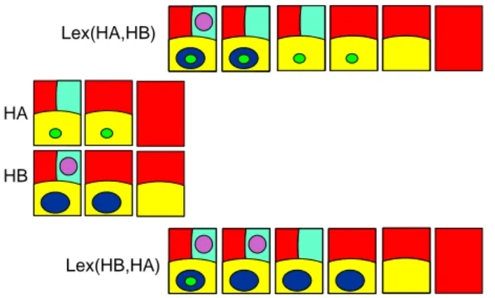
Fig.4 presents too hierarchies HA and HB through their nested partitions. The supremum and in…mum of both hierarchies also are represented. The in…mum takes for each threshold the intersection of the corresponding partitions, ob-tained through intersection of the tiles. The supremum is obob-tained by keeping only the boundaries existing in each component.
Fig.5 presents an initial image to segment.The H component and the V com-ponent of the colour image are segmented separately, yielding two hierarchies. Each hierarchy is illustrated trough one of its thresholds. The in…mum of both
hierarchies combines the features of each of the components, yielding a decent segmentation of the initial image.
Figure 4: Two hierarchies HA and HB and their derived supremum and in…mum
8.3
Lexicographic fusion of strati…ed hierarchies
Let A and B be two strati…ed hierarchies, with their associated distances dA
and dB: In some cases, one of the hierarchies correctly represents the image to segment, but with a too small number of nested partitions. One desires to enrich the current ranking of regions as given by A; by introducing some intermediate levels in the hierarchy. The solution is to combine the hierarchy A with another hierarchy B in a lexicographic order.
One produces the lexicographic hierarchy Lex(A; B) by de…ning its ultra-metric distance ; it is the largest ultraultra-metric distance below the lexicographic distance dA;B classically de…ned by
Initial Image H component V component Infimum Initial Image H component V component Infimum
HA
HB
Lex(HA,HB)
Lex(HB,HA)
Figure 6: Two hierarchies HA and HB and their derived lexicographic combi-nations.
dA;B(C; D) > dA;B(K; L) ,
dA(C; D) > dA(K; L) or
dA(C; D) = dA(K; L) and dB(C; D) > dB(K; L)
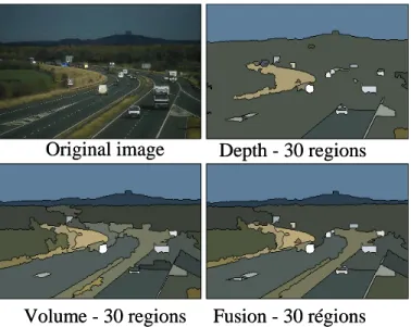
Fig.6 present two hierarchies HA and HB and the derived lexicographic hierarchies Lex(A; B) and Lex(B; A): Fig.7 shows an image which is di¢ cult to segment as it contains small contrasted objects, the cars and the landscape and road which are much larger and less contrasted. Two separate segmenta-tion have been performed. The …rst based on the contrast segments the cars ; the second, based on the "volume" (area of the regions multiplied by the con-trast) segments the landscape. The hierarchy of both these segmentations has been thresholded so as to show 30 regions. The lexicographic fusion of both segmentations Lex(Depth; V olume); also thresholded at 30 regions o¤ers a nice composition of both segmentations.
9
Adjunctions on partial hierarchies
We propose two adjunctions, a …ner and a coarser adjunction on hierarchies or partial hierarchies. The …ner one extends to partial hierarchies the adjunc-tion proposed by J.Serra on partiadjunc-tions [12], extended by Ch. Ronse on partial partitions [7]. The coarser one is presented …rst. It is obtained by taking the supremum and in…mum of PUHDs translated by the translations associated to a structuring element.
Depth - 30 regions
Fusion - 30 régions
Original image
Volume - 30 regions
Depth - 30 regions
Fusion - 30 régions
Original image
Volume - 30 regions
Figure 7: Lexicographic fusion of two hierarchies
9.1
A …rst adjunction based on the supremum and
in…-mum of translated PUHD
9.1.1 De…nition
Given a point O serving as origin, a structuring element B is a family of transla-tionsS n !Ox j x 2 Bo: A set X of P(E) may then be eroded and dilated by this structuring element : the erosion X B = V
x2B
X!
Ox and the dilation X B =
W
x2B
XxO!: As one uses for one operator the vectors Ox and for the other the! vectors Ox =! xO; both operators form an adjunction: for any X; Y 2 P(E);! we have X B < Y , X < Y B:
A hierarchy X 2 X (E) is a collection of sets Xi 2 P(E): Through the
translation by a vector !t ; these sets Xi
!t form a new hierarcy X!t: If is the ultrametric ecart associated to X , the ultrametric ecart associated to X!t will be written !t:
As the partial hierarchies form a complete lattice X (E), we may use the same mechanism for constructing an erosion and a dilation on hierarchies. We de…ne two operators operating on a hierarchy X . For showing that the …rst X B = V
x2BX !
Oxis an erosion and the second X B =
W
x2BX !
xO a dilation, we
9.1.2 Proof of the adjunction
We have to prove that for any two hierarchies X ; Y 2 X (E) : X B < Y , X < Y B:
We will prove the adjunction through the half distance associated to the hierarchies X and Y.
We have the following correspondances between the hierarchies and the ul-trametric ecarts : X $ Y $ Y B = V x2BY ! Ox $ W x2B ! Ox X B = W x2BX ! xO $ z }| {V x2B ! xO X B < Y , X < Y B $ z }| {V x2B ! xO> , > W x2B ! Ox
Let us now prove this last adjunction.
For two arbitrary ultrametric ecarts and : X < Y B , > W
x2B ! Ox , 8x 2 B : > ! Ox, 8x 2 B : xO!> , V x2B ! xO> Remains to establish : V x2B ! xO> , z }| {V x2B ! xO> : z }| {V x2B ! xO> ) V x2B ! xO> since z }| {V x2B !
xOis the largest ultrametric ecart
below V x2B ! xO Suppose now V x2B !
xO> : Since is an ultrametric ecart below
V
x2B ! xO;
it is smaller or equal to the largest ultrametric ecart below V
x2B ! xO; that isz }| {V x2B ! xO
This completes the proof : X < Y B , > W x2B ! Ox , V x2B ! xO> , z }| {V x2B ! xO> , X B < Y
The erosion of a partition by a square structuring element (8 connexity) is illustrated in …g.8, where the smallest squares represent each a pixel.
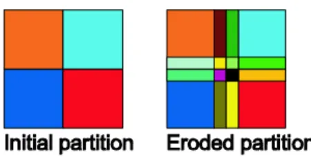
Figure 8: Erosion of a partition by a structuring element equal to the central point and its ’ nearest neighbors. The smallest dots in the right picture show the size of the individual pixels in a square raster. Two neighboring pixels p and q belong to the same region of the eroded partition if there exists a b 2 B such that p + b and q + b both belong to the same tile of the initial partition.
9.1.3 Expression of the erosion and dilation, valid for hierarchies and partial hierarchies
Consider now a partial herarchy X . We have the following correspondances between the hierarchies and the ultrametric ecarts :
X $ X B = V x2BX ! Ox $ W b2B ! Ox X B = W x2BX ! xO $ z }| {V b2B ! xO
The expression of the PUHD is X B(p; q) = W b2B ! Ox (p; q) = W f (p + b; q + b) j b 2 Bg X B(p; q) = z }| {V b2B ! xO (p; q) = z }| { V f (p b; q b) j b 2 Bg
If p B contains an alien x = p + b with a strati…cation level , then (p + b; q + b) and X B(p; q) .
9.1.4 Illustration
We illustrate the erosion and the opening of a one dimensional hierarchy, …rst by a structuring element reduced to two pixels, then by a structuring element made of three pixels. In the …rst case, the erosion and the dilation have to use the structuring element for the erosion and its transposed version for the dilation. Erosion and opening by a pair of 2 pixels.
3 2 1 4 2 3 2 1 4 2 3 2 1 4 2 3 2 1 4 2 3 2 1 4 2 3 2 4 2 1 3 2 4 2 Initial image Right translation Erosion Left translation Opening
Figure 9: Erosion and opening by a pair of pixels: intermediate steps
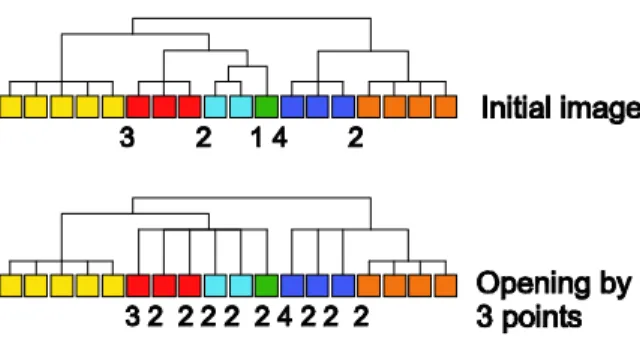
Figure 10: Dendrogram of an initial image and its opening by a segment of 2 points. 3 2 1 4 2 3 2 1 4 2 3 2 1 4 2 3 3 3 2 2 2 4 4 4 2 2 2 3 2 2 2 2 2 4 2 2 2 3 3 3 2 2 2 4 4 4 2 2 2 3 3 3 2 2 2 4 4 4 2 2 2 3 2 1 4 2 Initial image Right translation Left translation Erosion Right translation Left translation Opening Initial image
Figure 12: Dendrogram of an initial image and its opening by a segment of 3 points.
9.2
Adjunction on hierarchies and partial hierarchies,
de-…ned on a tile by tile basis
In this section we recall how J.Serra de…ned an adjunction on partitions and how Ch. Ronse adapted it to partial partitions. We illustrate the method and compare with the adjunction presented previously, based on the supremum and in…mum of translated partitions. We then extend to partial hierarchies the adjunction de…ned by Ch. Ronse for partial partition.
9.2.1 Dilation/erosion on partitions
Description of the algorithm J.Serra proposed in [12] where each tile of the partition is eroded separately. As the resulting collection of sets does not cover the domain E; he completes the empty spaces with singletons.
The adjunct dilation has been de…ned by Ch. Ronse. Il consists in dilating all non singleton sets of a partition, chain all dilated sets with a non empty intersection ; if there are empty spaces, complete with singletons in order to obtain a partition.
Discussion The proposed erosion does not make the distinction between singletons produced by the erosion of some tile of the initial partition and sin-gletons added to …ll empty spaces. For this reason, the adjunct dilation dilates only the non singleton parts of a partition and chains all dilated sets with a non empty intersection. If there are spaces left empty, they are …lled by singletons. An opening and a closing can be classically obtained by chaining the erosion and dilation of the preceding adjunction. The singletons produced by a …rst ero-sion are discarded by the subsequent opening. Like that, a tile which is identical with the structuring element is pulverized into singletons by the opening.
It is to note that the singletons form a role apart from any other set, as the chaining between sets with non empty intersection can never pass through singletons : the intersection of a set and a singleton is always reduced to the singleton itself.
9.2.2 Adjunction on partial partitions
Description of the algorithm Using partial partitions alleviates this dif-…culty as shown by Ch. Ronse. The erosion of a partial partition consists in eroding each tile of the partial partition separately, producing a new partial partition, whose support contains all eroded sets produced, including the single-tons. Therefore there is no need to complete the empty spaces with singletons, as the support of the partial partitions varies.
The dilation consists in dilating all tiles of the partial partition (including the singletons) and chain all dilated sets with a non empty intersection. The support of the initial partition may like that also be dilated, in order to contain all sets produced by the dilation. Here again, there is no need to …ll empty spaces with singletons.
Discussion Here, there is no need of …lling singletons, as the support of the partial partition is variable. If after an erosion, there exist singletons in the resulting partial partitions, they duly correspond to eroded sets of the initial partial partition. Therefore they may be dilated to obtain the openings. 9.2.3 Adjunctions on hierarchies and partial hierarchies
In this section, we establish the PUHD (partial ultrametric half distance) for Ronse’s adjunction for partial partitions. It happens that the obtained expres-sion is also valid for hierarchies and partial hierarchies.
Let be the PUHD (partial ultrametric half distance) representing a partial hierarchy and (" ; ) the adjunction of the PUHDs.
Adjunctions on partitions and partial partitions
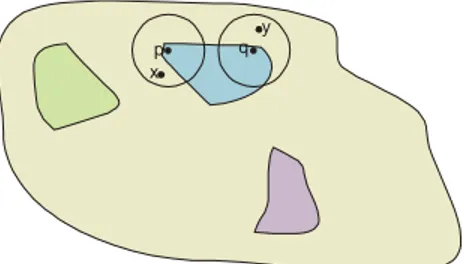
Erosion We illustrate the method with a partition, as illustrated in …g.13. The points p and q belong to the same tile of the partition eroded by a structur-ing element B, if they are centers of disks entirely included in the same tile of the initial partition. In such a case all pairs x; y 2 Bp[ Bq belong to the same tile of
the partition, hence (x; y) = 0: For the pair p; q we have " (p; q) = 0: Inversely if these conditions are not veri…ed, there exists a pair of pixels x; y 2 Bp[ Bq
which does not belong to the same tile of the partition and (x; y) = 1: It follows from this analysis, that the PUHD " of the eroded hierarchy can be expressed as
" (p; q) =Wf (x; y) j x; y 2 Bp[ Bqg
Consider now a point p such that Bp is not included in any tile of the
partition . If s 2 Bp; there exists then a t 2 Bp such that (s; t) = 1;
otherwise Bp would belong to the same tile of the partition. For such a point