Statistical Modeling of the Patches DC Component for Low-Frequency Noise Reduction

HAL Id: hal-02024205

https://hal.archives-ouvertes.fr/hal-02024205v2

Submitted on 22 Feb 2019

HAL is a multi-disciplinary open access

archive for the deposit and dissemination of

sci-entific research documents, whether they are

pub-lished or not. The documents may come from

teaching and research institutions in France or

L’archive ouverte pluridisciplinaire HAL, est

destinée au dépôt et à la diffusion de documents

scientifiques de niveau recherche, publiés ou non,

émanant des établissements d’enseignement et de

recherche français ou étrangers, des laboratoires

Statistical Modeling of the Patches DC Component for

Low-Frequency Noise Reduction

Antoine Houdard

To cite this version:

Antoine Houdard. Statistical Modeling of the Patches DC Component for Low-Frequency Noise

Reduction. 2019 27th European Signal Processing Conference (EUSIPCO), Sep 2019, La Corogne,

Spain. �10.23919/EUSIPCO.2019.8903131�. �hal-02024205v2�

Statistical Modeling of the Patches DC

Component for Low-Frequency Noise Reduction

Antoine Houdard

MAP5, Universit´

e Paris Descartes

houdard.wp.imt.fr

Abstract

This work is devoted to patch-based image denoising. Assuming an additive white Gaussian noise (AWGN) on patches, we derive correspond-ing models on centered patches and on their DC components. Then we propose to treat the two components separately. Finally, we provide ex-periments with the recent denoising method HDMI [1] and we show that our approach improves the denoising quality, particularly for residual low frequency noise.

1

Introduction

Context In this paper, we focus on image denoising, which aims to estimate an image_pu from its noisy observation

v “ u ` e P Rn, (1)

where e „ N p0, σ2Inq is an additive white Gaussian noise (AWGN) and u the

underlying clean image. Some of the recent denoising methods are based on a statistical modeling of the image patches [2, 3, 4, 5, 1]. For each patch i P t1, . . . , nu seen as vector of size p “ s ˆ s, model (1) yields

Yi“ xi` Ni, (2)

where YiP Rp is the observed random vector modeling the i-th patch, xiP Rp

is the underlying clean patch and Ni „ N p0, σ2Ipq is a Gaussian white noise.

The idea is then to set a prior model on the clean patch xi seen as a realization

of a random vector Xi. The model therefore rewrites

Yi“ Xi` Ni, (3)

and Bayes’ theorem yields the posterior Xi|Yi. Finally, each clean patch can be

Convenient priors for computing this estimator (4) are Gaussian priors [2] or Gaussian mixture models (GMM) [3, 5, 1]. The use of these priors has been widely studied and it appears that the covariance matrix of these models can encode local structures up to some contrast change [6]. This permits to regroup more patches under the same Gaussian model and then allows for a better estimate of its parameters. There is however a drawback: grouping patches in this way makes the mean of the model less informative. This yields an estimate for each patch that has some bias. This produces the low frequency residual noise that appears in the result of model-based patch-based denoising methods. Figure1 (b) illustrates this phenomenon in the case of the HDMI method [1], with strong noise and small patches. A large part of this low frequency noise seems to come from a poor estimation of the mean of each patch. Indeed, the image (d) from figure1made up of the mean of each patch of the noisy image (a) has the same patterns than the image (c) which is made up of the mean of each patch of the denoised image (b). Moreover, replacing the mean of each denoised patches from (b) with the true mean of the oracle (f), yields a denoised image (c) that is way better, both in terms of Peak Signal to Noise Ratio (PSNR) and visual quality, than the image (b). In addition, some methods from the literature [5, 4] also seem to suggest that removing the mean – also called the DC component – of the patches may improve the denoising quality.

Proposed work In this work, we propose to study the decomposition of the patches into the DC component and the centered component for denoising pur-poses. To do so, we define the centered observed random variable Y_ic“ Yi´ sYi1p,

where s Yi“ 1 p p ÿ j“1 Yipjq, (5)

is the mean of Yi and 1p“ p1, . . . , 1q P Rp. The model (3) can then be divided

into the two following problems s

Yi “ sXi` sNiP R, (6)

and

Y_ic“ X_ic` N_icP Rp. (7) We propose to model the noise components Nc

i (section 2) and sNi (section3)

of these two problems. Then we suggest in section4 various solutions that can enhance the denoising results of the patch-based denoising method HDMI [1], and we provide numerical experiments for these solutions.

2

Modeling the centered noise

The centered noise is defined by Nc

i “ Ni´ ĎNi1pand then the j-th entry of Nic

is Nicpjq “ Nipjq ´ 1 p p ÿ k“1 Nipkq, (8)

(a) (b) (c)

(d) (e) (f)

Figure 1: (a) noisy image (standard deviation 30{255). (b) image denoised with HDMI [1] (patches 7 ˆ 7), PSNR = 31.92 dB. (c) image from the denoised patches of (b) with DC component corrected with oracle value (f), PSNR = 33.78 dB. (d) DC component of the patches of (a). (e) DC component of the patches of (b). (f ) DC component of the oracle image (ground truth).

since Ni is a Gaussian random vector, Nic is also Gaussian. Then, we can

compute its mean and its covariance matrix coordinate by coordinate. That gives for the mean

E rNicpjqs “ E rNipjqs ´ 1 p p ÿ k“1 E rNjpkqs “ 0. (9)

E rNicpkqN c iplqs “ E rNipkqNiplqs ´1 p p ÿ m“1 E rNipmq pNicplq ` N c ipkqqs ` 1 p2 p ÿ m“1 p ÿ n“1 E rNipmqNicpnqs “ σ2 ˆ δkl´ 2 p` p p2 ˙ “ σ2 ˆ δkl´ 1 p ˙ . Finally, we have Nc i „ N p0, ΣNc iq with ΣNc i “ σ2 p ¨ ˚ ˚ ˚ ˚ ˝ p ´ 1 ´1 ¨ ¨ ¨ ´1 ´1 p ´ 1 ... .. . . .. ´1 ´1 ¨ ¨ ¨ ´1 p ´ 1 ˛ ‹ ‹ ‹ ‹ ‚ . (10) Since ΣNc

i is a real symmetric matrix, there exists an orthonormal basis that

diagonalizes it. Given that its eigenvalues are p (of multiplicity p ´ 1) and 0, we can build an orthogonal matrix Q such that

ΣNc i “ Q ˆ σ2_I p´1 0 0 0 ˙ QT. (11)

It is worth noticing that the unit eigenvector corresponding to the eigenvalue 0 is?1

pp1, . . . , 1q. The change of basis Q

T _{applied to the centered noise then yields}

QT_Nc

i „ N p0, diagpσ2Ip´1, 0qq. Finally, centering the noise implies a dimension

reduction. The total variance of the centered noise defined as TVarpNicq “ Er}N c i} 2 2s (12) “ TrpΣNc iq “ pp ´ 1qσ 2 ₍₁₃₎ “p ´ 1 p TVarpNiq (14)

is also reduced by a factor pp ´ 1q{p.

3

Modeling of the DC component

Since the initial noise model on a patch Ni is a Gaussian vector, its mean is a

Gaussian random variable sNi „ N p0,σ

2

pq. Then, reshaping problem (6) as an

image yields the new image denoising problem with additive Gaussian noise s

where sY , sX and sN are the images of Rn whose values at pixel i are sYi, sXi and

s

Ni. The major difference is that the noise is now colored. Indeed, if we consider

two random variables sNi and sNj within a same area of s ˆ s pixels, they are

issued from two overlapping patches and thus are not independent.

However, we can still perform patch-based image denoising on this problem: let us consider patches of the same size p “ s ˆ s from this new image. We define the patches Zi “ πip sY q, Wi “ πip sXq and Mi “ πip sN q, where πi is the

i-th patch extraction operator. We consider the patch noise model

Zi“ Wi` Mi, (16)

with Mi modeling the noise. Since Mi “ p sNi1, . . . sNipq, all its entries are linear

combinations of the noise components of the problem (1) that are i.i.d following N p0, σ2

q. Therefore, all linear combinations of entries of Mi are also Gaussian.

This shows that Mi is a Gaussian vector. We can now compute its mean and

covariance matrix.

The mean of Miis obviously 0pthe coefficients of the covariance matrix ΣMi

are given by pΣMiqkl“ E “ s Nik, sNil ‰ “ σ 2 p2Ckl, (17)

where Ckl is the number of common pixels between the two patches of the

original image from which sNik and sNil are derived. This yields after counting

ΣMi “ σ2 p2B b B (18) where B “ ¨ ˚ ˚ ˚ ˚ ˝ s ps ´ 1q ¨ ¨ ¨ 1 ps ´ 1q s . .. ... .. . . .. . .. ps ´ 1q 1 ¨ ¨ ¨ ps ´ 1q s ˛ ‹ ‹ ‹ ‹ ‚ , (19)

and b is the Kronecker product. In order to use a denoising method that has been designed for AWGN, we want to perform a change of basis for the data. To do so, we study the structure of ΣMi. First, we show that B is symmetric

positive-definite. Using the Sylvester’s criterion, it is sufficient to show that all of the leading principal minors of B are positive. These minors of size d P t1, . . . , su are given by md “ ˇ ˇ ˇ ˇ ˇ ˇ ˇ ˇ ˇ ˇ s ps ´ 1q ¨ ¨ ¨ ps ´ d ` 1q ps ´ 1q s . .. ... .. . . .. . .. ps ´ 1q ps ´ d ` 1q ¨ ¨ ¨ ps ´ 1q s ˇ ˇ ˇ ˇ ˇ ˇ ˇ ˇ ˇ ˇ , (20)

Adding the first column in the last one yields md“ p2s ´ d ` 1q ˇ ˇ ˇ ˇ ˇ ˇ ˇ ˇ ˇ ˇ s ps ´ 1q ¨ ¨ ¨ 1 ps ´ 1q s . .. ... .. . . .. . .. 1 ps ´ d ` 1q ¨ ¨ ¨ ps ´ 1q 1 ˇ ˇ ˇ ˇ ˇ ˇ ˇ ˇ ˇ ˇ , (21)

then subtracting the second and the last column to the first one gives

md“ p2s ´ d ` 1q ˇ ˇ ˇ ˇ ˇ ˇ ˇ ˇ ˇ ˇ 2 ps ´ 1q ¨ ¨ ¨ 1 0 s . .. ... .. . . .. . .. 1 0 ¨ ¨ ¨ ps ´ 1q 1 ˇ ˇ ˇ ˇ ˇ ˇ ˇ ˇ ˇ ˇ , (22)

Finally, developing the determinant with respect to the first column and repeat-ing the two last steps yields

md“ p2s ´ d ` 1q2d´2 ą 0. (23)

This shows that B is a positive-definite matrix. Then B b B is also symmetric positive-definite as the Kronecker product of two positive-definite matrices and the Cholesky decomposition yields an invertible matrix L such that B b B “ LLT_{. Therefore, the problem}

L´1_Z

i“ L´1Wi` L´1Mi, (24)

is an AWGN problem with noise variance σ2{p2Ip and a denoising method such

as HDMI can be used to find an estimate {L´1_W

i that gives an estimate of Wi

by xWi“ L {L´1Wi.

4

Experiments

In this section, we take advantage of the previous modeling in order to propose various strategies for improving the denoising result of model-based patch-based denoising methods. For this testing part, we propose to use the HDMI method [1] which has the advantage of using only statistical tools. The principle of this method is rather simple:

1. It uses a GMM with intrinsic lower dimensions to model clean patches; 2. This model is inferred on the noisy patches with an expectation–maximization

(EM) algorithm;

3. The clean patches are estimated with the conditional expectation (4), which has a closed-form and is numerically stable (proposition 1 of [1]).

4.1

Denoising the DC component

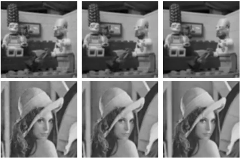
In section3, we have proposed to reshape the DC component of all patches into an image and to extract patches of this image in order to perform patch-based denoising on it. We showed that the noise model on these patches is an AWGN in a given basis L. We can therefore apply the HDMI method directly on (24). Figure 2 shows the result of the denoising of the DC images from the images simpson and lena with a noise of standard deviation σ “ 30{255. Note that the results are quite good since the problem (24) is an easier problem than the original one (3). Indeed, the dynamic of the DC image is quite the same as the one of the original image whereas the dynamic of the noise is reduced by a factor p. Therefore, the signal-to-noise ratio of the problem (16) is about p times larger than the one of the original problem (3). Finally, with this step, we obtain for each patch i an accurate estimate xXĎi of its DC component.

Figure 2: Left: noisy DC image. Middle: denoised DC image (’simpson’ PSNR = 40.64 dB , ’lena’ PSNR = 40.89 dB). Right: oracle DC image. Top line is the from the simpson image and bottom line from the lena image both with noise of standard deviation σ “ 30{255.

4.2

Denoising the patches

In order to perform the final patch denoising, we expose hereafter two strategies. For each of these strategies, we propose numerical examples and we discuss the improvements they bring for the denoising task.

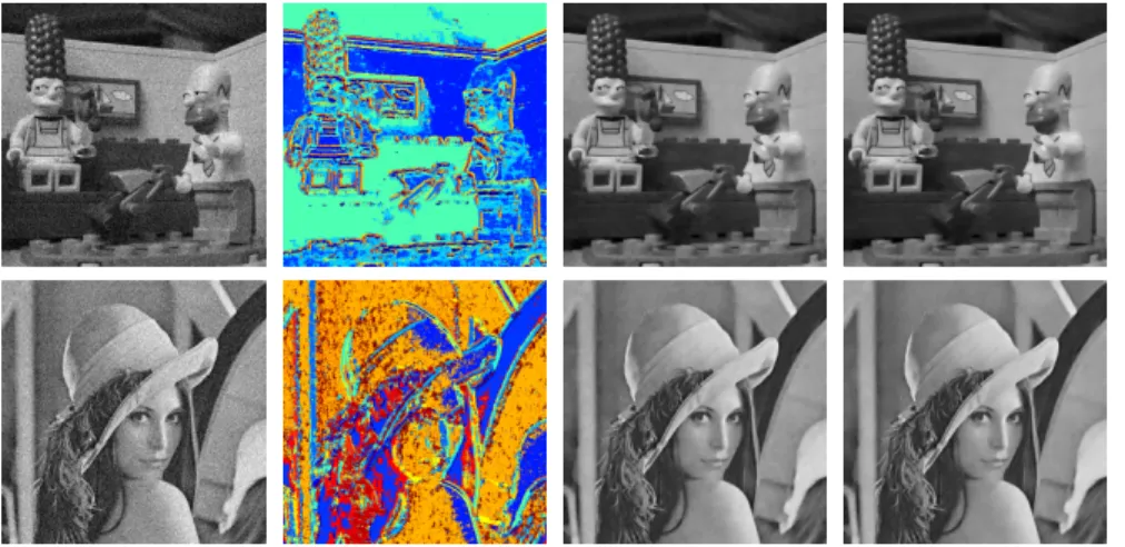
Figure 3: From left to right. Noisy images (standard deviation 30{255). HDMI resulting groups. Images denoised by HDMI (lena 31.09dB, simpson 32.46dB). Images denoised with method4.2.1(lena 31.19dB, simpson 32.58dB).

4.2.1 Correction of the DC component afterwards

The first idea is to run the HDMI method on the original patches yi, yielding

for each patch i an estimate xXi, and then to correct this estimate with the

estimated DC component xXĎi. That is, to consider the final estimate

Est1pXiq “ xXi´XĎx_i1_p` xXĎ_i1_p. (25) This strategy improves the denoising quality compared to the original denoising, as illustrated in Figure 3. The low frequency noise is visually reduced and in term of PSNR, the results show an improvement of « 0.1dB for both images. However, this does not use the modeling of the centered noise from section 2, and the grouping of the patches from the HDMI model remains the same. 4.2.2 Learn a model on the centered patches

The second strategy is to learn the model on the centered patches Xc _{in order}

to group together patches with various contrasts. To do so, we can apply the change of basis QT from section2 on the problem (7). This yields

QTY_ic“ QTX_ic` QTN_ic, (26) with the last line of this equality being ĎYc

i “ ĎXic which is always true since

Ď Yc

i “ ĎXic“ 0 by definition. Removing this last dimension then yields an AWGN

problem in dimension p´1 that can be denoised with the HDMI algorithm. This gives us an estimate of the centered patch xXc

i and therefore the final estimate

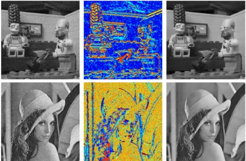
Figure 4: From left to right. Noisy images (standard deviation 30{255). Re-sulting groups of method 4.2.2. Denoising with method 4.2.2 (lena 31.14dB, simpson 32.58dB).

Figure4shows the result of this strategy. The advantage of learning the model on the centered patches is that the patches with same structure but different contrasts are grouped together (figure 4). This can make the estimate of the covariance matrix easier. However, this centered problem has a lower signal-to-noise ratio than the original problem since the centering of the patches has reduced the dynamic. Therefore, the algorithm is more likely to missclassify some fine textures. This strategy still leads to a visual and PSNR improvement but seems not to be better than the previous solution.

4.3

Discussion

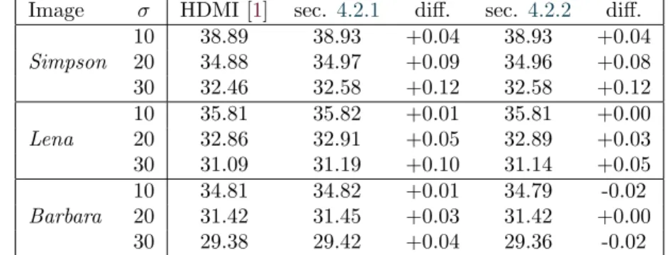
Finally, we propose in table1the results of the two presented strategies for the three images simpson, lena and barbara with different level of noise. This shows that the first strategy always improve the denoising quality, with a larger im-provement for images that have less textures like simpson. The second strategy seems also to work well in this precise case but fail to improve the result in the case of barbara which has a lot of fine texture. The other trend that appears is the better improvement for high variance noise than for low variance noise. This is due to the use of the same patch size for all experiments. Indeed, for a given patch size, the residual low frequency noise increases with the variance of the initial noise.

Table 1: Results in PSNR (dB) of the enhancement methods from sec-tion 4.2.1 and 4.2.2 for the images simpson, lena and barbara with different noise levels.

Image σ HDMI [1] sec. 4.2.1 diff. sec. 4.2.2 diff. Simpson 10 38.89 38.93 +0.04 38.93 +0.04 20 34.88 34.97 +0.09 34.96 +0.08 30 32.46 32.58 +0.12 32.58 +0.12 Lena 10 35.81 35.82 +0.01 35.81 +0.00 20 32.86 32.91 +0.05 32.89 +0.03 30 31.09 31.19 +0.10 31.14 +0.05 Barbara 10 34.81 34.82 +0.01 34.79 -0.02 20 31.42 31.45 +0.03 31.42 +0.00 30 29.38 29.42 +0.04 29.36 -0.02

5

Conclusion

In this work, we have studied the effect of patch centering for model-based patch-based denoising methods. For this purpose, we have proposed a modeling of the centered noisy patches and a modeling of the DC component of the noise. These modeling have led us to strategies for improving the result of existing denoising methods, especially to reduce low-frequency residual noise. The results obtained with the HDMI method on grayscale images show improvements, both visually and in term of PSNR.

In future work, we would like to study the links between this approach and multiscale frameworks. Then, in a second step, we would like to propose a discussion on the strategy to be adopted for color images.

References

[1] Antoine Houdard, Charles Bouveyron, and Julie Delon, “High-dimensional mixture models for unsupervised image denoising (hdmi),” SIAM Journal on Imaging Sciences, vol. 11, no. 4, pp. 2815–2846, 2018.

[2] M. Lebrun, A. Buades, and J. M. Morel, “A Nonlocal Bayesian Image Denoising Algorithm,” SIAM J. Imaging Sci., vol. 6, no. 3, pp. 1665–1688, Sept. 2013.

[3] Yi-Qing Wang and Jean-Michel Morel, “SURE Guided Gaussian Mixture Image Denoising,” SIAM J. Imaging Sci., vol. 6, no. 2, pp. 999–1034, May 2013.

[4] Daniel Zoran and Yair Weiss, “From learning models of natural image patches to whole image restoration,” in 2011 Int. Conf. Comput. Vis. Nov. 2011, pp. 479–486, IEEE.

[5] Afonso M Teodoro, Mariana SC Almeida, and M´ario AT Figueiredo, “Single-frame image denoising and inpainting using gaussian mixtures.,” in ICPRAM (2), 2015, pp. 283–288.

[6] Julie Delon and Antoine Houdard, Gaussian Priors for Image Denoising, chapter , pp. 125–149, Springer International Publishing, Cham, 2018.