A Benchmark of Four Methods for Generating 360° Saliency Maps from Eye Tracking Data

HAL Id: hal-01953877

https://hal.inria.fr/hal-01953877

Submitted on 13 Dec 2018

HAL is a multi-disciplinary open access

archive for the deposit and dissemination of

sci-entific research documents, whether they are

pub-lished or not. The documents may come from

teaching and research institutions in France or

abroad, or from public or private research centers.

L’archive ouverte pluridisciplinaire HAL, est

destinée au dépôt et à la diffusion de documents

scientifiques de niveau recherche, publiés ou non,

émanant des établissements d’enseignement et de

recherche français ou étrangers, des laboratoires

publics ou privés.

A Benchmark of Four Methods for Generating 360°

Saliency Maps from Eye Tracking Data

Brendan John, Pallavi Raiturkar, Olivier Le Meur, Eakta Jain

To cite this version:

Brendan John, Pallavi Raiturkar, Olivier Le Meur, Eakta Jain. A Benchmark of Four Methods for

Generating 360° Saliency Maps from Eye Tracking Data. Proceedings of The First IEEE International

Conference on Artificial Intelligence and Virtual Reality, Dec 2018, Taichung, Taiwan. �hal-01953877�

A Benchmark of Four Methods for Generating

360

◦

Saliency Maps from Eye Tracking Data

Brendan John

, Pallavi Raiturkar

, Olivier Le Meur

, Eakta Jain

∗_{University of Florida, Gainesville, US} †_{Univ Rennes, CNRS, IRISA, France}

Abstract—Modeling and visualization of user attention in Vir-tual Reality is important for many applications, such as gaze pre-diction, robotics, retargeting, video compression, and rendering. Several methods have been proposed to model eye tracking data as saliency maps. We benchmark the performance of four such methods for 360◦ images. We provide a comprehensive analysis and implementations of these methods to assist researchers and practitioners. Finally, we make recommendations based on our benchmark analyses and the ease of implementation.

Index Terms—Saliency, Visualization, Eye movements in VR, 360 images

I. INTRODUCTION

With the explosive growth of commercial VR and AR sys-tems, there is increased access to innovative 3D experiences. In particular, 360◦ images and videos are being used for entertainment, storytelling, and advertising. Content creators are actively working out techniques and building tools to guide user attention in these new media. A critical enabler for these efforts is measuring and visualizing eye tracking data. Eye trackers built into VR headsets serve as a reliable tool to understand how attention is allocated in 3D environments.

The study of attention and eye movements in 2D content is well established. Saliency maps highlight regions that attract the most visual attention and have applications in predicting gaze [1], compression [2], and selective rendering [3] to name a few. In 360◦ images, the user is surrounded by a photo-realistic virtual scene. Because only a fraction of the scene is viewed at once, the allocation of visual attention is different than 2D content. Moreover, due to the spherical nature of 360◦ content, novel saliency map generation methods are required. To generate 2D saliency maps, eye tracking data is pro-cessed to identify fixations. Fixations are aggregated in a map that is convolved with a 2D Gaussian kernel. For 2D displays the number of pixels per visual degree is assumed to be the same in horizontal and vertical directions, so an isotropic Gaussian is used. The Kent distribution is an analog to a 2D Gaussian on the surface of a 3D sphere [4]. 360◦ images encode spherical data, and the natural extension is to process them using such a distribution. However, computing a Kent based saliency map is slow due to a spatially varying kernel. Fortunately, several approximate alternatives exist.

In this paper, we benchmark four alternative methods for generating 360◦ saliency maps. We report accuracy and run-time for each algorithm, and present pseudocode to implement them. Based on these analyses and ease of implementation, we identify the most favorable approach.

II. BACKGROUND

Saliency maps aggregate data from multiple observers into a representative map of human attention. Typically, saliency maps are generated by summing fixations from each observer into a discrete fixation map,

Fi(x) =

M

X

k=1

δ(x − xi_k), (1)

where M is the number of fixations by the ith observer, x represents two dimensional pixel coordinates in the image, and xi

k represents the coordinates of the k

th_{fixation [5]. δ is the}

Dirac function, which evaluates to 1 at δ(1), and 0 everywhere else. All maps from N observers are averaged to produce a unique representative map,

F (x) = 1 N N X i=1 Fi(x) (2)

This fixation map is convolved with a 2D Gaussian kernel to produce a continuous map highlighting salient regions instead of individual pixels. The Gaussian kernel accounts for noise in measurement, such as calibration error, as well as falloff in visual acuity outside the foveal region. The standard deviation parameter, σ, is typically set between 1◦ and 5◦ visual angle due to the size of the foveal region and eye tracker error [6]. For 360◦ content, saliency researchers need to translate existing 2D methodologies to immersive 3D environments. 2D metrics are well understood [5], but they must be reconsidered for 360◦ saliency maps and scanpaths. As saliency prediction models adapt to 360◦[7]–[10], there is a need for a standard-ized method to evaluate them against ground truth. Several eyetracking datasets are available for 360◦ images and video, with their own method for generating saliency maps [11]–[13].

III. METHODSTOGENERATESALIENCYMAPS IN360◦ Four methods of generating 360◦ saliency maps have been proposed recently: applying a Gaussian kernel to fixations on the viewport and projecting the resulting maps onto the surface of the viewing sphere [12], applying a Gaussian kernel to the face of a cubemap [9], modifying the Gaussian kernel based on row [14], and simply applying an isotropic Gaussian kernel on the equirectangular image [11]. These methods have been proposed in separate publications, with algorithmic details scattered between supplementary materials, or as part of datasets. Here, we collect these alternatives in one place,

clarify algorithmic details, and benchmark their performance using a Kent distribution based method as ground truth. We briefly summarize and present pseudocode for the Kent based method, and the four approximate methods. For each method the output is a saliency map, S, that is then normalized such that all of the values sum to one. A square kernel is used for ease of implementation, with kernel size set to 12 times the number of pixels per degree rounded up to an odd number. This size is larger than usual to ensure that all non-zero values are included. Helper functions are defined in the Appendix.

Kent Distribution: The Kent distribution is an isotropic bivariate normal distribution defined on the surface of a three dimensional unit sphere [4]. While the complete 5 parameter distribution is anisotropic, we use the simplified isotropic form. The probability density function f is defined as

f (~x, κ, ~γ) = κe

κ~γ·~x

4πsinh(κ), (3) where ~_{x ∈ R}3 _{is an input vector representing a point on the}

sphere. The parameter κ > 0 represents the concentration of the probability density function. The parameter ~_{γ ∈ R}3 _is

the mean direction of the distribution, around which points are normally distributed. Pixels in the equirectangular image x, y map to azimuth and elevation angles θ, φ. These angles are converted from spherical coordinates to a 3D vector in cartesian coordinates ~x. We compute the kernel weights by inputting the pixel neighborhood N (x, y, kernel size) as vec-tors into f , where ~γ is a vector that represents the current pixel. Due to unequal sampling of the sphere in equirectangular images, the kernel must be recomputed for each row. Input to this method is a fixation map F , and parameter κ.

1: procedure KENT(F ,κ)

2: S ← zeros(num rows, num cols)

3: for r = 1 to num rows do . Parallelizable loop 4: φ ← π|r/num rows − 0.5|

5: θ ← 0 . θ is constant

6: c = num cols/2 . c is constant 7: ~γ ← sph2cart(θ, φ, 1)

8: K ← f (N (c, r, kernel size), κ, ~γ)

9: N ormalize K . Kernel weights sum to 1 10: Srow← F ~ K . Optimized to only output row r

11: S(r) = Srow

In a MATLAB implementation we found that using a κ value of 707 or higher produces a result too large to fit in a 64 bit floating point number. Typical values of κ will be larger than this for modeling 1◦ or less of visual angle in saliency map generation. HPF1 for high precision floating point numbers is needed, which increases the amount of time needed to perform the operations invoked by f . The following methods either approximate the Kent distribution (modified Gaussian), or operate outside the spherical domain.

Isotropic Gaussian Method: For 2D map generation a spa-tially invariant kernel is used, filtering the image in seconds.

1

https://www.mathworks.com/matlabcentral/fileexchange/36534-hpf-a-big-decimal-class

While quick, this computation does not account for distortions in the equirectangular image. Input to this method are a fixation map F , and standard deviation σ.

1: procedure ISOTROPIC(F,σ)

2: Gσ← 1d gaussian(σ, kernel size)

3: K ← Gσ· GTσ

4: _{S ← F ~ K . ~ indicates 2D convolution} Modified Gaussian Method: Upenik & Ebrahimi [14] intro-duce a modified Gaussian kernel that accounts for equirect-angular distortions near the poles. A scale factor of _cosφ1 is computed for each elevation angle φ, to stretch an isotropic Gaussian kernel horizontally. A bivariate Gaussian kernel is computed for each row as the matrix product

K = Gσy · G

T

σx, (4)

where Gσy is a column vector representing a 1D Gaussian

with standard deviation σy in pixels, and GTσx is a row vector

representing a 1D Gaussian where σx = _cosφσy . This method

applies a different filter at each row, requiring many 2D convolutions. This method has a similar runtime and structure to the Kent distribution, but is much easier to implement.

1: procedure MODIFIEDGAUSSIAN(F ,σ) 2: S ← zeros(num rows, num cols)

3: for r = 1 to num rows do . Parallelizable loop 4: φ ← π|r/num rows − 0.5|

5: Gσy ← 1d gaussian(σ, kernel size)

6: Gσx← 1d gaussian(σ/cosφ, kernel size)

7: K ← Gσy· G

T σx

8: Srow ← F ~ K . Optimized to only output row r

9: S(r) = Srow

Cubemap Method: Cubemaps reduce image distortions by projecting the spherical image onto cube faces representing perspective views from within the sphere. This format al-lows each face to be filtered with an isotropic Gaussian, but introduces discontinuities at the borders. To reduce this effect, cubes at two orientations are aligned and combined in equirectangular format to generate one representative map for the image. Weights W1and W2 are applied with an

element-wise multiplication to reduce the contribution of pixels near the edges of each face, as described by [9]. Transforming high resolution images between formats is time consuming, and the method does not completely remove border discontinuities.

1: procedure CUBEMAP(F ,σ)

2: Frot ← rotatesphereXY Z(F,pi₄, 0,pi₄)

3: Gσ← 1d gaussian(σ, kernel size)

4: K ← Gσ· GTσ

5: Cube1← equirect2cube(F ) ~ K

6: Cube2← equirect2cube(Frot) ~ K

7: S1← cube2equirect(Cube1)

8: S2← cube2equirect(Cube2)

9: S ← W1. ∗ S1+ W2. ∗ S2

Viewport Method: 360◦ content is realized as a projection of the spherical image onto a viewport determined by the observer’s head orientation. A Gaussian kernel can then be

applied directly within the viewport, and projected back onto the equirectangular image [12]. These values are summed across the equirectangular saliency map for each fixation. This method’s runtime scales with the number of fixations. It can produce projection errors due to interpolation. The process of projecting each viewport onto the image generally has the longest runtime with high resolution images, and requires the HMD’s horizontal and vertical field of view, f ovx and f ovy.

Input for this method is a list of fixations in HMD screen space, head rotation, and the horizontal and vertical standard deviations of the 2D Gaussian in pixels, σx and σy.

1: procedure VIEWPORT(FIXATIONS,ROTATIONS,σx,σy)

2: S ← zeros(num rows, num cols) 3: for i = 1 to M f ixations do

4: viewport ← zeros(viewport size) 5: x, y ← f ixationi

6: R ← rotationi

7: viewport(y, x) = 1

8: Gσy ← 1d gaussian(σy, kernel size)

9: Gσx ← 1d gaussian(σx, kernel size)

10: K ← Gσy · Gσx

11: Sviewport← viewport ~ K

12: Sequirect← vp2sphere(Sviewport, R, f ovx, f ovy)

13: S += Sequirect

IV. BENCHMARKMETHODOLOGY& RESULTS We benchmark the isotropic Gaussian, Viewport, Cubemap, and modified Gaussian saliency map methods to evaluate accuracy and performance. The Kent based method serves as ground truth, taking hours to compute for each image at full resolution. The modified Gaussian method also has a long runtime as it performs a convolution at each row. Instead, we first reduce the resolution of the image to 5% it’s original size using MATLAB’s imresize, then apply the modified Gaussian method. The result is then returned to the original resolution using bicubic interpolation. 5% scale was selected to generate a map in several seconds, with less than 2% deviation from the full resolution output. While saliency map generation is typically an offline process, our goal is to select a method that is efficient to ease analysis for researchers, and for real time applications such as 360◦ video streaming to many clients.

We use publicly available data and metrics for evaluation [12]. The dataset contains 40 images, each with fixations from at least 40 different observers classified using velocity thresholding. The image resolution ranged from 5376x2688 to 18332x9166. For our benchmark the saliency maps for each method are compared with the Kent based maps, and results are averaged across all images. Head orientation data was not provided with the dataset, meaning we had to use the provided maps instead of generating our own for the Viewport method. The parameter σ=3.34◦ was used for each method to match the dataset. The parameter κ=430 was found to match σ=3.34◦ by comparing the mean and standard deviation of points generated on a sphere using the Kent distribution, and points from a projected 2D Gaussian. We have not yet derived a closed form relation between the two parameters. Results were

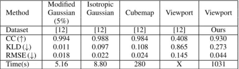
Method

Modified Isotropic

Cubemap Viewport Viewport Gaussian Gaussian (5%) Dataset [12] [12] [12] [12] Ours CC (↑) 0.994 0.988 0.984 0.408 0.930 KLD (↓) 0.011 0.097 0.108 0.865 0.273 RMSE (↓) 0.018 0.022 0.024 0.145 0.044 Time(s) 5.16 8.80 280 X 1031 TABLE I: Computed metrics for each method compared with ground truth Kent saliency maps. We implemented the Viewport method for use with our own dataset.

generated on a PC with an 8 core AMD FX-8350 processor, and MATLAB R2017a. MATLAB routines for these methods have been made publicly available, including a parallelized implementation of the Kent and Modified Gaussian method. The serialized code was used for the benchmark.

The saliency map metrics Correlation Coefficient (CC), KL Divergence (KLD), and RMSE were used to measure similarity between each of these maps and the Kent method map for all images [5]. CC ranges from 0 to 1, with high values indicating better performance. KLD represents divergence between two probability distributions, meaning lower values are considered a good score. Similarly, a low RMSE indicates a better approximation. Table I shows the computed metrics averaged across each image in the dataset. The modified Gaussian at 5% scale has the highest CC value, lowest KLD, and lowest RMSE indicating it had the highest similarity to the Kent saliency maps. In addition to high accuracy, the modified Gaussian at 5% is also efficient with an average runtime of 5.16 seconds. The Viewport method maps provided with the dataset have no runtime, as they were read from file. We found that these maps scored lowest of all evaluated methods. An explanation for this could be that an isotropic Gaussian was used within the viewport when generating saliency maps. The viewport size is based on the Oculus DK2 screen and field of view, which is 1920x1080 and 94◦x105◦, meaning the number of pixels per degree is different in horizontal and vertical directions. To avoid this limitation, we use pixels per degree in the horizontal and vertical directions and apply an anisotropic Gaussian.

To evaluate the effect of an anisotropic Gaussian kernel, we implemented the Viewport method to process our own data. We conducted an IRB approved experiment on 22 participants with a similar protocol to [12], using the same VR eye tracking equipment and images. We computed Kent and Viewport saliency maps for each image and evaluate them in the same manner, shown in Table I. We produced more accurate results, raising CC scores from 0.41 to 0.93, and reducing RMSE from 0.15 to 0.04 across the same images. This effect can be observed visually, as Figure 1 compares heat maps from both Viewport and Kent method outputs.

V. DISCUSSION

We found that a subsampled version of the modified Gaus-sian method is sufficient for generating accurate 360◦saliency maps efficiently. While a sub-sampled Kent method could also be used, the parameter κ is not as intuitive as σ, which

Fig. 1: Cropped region of Kent and Viewport saliency heat maps provided with [12] and computed from our own data collection. Red indicates large saliency values, and blue indi-cates low values. Our implementation of the Viewport method better overlaps with the Kent output as it does not highlight uncolored regions (Top row, middle/bottom of motorcycle).

directly comes from pixels per visual degree. The method is also simpler to implement without using projections or high precision floating point libraries that impact performance.

The Viewport method has the longest average runtime of 1031 seconds, and unlike other methods depends on the number of fixations. Using the viewport requires the HMD field of view, which varies based on depth [15]. Methods that operate in the equirectangular or spherical domain do not depend on the HMD field of view, and thus are preferred.

VI. CONCLUSION

Saliency maps for 2D, such as saliency maps on images and webpages, are well established both in terms of methods to generate saliency maps from eye tracking data, and to generate computational saliency maps from image features. Generalizing this body of knowledge to VR is an active area of research. We have focused on 360◦images, a special case in VR where the entire scene is at the same depth. We argue that while the Kent distribution provides a natural generalization of the 2D Gaussian kernel in this context, it is not a very practical method for 360◦ saliency map generation. Based on our benchmark results and ease of implementation, we recommend use of the modified Gaussian at 5% scale. Our analysis is based on CPU performance, and in the future can be implemented on highly parallelizable systems like a GPU. Both the Kent and modified Gaussian methods are amenable to parallel implementations. We provide pseudocode and implementations2 of these methods to facilitate further research in evaluating saliency models.

2_{https://jainlab.cise.ufl.edu/publications.html#AIVR2018}

APPENDIX

1d gaussian(σ, kernel size): Returns a column vector of length kernel size from a Gaussian distribution with µ = 0 and standard deviation σ.

sph2cart(θ, φ, r): Returns a 3D vector ~x in cartesian coor-dinates from input spherical coorcoor-dinates.

N (x, y, kernel size): Transforms a set of pixels centered at x, y into cartesian vectors. Each pixel is mapped to azimuth and elevation angles θ, φ then converted to cartesian.

rotatesphereXY Z(Equirect, Xrot, Yrot, Zrot): The input

sphere is rotated by the input angles and returned.

equirect2cube(Equirect): The input equirectangular image is converted to a cubemap and returned.

cube2equirect(C): The input cubemap is converted to a equirectangular image and returned.

vp2sphere(V P, R, f ovx, f ovy): The viewport image V P

is projected onto an equirectangular image of a specific size based on head orientation R, and HMD field of view.

REFERENCES

[1] M. Cerf, J. Harel, W. Einh¨auser, and C. Koch, “Predicting human gaze using low-level saliency combined with face detection,” in Advances in neural information processing systems, 2008, pp. 241–248.

[2] C. Guo and L. Zhang, “A novel multiresolution spatiotemporal saliency detection model and its applications in image and video compression,” IEEE transactions on image processing, vol. 19, no. 1, 2010. [3] P. Longhurst, K. Debattista, and A. Chalmers, “A gpu based saliency map

for high-fidelity selective rendering,” in Proceedings of the 4th interna-tional conference on Computer graphics, virtual reality, visualisation and interaction in Africa. ACM, 2006, pp. 21–29.

[4] J. T. Kent, “The fisher-bingham distribution on the sphere,” Journal of the Royal Statistical Society. Series B (Methodological), 1982. [5] O. Le Meur and T. Baccino, “Methods for comparing scanpaths and

saliency maps: strengths and weaknesses,” Behavior research methods, vol. 45, no. 1, pp. 251–266, 2013.

[6] A. T. Duchowski, “Eye tracking methodology,” Theory and practice, vol. 328, 2007.

[7] M. Assens, X. Giro-i Nieto, K. McGuinness, and N. E. O’Connor, “Saltinet: Scan-path prediction on 360 degree images using saliency volumes,” arXiv preprint arXiv:1707.03123, 2017.

[8] Y.-C. Su and K. Grauman, “Learning spherical convolution for fast fea-tures from 360 imagery,” in Advances in Neural Information Processing Systems, 2017, pp. 529–539.

[9] T. Maugey, O. Le Meur, and Z. Liu, “Saliency-based navigation in omnidirectional image,” in Multimedia Signal Processing (MMSP), 2017 IEEE 19th International Workshop on. IEEE, 2017, pp. 1–6. [10] J. Guti´errez, E. David, Y. Rai, and P. Le Callet, “Toolbox and dataset

for the development of saliency and scanpath models for omnidi-rectional/360 still images,” Signal Processing: Image Communication, 2018.

[11] V. Sitzmann, A. Serrano, A. Pavel, M. Agrawala, D. Gutierrez, B. Masia, and G. Wetzstein, “Saliency in vr: How do people explore virtual envi-ronments?” IEEE transactions on visualization and computer graphics, vol. 24, no. 4, pp. 1633–1642, 2018.

[12] Y. Rai, J. Guti´errez, and P. Le Callet, “A dataset of head and eye movements for 360 degree images,” in Proceedings of the 8th ACM on Multimedia Systems Conference, 2017, pp. 205–210.

[13] E. J. David, J. Guti´errez, A. Coutrot, M. P. Da Silva, and P. L. Callet, “A dataset of head and eye movements for 360 videos,” in Proceedings of the 9th ACM Multimedia Systems Conference. ACM, 2018. [14] E. Upenik and T. Ebrahimi, “A simple method to obtain visual attention

data in head mounted virtual reality,” in Multimedia & Expo Workshops (ICMEW), 2017 IEEE International Conference on. IEEE, 2017. [15] O. Kreylos, “Optical properties of current vr hmds,” Apr 2016, accessed