lamsade
LAMSADE
Laboratoire d’Analyse et Modélisation de Systèmes pour
l’Aide à la Décision
UMR 7243
Janvier 2020
Modelling a Hybrid Supply Chain using
Discrete Event Simulation
N. Bara, Fr.Gautier, V. Giard
CAHIER DU
Modelling a Hybrid Supply Chain using Discrete Event Simulation
Najat Bara
1,2, Frédéric Gautier
1,2, Vincent Giard
1,31EMINES School of Industrial Management, University Mohammed VI – Polytechnique,
Ben Guerir, Morocco
2IAE de Paris, Université Paris I Panthéon-Sorbonne, Paris, France 3Université Paris-Dauphine, PSL Research University, Paris, France
Abstract. Simulation may serve to assess the consequences of operational decisions in a complex hybrid Supply Chain (HSC) that connects an unlimited number of continuous (CP) and discrete processes (DP). Modelling and simulation of such HSC cannot be adequately achieved using commercially available software based on Discrete Events Simulation (DES), System Dynamic Simulation (SDS) or Agent-Based simulation (ABS). The hybrid simulation path (HS), which combines two of these simulation approaches, has not been found to deliver adequate modelling of a HSC and simulation of the impact of a set of operational decisions whose consequences are felt in the short term (within a few weeks). This diagnosis, supported by a review of many recent papers and surveys, led us away from the HS path. To overcome the modelling issues to be addressed, as further discussed below, we developed an extension of DES comprising a set of four generic components, made up of basic components (stocks and processors). These are easily implemented in most commercial DES software. To best describe the methodological issues involved and our proposed solution, we provide an example of a major chemical plant where our solution was successfully implemented.
Keywords: hybrid supply chain; discrete event simulation; continuous process
1. Introduction
Simulation is currently used to forecast the behaviour of a productive system that managers seek to control through a set of decisions. It “is then employed to verify operational problems, control policy for production control and to validate the production planning” (Jeon & Kim, 2016). For Productive systems as well as demand which they have to meet have known deterministic and stochastic characteristics. Our paper focuses on studying and controlling; by simulation; the consequences of operational decisions; arising in the short term (within a few weeks); of a complex hybrid supply chain (HSC) combining continuous and discrete processes. The time scale is upwards of one minute, in a productive system where resources and products don’t need to be extremely detailed.
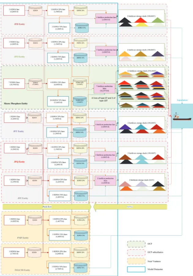
The time scale and the level of details captured by a model define its granularity. The perimeter of the studied productive system and the spatiotemporal granularity that is relevant to its operational steering, makes simulation modelling more appropriate than optimization where OR model cannot be solved in an acceptable run time to be used by managers during their weekly meeting of up to two hours. By choosing simulation, our research aims to model, by simulation, a hybrid supply chain for its operational steering. To clarify the modelling issues and show the value of our solution, we built our paper around a case study dealing with the management of OCP’s chemical plant at Jorf (http://www.ocpgroup.ma/en). This plant (illustrated in Figure 1) is one of the world’s largest and produces sulfuric acid and two phosphoric acids (29% and 54%), some fifty different fertilizers, with as many chemical nomenclatures. The industrial facilities combine multiple interconnected entities: an OCP division, five OCP subsidiaries and two JVs created in partnership with other countries. OCP extracts phosphoric ore upstream and transports it along a 235 km –long slurry pipeline, to feed the different phosphoric acid plants. These entities’ production lines for a particular product (acids, fertilizers), differ substantially in terms of yields and chemical nomenclatures.
While fertilizer shipments pull production, ore feeding pushes acids production. Phosphoric acid, that consumes sulfuric acid, is mainly used in fertilizer production (a small part of which is exported).While acid production involves continuous production, fertilizer production involves discrete production (one batch per Production Order (PO)). The real-time decisions mainly concern the physicochemical parameters of a continuous production line. This level of detail, and associated real-time decisions, are excluded from our scope. This has led us to consider each line as an independent processor to eliminate the micro decisions made to keep the process under control. We therefore gained a higher perspective of the process to achieve consistency between the relevant match between level of decision and continuous processes modelling detail (see Degoun, Fénies, Giard, Retmi, & Saadi, 2014).
Decision making for the 8 plants, comprising a total of some 80 production lines is partly independent and concerns: line openings, line production rates (adjusted at any time to accelerate or slow production down), scheduled preventive maintenance, schedule of fertilizer POs on fertilizer lines and scheduled exchanges of acid (monitored by valves) between entities. Every week, a steering committee assesses the consistency of these operational decisions (largely made locally), in order to implement the production program and avoid unplanned and very costly shutdowns. The spreadsheet approach
currently used by the committee has not delivered the expected results as some inconsistencies go undetected. On the other hand, our tests have shown the benefits of simulation for the steering committee’s purposes. Its implementation of course implied being able to properly simulate any HSC.
Figure 1: The Jorf chemical complex
Currently, neither Discrete Event Simulation (DES), the simulation tool most widely used by managers, nor System Dynamic (SD), are able to model and simulate such a HSC. We acknowledge that AnyLogic, a commercially available software combining
DES, SD and ABS (Agent Based Simulation) approaches (considered the most advanced software to model a HSC (Brailsford 2018)), delivers a number of functions to model continuous processes for operational decision-making purposes. This, however, has a number of limitations further discussed below. Our purpose is to describe a set of 4 components (in section 4), made up of two basic DES components: stocks and processors. These are designed to be easily implemented in all widely-used DES. These components enable the modelling and simulation of the relevant HSC. Measuring the impact of operational decisions on HSC, therefore, is our scientific contribution.
We devote section 2 to pointing out the differences between Discrete Processes (DP) and Continuous Processes (CP). This then enables us to list the issues we faced when seeking to model continuous processes with a DES. Section 3 sets forth our literature review. Unlike most researchers, we focused on HSC simulation rather than on hybrid simulation. Section 4 describes our set of four new generic components. These are made up of basic DES components and enable simulation of a complex HSC at the relevant level of granularity as defined above. Finally, section 5 discusses the feedback from the simulation performed with a DES using these components. Our aim is to assess the consistency of weekly operational decisions taken by the managers of the eight Jorf entities.
2. Issues arising when simulating a hybrid productive system
To form a clear pictures of the problems to be solved, one must fully grasp all the differences between discrete and continuous processes. Since our purpose is to enable the use of DES to simulate complex HSC, we analyse thereafter i) the issues involved in the flow discretization process used by some advanced DES software and ii) those induced by the transformation of a chemical nomenclature into a Bill Of Materials (BOM). In the last part of this section, we go on to highlighting the five issues to be solved in order to use a DES to model and simulate a hybrid complex supply chain adequately.
2.1 The difference between discrete and continuous processes
A discrete processor deals with physical entities (products, components…) indifferently called “items” in this paper by performing physical or spatial transformations (transportation). A Discrete Elementary Process (DEP) is operated by a discrete processor fed by one or more stocks in quantities governed by a BOM, during a given processing
time. The processor feeds one or more items to one or multiple stocks. Processor definition depends on the level of observation adopted and its use in the modelling.
Continuous Elementary Processes (CEP), on the other hand, transform flows (liquids, granules…) inside a continuous processor. The flows come from one or more stocks and the CEP feeds the output to one or more stocks. The rates of input and output streams correspond to the quantities defined by a chemical nomenclature. This depends on the performance of the processor as further described below. Under certain conditions, the average time during which incoming flows remain in the transformation process can be calculated analytically. This duration is similar to a processing time.
Turning to the discrete supply chains, we note that they comprise a network of DEPs linked i) by stocks (which can also be fed by one or several entry points) or ii) to productive system exit points. In the case of continuous supply chains they are made up of a CEP network. It follows that hybrid SCs is made of any combination of one or multiple DEP(s) with one or multiple CEP(s).
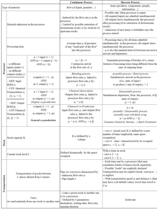
The problems involved in simulating a HSC entail specifying the differences between DEPs and CEPs in order to identify the issues to be solved when connecting DEPs with CEPs and vice-versa (CEPs with DEPs). To this end, a number of DEP and CEP characteristics must be taken into account: i) processor features (admission, processing time, impact of the BOM or of the chemical nomenclature), ii) stock features (offered capacity and used capacity) and iii) transportation (means and monitoring of transportation). Table 1 describes the different criteria, pertaining to DEPs and CEPs respectively, to be taken into account in the simulation. Some CEP notations are defined and illustrated below.
To be able to handle CEPs, DES software must transform a flow into a sequence of items. Though this is performed by some DES software claiming to simulate continuous processes, the result falls short of the mark as will be shown below. Before going into further detail, we must let us the discretization process.
Table 1: Main differences between a Continuous Process and a Discrete Process in simulation modelling
2.2 Preliminary transformations for modelling a CEP in a DES
To be able to deal with continuous flows in a DES, we had to define an appropriate flow discretization process and to transform our chemical Nomenclatures into Bills of Materials.
Discretization process
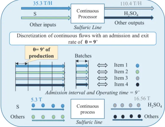
Flow discretization creates Continuous Items (CI) which inherit the chemical characteristics of the flow. CI volumetric and weight characteristics depend on input rate and on time interval θ which delimits the batch of liquid or granules associated with this CI. For instance (see Figure 2), let’s consider a discretization interval of = 9’ common to all inputs and outputs of a sulfuric line: the input of liquid sulphur in the CEP at a flow rate of 35.3 T/H generates each 9’ a liquid sulphur CI, weighing 35.3 (9/ 60) 5.3 T. Note that any subsequent flow rate change will also change CI weight. The CIs will be processed by discrete or continuous elementary processes.
Figure 2: Discretization of a continuous flow
Transformation of the Chemical Nomenclature into a Bill Of Materials
Typically, a continuous process picks a set of different inputs and produces different outputs. Let us consider the example of phosphoric acid production, which pertains to general co-production of Table 1. This uses the following molar equation (1) (supplemented by the indexes used in Table 1 and the atomic numbers of these molecules) which verifies the principle of mass conservation (sum equal to 364).
2 4 1 2 3 1 2 3H SO + i i i j j
sulfuric acid Phosphogypse Water Phosphoric acid Tricalcium phosphate
2 3 4 3 4 2 4 2 Ca (PO ) + 2 150 154 60 100 6H O 2 H PO + 3( 64 Ca SO ,2H O ) ( 1)
In these conditions, the chemical nomenclature is: α1150 / 364 0.41209 , 2
α 154 / 364 0.42308 , α360 / 364 0.16484 , β1100 / 364 0.27473 , 2
β 100 / 364 0.72527 .
With an entry interval of θ=60' and an hourly production rate of ρ 524.16 T/H for a phosphoric acid line, the process pulls every 60 minutes a CI of 524.16 0.41209 216 T of sulfuric acid, a Tricalcium phosphate CI of 221.76 T and a water CI of 86.4 T. Every 60 minutes, the process will push a phosphoric acid CI of 144 T and a phosphogypse CI of 380.16 T.
From the DEP point of view, the BOM lists the requirements to manufacture one unit of a given product. The BOM indicates that for each phosphoric acid (144 T) output item, one needs 1 sulfuric acid (216 T) input item, 1 Tricalcium phosphate input item (221.76 T) plus 1 water (86.4 T) input item. Naturally, as previously stated, the weight of these items depends on flow rate.
The four following key considerations concerning industrial production should be taken into account:
Theoretical BOMs are not feasible in an industrial context as they cannot yield optimal production conditions. To obtain periodic production of 144 T in actual industrial conditions one needs more inputs than those allowed by theoretical BOMs: (e.g., 217.08 T instead of 216 T of sulfuric acid). This additional input consumption, driven by actual industrial facilities, generates slags and gases, though the mass conservation principle, of course, is satisfied.
In most process industries, line capacity (often expressed as a flow rate for a given period) is defined for the main product for which the line was intended. Our example for a phosphoric acid line (j = 1), the hourly production rate is.
1
ρj 524.16 0.27473 144
. On the other hand, the chemical nomenclature is often defined by a ratio that is independent from production rate. For instance, for sulfuric acid the ratio is α1/β11.5, which means that the production of 1 T of
phosphoric acid requires 1.5 T of sulfuric acid. When multiplying that value by ρj1 , one gets sulfuric acid input flow rate ρi1ρj11.5 144 1.5 216.
If CI weights are defined by formulae θ×ρ α j and θ×ρ β k, then any flow rate change implemented during the simulation will also change these weights.
Once CIs are created, they can be used directly either by continuous processes or by discrete processes which treat them as “regular” items.
2.3 Additional issues involved in CP modelling by a DES
An analysis of Table 1 to compare the features of CP and DP brings up five issues related to the treatment of CIs as “normal discrete” items to be used by a DES software.
(1) Where a “discrete” processor is used as if it were a “continuous” processor with processing time , this implies that time interval between two successive CI entries (and departures) is equal to . This solution, used by some software (including AnyLogic) may trigger important artificial fluctuations in the simulation if is extended for some continuous processors. In that case the system will produce erroneous predictions of downstream stockout or saturation or upstream depletion, etc. For example, in our case study, processing time for sulfuric acid is 9’, whereas that for 29% phosphoric acid is 240’. To smooth the effects of discretization and obtain relevant simulation reports, one must therefore disconnect interval of entry into the processor from processing time , if is too long. To achieve this disconnection, one will feed the processor at an interval of <, where (preferably common to all CEPs) must be short enough to enable the simulation to produce relevant reports. Where interval is around 10’, discretization time is short enough to adequately iron out the fluctuations induced by modelling a CEP in a DES. The additional effects of replacing by include: i) a change in input and output weights handled by the processor; ii) doing away with traditional use of a DES processor since it cannot accept new inputs as long as it has not completed work in progress. We describe in section 4 the solution we worked out to solve this problem. It should be noted that the above-described adaptation to include a continuous process into a DES does not impact DEP modelling.
(2) The second issue concerns stock capacity, usually defined by the maximum number of items it can contain. This is relevant only if items have the same volume or weight (depending on the way capacity is defined). Since a given stock may be fed by CIs coming from continuous processors whose flow rates differ, the CIs must be considered as heterogeneous. Some DES software may define current stock occupation in volume or weight, sometimes by aggregating all items into a single one. In the latter case, there is no stock capacity issue, otherwise a capacity stock (we name “Tank”) generic component must be created.
(3) The third issue stems from the unavoidable variation of particular CI weight requirements (e.g. sulfuric acid) by processors. If the capacity stock uses a single aggregate item, then a new component must be created to extract a CI with the required weight and update stock capacity. Otherwise, another component must be created to pull and aggregate CIs from the stock to satisfy requirements and return to the stock a CI accounting for unused excess weight. To illustrate this issue, let’s take the case of a sulfuric acid plant comprising six identical lines, whose nominal production rates are 110 T/H with processing time = 9’ (where =), and sulfuric CIs of 11 T (at nominal production rate). Four lines out of the six comprising the phosphoric acid plant have a nominal production rate of 144 T/H. One line has a nominal production rate of 79 T/H and the remaining line, a production rate of 107 T/H. Since processing time is =240’, we use entry interval = 60’. This means that the first 4 lines will require 216 T of sulfuric acid CI requirements (as calculated above) and the other 2 will need 118.5 T and 160.5 T respectively. These values will of course vary if, during the simulation, one decides to modify the nominal rates that were initially defined. We obviously need to introduce a component between the stock and the processor to obtain CIs of required weight. Turning to the treatment enabled by AnyLogic, we note that the component used to model a continuous process may be linked by up to 5 converters to upstream stocks. The main limit is that one may not link a converter to several upstream stocks of the same product.
(4) In DES, stocks cannot be directly linked because they behave passively. In order to use a DES to simulate a hybrid SC, a valve component must be created to manage multiple flow exchanges at both predefined dates and given rates. While AnyLogic offers such a possibility it uses fixed expected start and end dates. In the case of a transfer program lasting several days, however, the expected dates (per transfer) may change as a result of unforeseen incidents. Addressing this issue calls for fairly
complicated code instructions: another component is added to simulate such scenario through Java coding.
(5) The last issue corresponds to the situation where part of the supply chain is pulled by demand. This means that one must be able to drive a portion of continuous production with a Production Order. Such synchronization problems between information and production flows also occur in discrete production. In continuous production, however, they are trickier to deal with. Returning to AnyLogic, its representation of continuous processes is limited to a single product output whose weight characteristics must be maintained throughout the simulation period. Additionally, the output's weight may not be changed when switching from one PO to another. As a result modelling of a multi-product line requires recourse to as many processors as there are POs. This software, therefore is not suited to cases characterized by strong diversity such as our fertilizer production line example nor where speed changes to line operations may be required during simulation. Note that our set of generic components is easy to implement in that software.
Section 4 is dedicated to describing our solutions to solve these 5 issues.
3. Literature review
After a brief review of the three main simulation approaches, which are well known, we will take stock of their ability to simulate the behaviour of a complex hybrid productive system. We define such a complex system as comprising any combination of CDPs and DEPs in co-production, responding to a set of operational decisions. We shall focus on the simulation system’s ability to deal with this kind of decision-making in the relevant type of productive system. We will then assess the ability of the most advanced hybrid simulation software to solve our problem. We shall then turn to what the experts say about commercial software and summarize their main conclusions drawn from the excellent surveys recently published. Furthermore, we report previous propositions for the modelling of a HSC with DES. Finally, we show that these observations entirely support our approach.
3.1 Main simulation approaches
Discrete Events Simulation
According to Brailsford, Churilov and Dangerfield (2014, chapter 6), “DES models systems as networks of queues and activities, where state changes in the system occur at discrete points of time. The objects in the system are distinct individuals, each possessing characteristics that determine what happens to that individual, and the activity durations are sampled for each individual from probability distributions”. DES is best suited to study operational and tactical decisions (Andersson & Olsson, 1998; Borshchev & Filippov, 2004; Jeon & Kim, 2016). It enables a productive system representation at the relevant granularity (space, time…) to assess the impact of decisions that are going to be applied.
System Dynamics
Brailsford et al . (2014, chapter 6) define system dynamics models as a “network of stocks and flows, in which the state changes are continuous. The processed objects are mainly continuous quantities (fluids…) that circulate in a system of tanks linked by pipes”. SD focuses on policies rather than decisions. It models system changes where flows circulate and their evolution is described through differential equations. SD models the SC at a high level of aggregation, by considering aggregate quantities and not individual entities, and yields a macroscopic view of the functioning of the system at hand (Brailsford et al., 2014, chapter 3; Jeon & Kim, 2016; Kleijnen, 2005; Scholz-Reiter, Freitag, Beer & Jagalski, 2005; Venkateswaran & Son, 2004;). Despite its usefulness to clarify the complexities of organizational behaviour, SD has limitations including a simplified representation of systems, the need to aggregate entities, and the use of average flow rates. On the other hand, DES offers much more of flexibility and provides sufficient details of the modelled system (Brailsford et al, 2014, chapter 6). Pertinent comparisons between the DES and SD are available in (Brailsford et al, 2014, tables 6.3, 9.1 and 9.3).
Agent-Based simulation
We have discarded the Agent-Based Simulation (ABS) approach, whose software offering is quite large (Abar, Theodoropoulos, Lemarinier & O’Hare, 2017), because this
modelling approach is not appropriate for the problem at hand. Agents, that may be used to represent products and resources are “objects with attitudes” (Bradshaw, 1997), capable of making autonomous decisions. As clarified by Aldea et al. (2004), “in a multi-agent system, multi-agents interact with one another to achieve their individual objectives by exchanging information, cooperating to achieve common objectives or negotiating to resolve conflicts”. A survey done by Jeon and Kim, (2016) showed that ABS is suitable for interrelationship issues where agents are used to represent the different SC players (supplier, manufacturer, supplier…). Detailed differences between DES and ABS are perfectly pointed out and summarized in excellent comparison tables in (Siebers, Macal, Garnett, Buxton & Pidd, 2010; Baldwin, Sauser & Cloutier 2015; Jeon & Kim, 2016). Borshchev and Filippov, (2004) and Jeon and Kim, (2016) underline that ABS is a decentralized and bottom-up modelling, whereas DES is centralized and top-down. In the kind of problem studied here, the behaviour of the entire simulated productive system results from a set of decisions taken once and for all, the production centres applying these decisions passively. The simulation purpose is to verify whether the productive system remains under control; if not, initial decisions are changed and their consistency is studied again through the same simulation model.
3.2 Hybrid simulation
Hybrid simulation (HS) may be defined by Jahangirian, Eldabi, Naseer, Stergioulas & Young, (2010) as “models that combine at least two of these three approaches to model complex enterprise-wide systems”. Brailsford et al. (2018), continuing Jahangirian et al’s work. (2010), have proposed an extensive HS survey. They have used the combination simulation typology of (Morgan, Howick & Belton, 2017), which enriches the traditional typology of OR tool combination proposed by Bennett, (1985): i) Sequential : two or more distinct single-method models that are executed sequentially (but only once), the output of one becoming the input of the following one; ii) Enriching: a dominant method, with limited use of other encapsulated method(s); iii) Interaction: distinct but equally important single-method submodels that interact cyclically during execution; iv)
Integration: “a seamless model in which it is impossible to tell where one method ends
and another begins”. In their survey of 104 papers dealing with HS, they found only 4 truly integrated models, all coded in bespoke software.
From our perspective, the issue to be solved is not to combine DES with SD, which is a hybrid simulation design problem, but to find an easy way of modelling and simulating a complex hybrid productive system to test the impact of operational decisions. Our approach is therefore quite different even though the bespoke integration software somewhat shares this objective.
3.3 Commercial software
In their extended HS survey, Brailsford, Eldabi, Kunc, Mustafee & Osorio, (2018) have analyzed commercial software. They claim that, although some SD software are able to use probabilistic sampling and some DES components (conveyor) and some DES tools provide a limited facility to model continuous flows and then represent some SD features, the integration is not exhaustive. This is “due to the fundamental differences between DES and SD in terms of model execution and the underlying methodological and theoretical assumptions, such as discrete versus continuous state change, or conceptualizing a system as a network of queues and activities rather than one of stocks and flows. Software that is implemented primarily as a SD or a DES tool will inherit not only the strengths but also the limitations of the underlying modelling method (Brailsford
et al. 2018)”.
3.4 Modelling Hybrid Supply Chain with Discrete Event Simulation
We have found examples in the literature of use of DES to model a hybrid SC (Chen, Lee & Selikson, 2002). Some entry points introduce in the hybrid SC, at regular intervals, CIs corresponding to batches of liquid or granule. This fragmentation, typically, corresponds to packaging (package, bag, truck…) used by transport. Subsequently, the CIs circulating in the hybrid SC are no longer processed by a CEP or can do so via a batch processing performed by a DEP; in the latter case, the size of the required batches is necessarily equal to the size of the CIs produced upstream.
Meyer et al, (2011) have modeled the hybrid SC of fuel production by using an approach based on separate DEP models: one model dedicated to gas factories and the other dedicated to fuel production. To produce gases or liquids the inputs are added to the reactor by batches. The batches issued by the first process are inputs to the second process. Following processing, the volumetric characteristics of the batches produced by the first process do not fit the requirements of the next one. This precisely corresponds to the third
methodological problem (section 2) that precludes use of DES in Hybrid SC without adjustment.
3.5 Conclusion
Our analysis of the literature shows that current DS, ABS and SED alone cannot meet the requirement of simulating hybrid complex systems where DEPs and CEPs interact, at the relevant operational level. Additionally, hybrid simulation using an integration approach involves major coding effort. The next section of our paper is dedicated to describing a set of generic components that are easily created in most DES. These generic components are complementary and enable the modelling of any kind of hybrid SC as part of a single model with a sufficient level of detail to analyse consequences of operational decisions. We did not find previous works presenting or explaining how to use a “traditional DES” to model an entire complex hybrid SC, in a single model, for its operational steering.
4. Principles of continuous SC modelling using a DES
This section describes a set of 4 generic components, made up of DES basic components (queues, processors). The exercise involves limited coding and answers the five issues arising when seeking to adapt DES to model CEPs (see section 2). The most widely used commercial software enable such component creation used as building blocks to develop a new model. The logical basis of some of these components was previously introduced by Degoun, Fénies, Giard, Retmi & Saadi, (2015).
Most DES software use a large library of such pre-defined building blocks, corresponding to basic components to model a process without requiring any custom programming. Their icon representation is dragged and dropped on the screen to create the representation of the productive system and the possible routes between these objects. In a generic perspective, independent of any DES software, our generic components creation relies on two basic components: the processor (that transforms an item) and the stock (where an item may stay without being processed). Most DES tools offer coding possibilities featuring the properties of items or basic components and can access information stored in simulator spreadsheets. For our purposes, we characterize items, stocks and processors using labels accessible through the following conventions: “item.label”, “stock.label” and “processor.label”. Additionally, the “stock” and
“processor” basic components may be used in an unconventional way when they are included in one of these generic components; in that case, we call them “dummy”. 4.1 The ‘Continuous Process’ generic component
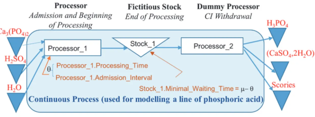
We propose a continuous process generic component (see Figure 3) by combining three basic DES elementary components, “perverted” to suit our purpose.
Upstream, a stock is fed by a processor (‘Processor_1’, in Figure 3), whose processing time θ corresponds to both the CIs entry interval and the beginning of their processing time (μ θ) . The processor is connected to stocks of different inputs through ‘converters’ and picks an item from each stock according to the BOM (see section 2). In Figure 3, the three stocks for the products are those required for phosphoric acid production.
Downstream, this processor is connected to a fictitious stock (‘Stock_1’), with a retention time of μ θ corresponding to the residual processing time. This allows the presence of items at different stages of production progress in the continuous process. Downstream, the stock is connected to a dummy processor, ‘Processor_2’, whose function is to extract from the fictitious stock any CI having remained there during the minimum sojourn time μ θ . Typically, once the operation is complete, several items of different nature are transferred to as many stocks, as per the BOM. These stocks generally have limited capacity.
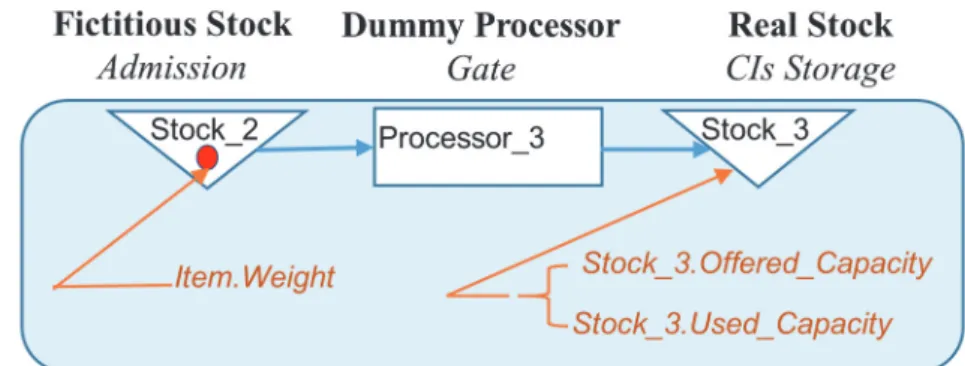
4.2 The ‘Tank’ generic component
We have seen in section 2 that, in DES, stock capacity is usually expressed by a maximal number of items that it can contain. In some software, it is possible to define it as a maximal volume (or weight) it can contain, which is useful in case of heterogeneity of items volume or weight. To address this issue, we designed the ‘Tank’ generic component that combines (see Figure 4) three basic components, a dummy processor, a dummy stock and a real stock. A tank is characterized by labels ‘Stock_3.Offered_Capacity’ and ‘Stock_3.Used_Capacity’, whose values are expressed in weight (or volume) and initialized when resetting the simulation. The first label is static and keeps its initial value during the simulation, while the second varies dynamically, depending on the incoming and outgoing items. Items are characterized by the ‘Item.Weight’ label.
Figure 4: The ‘Tank’ Generic component
Dummy stock ‘Stock_2’ can store a maximal number of CIs equal to the number of processors feeding that ‘tank’ (and not always one, to avoid possible upstream unpriming problems).
Dummy processor ‘Processor_3’ only accepts items if the residual capacity of the ‘real stock’ is sufficient. That is guaranteed by the following program run before the item is picked up in ‘Processor_3’.
If Stock_3.Used_Capacity+Item.Weight < Stock_3.Offered_Capacity Then admit item in Processor_3
If not Block item picking
Upon entry of an item in the “real” stock, ‘Stock_ 3’, used up capacity is updated by the following program:
Upon exit of an item from this stock, used up capacity is updated by the following program
Stock_3.Used_Capacity Stock_3.Used_Capacity - Item.Weight
A tank can be fed by other tanks or by CPs. A CP which delivers outputs that feed tanks must stop functioning as soon as one of these stocks is saturated. The solution involves introducing a program inspired from the above-described test to block CP supply (e.g., performed upon entry into ‘Processor_1’ of Figure 3). Production shutdown due to downstream stock saturation is very difficult to forecast without recourse to simulation. 4.3 The ‘Converter’ generic component
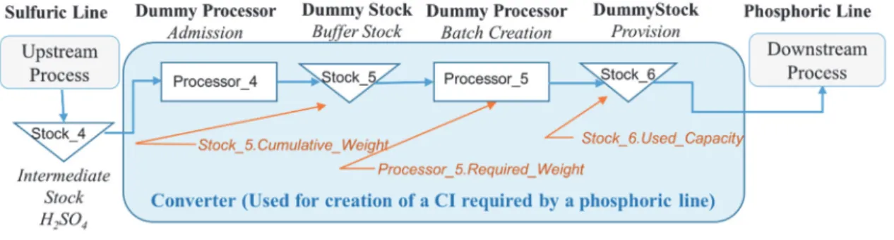
The third issue detailed in section 2 deals with the fact that coupling two CPs linked by a stock is impossible if the weight of the items produced upstream differs from that required downstream. By resorting to a ‘Converter’ generic component comprising four basic components (two dummy processors and two fictitious stocks), one is able to create an item matching the required downstream weight.
Figure 5: The ‘Converter” generic component
‘Stock_6’ receives a CI having the required weight downstream. This stock has a unit capacity to ensure that the conversion process follows any change in downstream requirements. It is characterized by the ’Stock_6.Used_Capacity’ Label.
‘Stock_5’ receives items that enter into the composition of the item having the required weight. This stock, characterized by the labels ‘Stock_5.Cumulative_Weight’ and ’Stock_5.Number.Items’. Arrivals in ’Stock_5’, trigger the following program:
Dummy ‘Processor_4’ picks up CIs from ‘Stock_4’ to push them to ‘Stock_5’, provided ’Stock_6’ is empty and ‘Stock_5.Cumulative_Weight’ is below the required weight recorded in the label ‘Processor_5.Required_Weight’ (which is updated dynamically as production goes on). These conditions are monitored by the following program run before entry into ‘Processor_4’:
If Stock_6.Used_Capacity =1 then Block item picking
If Stock_5.Cumulative_Weight ≥ Processor_5.Required_Weight then Block item picking
Dummy ‘Processor_5’ extracts CIs from ‘Stock_5’ and merges them as soon as ‘Stock_5.Cumulative_Weight’ exceeds ‘Processor_5.Required_Weight’ and ‘Stock_6’ is empty. These conditions are monitored by the following program, run before entry into ‘Processor_5’ that uses a local parameter k.
k 0
If Stock_6.Used_Capacity =1 then k 1
If Stock_5.Cumulative_Weight <Processor_5.Required_Weight then k 1
If k=1 then Block item picking
If not:
Pick all the items from Stock_5 and merge them into a single item whose Item.Weight Stock_5.Cumulative_Weight - Processor_5.Required_Weight Stock_5 : Stock_5.Cumulative_Weight Stock_5.Cumulative_Weight
Processor_5.Required_Weight
As a result, ’Processor_5’ delivers two identical CIs, one of which is sent to ’Stock_5’ and the other to ’Stock_6’. When the CI enters ’Stock_6’ the following program is run:
Item.Weight Processor_5.Required_Weight
The ‘continuous process’ and ‘converter’ generic components enable the successful modelling, through a DES, of any linked processors performing coproduction (as defined in Table 1). It follows from the above that our generic components are complementary. Indeed, the development of the next generic components relies on two of the three previous generic components in addition to other basic components.
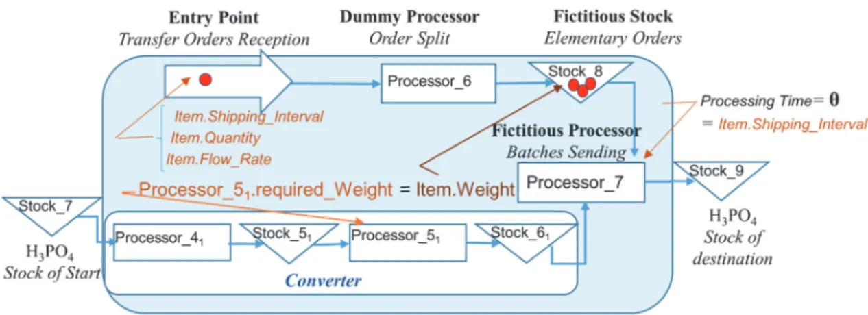
4.4 The ‘valve’ generic component
We now turn to pull-flow control which requires synchronization with an information flow (manufacturing orders…). CI transfers from one stock to another implies recourse to a valve and results from a transfer decision at a date, for a given quantity and at a given
flow rate. The ‘valve’ generic component (Figure 6) activates a converter, an entry point, a dummy stock (’Stock_8’), a processor (‘Processor_7’) and a dummy processor (’Processor_6’).
Figure 6: The ‘Valve’ generic component
The Entry Point is used to introduce items that correspond to flow transfer orders from ’Stock_7’ to ’Stock_9’. Labels ’Item.Quantity’, ‘Item.Flow_Rate’ and ‘Item.Shipping_Interval’ are read from a table and assigned to the incoming item through the Entry Point.
Dummy ’Processor_6’ operates at the transfer starting date. It splits the incoming item (transfer order) into m items on exit, corresponding to elementary shipping orders. This number m is calculated by running the following program upon item entry:
m Rounded[Item.Quantity/Item.Flow_Rate]
The Item.Weight of the outgoing items and ‘Processor _5.Required_Weight used by the ‘converter’ which prepares the required CI, are defined by:
Item.Weight Item.Quantity/m
Processor_5.Required_Weight Item.Quantity/m
‘Processor_7’ merges items taken from ‘Stock_7’ (information) and from ‘Stock_6’ (material). ‘Processor_7’ processing time θ takes the value of ‘Item.Shipping_Interval’.
4.5 Modelling the management of continuous process by production orders
We now describe the solution for the type of generic problem that does not use a generic component but a simple approach relying on the three first generic components. We illustrate it with fertilizer orders. Our example draws on situations from the Jorf fertilizer
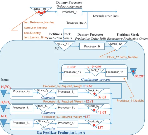
plant which comprises multiple parallel production lines. The order book containing the assignment of orders to production lines is an input of the simulation model. Orders are assigned to a line in a predetermined sequence and processing starts as soon as possible, subject to the setup times between two successive fertilizer productions. In our case study, we use an information gathering interval of one hour. As the processing time is of several hours and the production of a fertilizer PO may require several hours (up to 1 day, sometimes more), one must split each PO into small elementary POs, whose CI weight corresponds to one hour of production, and represent the fertilizer process with our generic component “Continuous Process” (Figure 7). The modelling of such a pull-flow production is illustrated by Figure 7, which represents a single line.
Figure 7: Modelling a fertilizer line (using 3 converters) governed by a pull system When starting simulation, ‘Stock_10’ content is initialized with a number of items
equal to the number of orders to be processed. Each order is characterized by the reference to be produced: ‘Item.Reference_Number’, its assigned line,
‘Item.Line_Number’, the quantity to be produced, ‘Item.Quantity’ and set-up time, ‘Item.Launch_Time’, before starting production. The FIFO order of items matches the production sequence.
Dummy ‘Processor_8’ sorts orders and sends them to the appropriate line orders queue via label ‘Item.Line_Number’. Line A is assigned Stock_11.
Dummy ‘Processor_9’ splits each manufacturing order into n elementary orders. This number is calculated as the rounded-up value of the quotient of the quantity to be produced (e.g. 11.640 T) by the production line rate (e.g. 1.347 T/minute), multiplied by the entry time interval θ (e.g. 60'). In our example the manufacturing order of 11.640 T is split into 11640 / (60 1.347) 145 elementary orders characterized by weight 11640 /145 80.28 T. ‘Processor_9’ can accept new items only if stock_12 has available space.
With the entry interval θ =60’, ‘Processor_10’, which governs the continuous process, picks an elementary order (information) from ‘Stock_12’ and extracts from ‘Stock_62’, ‘Stock_63’ and ‘Stock_64’ the items (materials) corresponding to the
necessary inputs (acids…). The CIs correspond to the inputs used to produce 80.28 T, according to their BOM (37.6 T of phosphoric acid, 54.13 T of ammoniac and 12.8 T of sulfuric acid). The ‘Processor_11’ delivers, each 60’, an output item whose weight is ‘Processor_11.Output_Weight’.
Note that, at this stage, we ignore updating of the entry interval θ and of processing time μ which may depend on ongoing routing and can be deducted from line number and fertilizer id. As BOM and routing of two successive orders on the same line may differ, updating input weights of the continuous process is required immediately after entry of a new item into ‘Processor_9’ by running the following program:
Read Item.Reference_Number
If the reference to be produced is different from the ongoing reference Then Update: Processeur_52.Required_Weight,
Processeur_53. Required_Weight, Processeur_54. Required_Weight Processor_11.Output_Weight
5. Case study
In the introduction, we described the characteristics of the productive system at hand and the operational decisions to be built into the simulation. In the first part of this section,
we briefly describe the use of generic components in model building. Under the second part, we go on to discussing some of the valuable lessons drawn from the simulation exercise.
5.1 Simulator development and characteristics
The use of generic components in modelling the productive system (by using the DES software Simul8) is described in Table 2. A hierarchical modelling approach was used: for instance, the generic components combination, used to describe the fertilizer production line (see Figure 7), is combined into a super-component which is duplicated to model any line within the fertilizer plant. Generic component parametrization is performed through an Excel spreadsheet loaded before launching the simulation. This parametrization ensures that the model is easily maintained and to accommodate any possible extension as a result of future integration of new entities.
Table 2: Generic component occurrences in the Jorf model
We adopted an information gathering interval of 60’. Accordingly, where μ 60' , we use an entry interval θ 60' , otherwise θ=μ . The information gathering interval gives us early warning of any incident occurring during a period (one hour in this instance) rather than exact occurrence time. Although an interval of less than 1 hour could have been used, it had little added value in our case and simply slowed the simulation down.
Usually, managers take decisions within a two to three weeks horizon. The simulation is therefore performed over the same horizon to predict the productive system performance by providing, for each stock and production line, the status and changes using an hourly scale. The results of a two-week scenario are obtained after a run time of 4 minutes in a computer of following characteristics (Intel ® Core(TM) i7-7600U CPU @ 2.80GHz 2.90GHz – 8 Go (RAM))
5.2 Simulator validation
At the time when we performed the validation, our model was limited to the largest entity, Morocco Phosphore (Figure 1). It was subsequently extended to include the other entities. As mentioned above, Jorf’s steering committee used spreadsheets to ensure the set of
incoming operational decisions actually delivers the required production. This instrumentation requires time for data input and processing and involves redundant inputs without consistency checking. Such an approach is not efficient to detect the propagation in time and space of the impact on the supply chain of a set of decisions. As a consequence, Jorf managers have to solve unforeseen problems, both locally and, later, upstream or downstream as a result of their propagation along the SC.
We performed several comparisons between actual results and those predicted by our model (by tracking production and stock changes). They revealed that the simulator reliably reproduced Maroc Phosphore operations and spotted existing inconsistencies. The latter generally stemmed from unplanned shut-downs due to upstream stock-out, or, more frequently, downstream stock saturation (and subsequent upstream propagation). Where inconsistencies were detected, the simulator also provided decision support with a rapid scanning of alternative sets of decisions tested using the same model. The process was reiterated until consistency was reached. For instance, in the case of phosphoric acid 29% stock saturation, the simulator recommended either to: i) decrease production rate for some acid lines, or change ii) the maintenance program, iii) transfer acid between entities, iv) or adjust the fertilizer PO schedule (which impacts acid consumption).
To conclude, our model successfully predicted the functioning of the productive system in response to local decisions by managers of different units. It therefore helped the steering committee negotiate alternative decisions with them to restore decision consistency and, thus, avoid some costly emergency decisions.
6. Conclusion
The generic DES solution described in this paper is easily implemented in the most widely available DESs. It successfully models and simulates hybrid supply chains made up of any combination of continuous and discrete processes, including coproduction ones, in response to a set of operational decisions. This solution was tested in a major chemical complex in order to study the consistency between a set of operational decisions taken by managers of several interdependent entities. In case of inconsistencies, the simulator provide them with better alternative decisions. The opportunity of its adoption by the steering committee is being reviewed.
7. References
Abar, S., Theodoropoulos. G., Lemarinier, P., & O’Hare, G.M.P. (2017). Agent Based Modelling and Simulation tools: A review of the state-of-art software. Computer
Science Review, 24,13-33.
Aldea, A., Bañares-Alcántara, R., Jiménez, L., Moreno, A., Martı́nez, J., & Riaño, D. (2004). The scope of application of multi-agent systems in the process industry: three case studies. Expert Systems with Applications, 26, 39-47.
Andersson, M., & Olsson, G. (1998, December). A simulation based decision support approach for operational capacity planning in a customer order driven assembly line. Proceedings of the 30th conference on Winter simulation, (pp. 935-942). Washington, USA, IEEE.
Baldwin, W.C., Sauser, B., & Cloutier, R. (2015). Simulation Approaches for System of Systems: Events-based versus Agent Based Modeling. Procedia Computer
Science, 44. 363-372.
Bennett, G. (1985). On Linking Approaches to Decision-Aiding: Issues and Prospects.
Journal of the Operational Research Society, 36, 659-669.
Bradshaw, J.M. (1997). An Introduction to Software Agents. Software Agents, 4, 3-46. Brailsford, S., Churilov, L., & Dangerfield, B. (2014). Discrete-Event Simulation and
System Dynamics for management decision making. Wiley (Series in Operations
Research and Management Science).
Brailsford, S., Eldabi, T., Kunc, M., Mustafee, N., & Osorio, A.F. (2018). Hybrid simulation modelling in operational research: A state-of-the-art review. European
Journal of Operational Research, 278, 721-737.
Borshchev, A., & Alexei, F. (2004). From System Dynamics and Discrete Event to Practical Agent Based Modeling: Reasons, Techniques, Tools. The 22nd
International Conference of the System Dynamics Society, Oxford, England,
Chen, E.J., Lee, Y.M., & Selikson, P. L. (2002). A simulation study of logistics activities in a chemical plant , Simulation Modelling Practice and Theory, 10, 235–245. Degoun, M., Fénies, P., Giard, V., Retmi, K., & Saadi, J. (2014). General Use of the
Routing Concept for Supply Chain Modeling Purposes: The Case of OCP S.A.
APMS 2014 (Advances in Production Management Systems), in Advances in Production Management Systems: Innovative and Knowledge-Based Production Management in a Global-Local World, Grabot, B., Vallespir, B., Samuel, G.,
Bouras, A., Kiritsis, D. (Eds.) 323-333, Springer, Berlin, Heidelberg
Degoun, M., Fénies, P., Giard, V., Retmi, K., & Saadi, J. (2015). “Propositions de règles de modélisation pour une simulation discrète d’une chaîne logistique hybride” [Proposal of modelling rules for a discrete simulation of a hybrid supply chain ].
Congrès international du génie industriel (CIGI2015). Québéc, Canada.
Jahangirian, M., Eldabi, T., Naseer, A., Stergioulas, L.K., & Young, T. (2010). Simulation in manufacturing and business: A review. European Journal of
Operational Research 203, 1-13.
Jeon, S.M., & Kim, G. (2014). A survey of simulation modeling techniques in production planning and control (PPC). Production Planning & Control, 27, 360-377. Kleijnen, J. P. (2005). Supply chain simulation tools and techniques: a survey.
International Journal of Simulation and Process Modelling, 1, 82–89.
Meyer, M., Robinson, H., Fisher, M., Van der Merwe, A., Streicher, G., Van Rensburg, J.J…Bonthuys, G., (2011). Innovative decision support in a petrochemical production environment, Interfaces, 41, 79–92.
Event Simulation and System Dynamics. European Journal of Operational
Research, 257, 907-918.
Scholz-Reiter, B., Freitag, M., De Beer, C., & Jagalski, T. (2005). Modelling dynamics of autonomous logistic processes: Discrete-event versus continuous approaches.
CIRP Annals-Manufacturing Technology, 54, 413–416.
Siebers. P.O., Macal, C.M., Garnett, J., Buxton, D., & Pidd, M. (2010). Discrete-event simulation is dead, long live agent-based simulation!. Journal of Simulation, 4, 204-210.
Venkateswaran, J., 1Son, Y.J. (2004). Distributed and hybrid simulations for manufacturing systems and integrated enterprise. in IIE Annual Conference.