09-00
7
Research Group: Development
January, 2009
Risk Taking of HIV-Infection and
Income Uncertainty: Empirical
Evidence from Sub-Saharan Africa
Risk Taking of HIV-Infection and Income
Uncertainty: Empirical Evidence from
Sub-Saharan Africa
∗
Elodie DJEMAI
†Toulouse School of Economics - ARQADE
This version: January 2009
First draft: April 2008
Abstract
This paper questions the positive relationship between HIV prevalence and income in Sub-Saharan Africa. In this paper, we hypothesize that a greater economic instability would reduce the incentives to engage in self-protective behaviors inducing people to increasingly take the risk of HIV-infection and hence causing a rise in HIV prevalence. We provide a simple model to stress on the effects of an increase in income risk in the incentives for protection. We test the prediction using a panel of Sub-Saharan African countries over the period 1980-2001. It is shown that the epidemic is widespread in countries that experience a great instability in gross domestic product over the whole period. When introducing income instability, GDP per capita is devoid of predictive power and the puzzle of the positive relationship between income and prevalence in Africa is lifted. Additional finding states that the risk taking of HIV-infection increases when the individuals are facing frequent and large crop shocks.
∗Special thanks to Jean-Paul Azam. I am grateful to Hippolyte d’Albis, Zi´e Ballo, Pierre Dubois,
Juan Miguel Gallego, C´eline Nauges, Franck Portier and participants at the Second Riccardo Faini
Doctoral Conference on Development Economics and at the Health Econometrics Workshop (2008) for valuable comments on previous versions of the paper. The usual disclaimer applies.
†Toulouse School of Economics (ARQADE), Manufacture des Tabacs, MA103, 21 all´ee de
1
Introduction
The HIV/AIDS epidemic exhibits complex patterns because the epidemic affects poorer countries worldwide, but amongst Sub-Saharan countries the richer ones experience the greater prevalence. 0.8% of the global adult population was living with HIV/AIDS in 2001 (UNAIDS 2007). This average prevalence was not reached in the two richest regions since in Western and Central Europe and in North America, 0.2% and 0.6% of the adult population were HIV-infected respectively. But the levels of prevalence in Sub-Saharan Africa clearly exceed the global estimate since there, the average prevalence reached 9.44% in 2001. Concerning the flow of new infections, one estimates that in 2004, over the 4.9 millions of new contaminations, more than 95% occur in low and middle-income countries (UNAIDS 2004). By contrast, a close look at the spread of the epidemic within Sub-Saharan Africa reveals that the richest regions are the most hit by the epidemic. Indeed, in 2001, Southern Africa was the most affected region with 23.5% of the adult people living with HIV/AIDS, followed by Central Africa with 7.20%, East Africa with 5.11% and lastly West Africa with 4.30% of its adult population infected.
A series of studies documents the sensitivity of the HIV/AIDS epidemic to in-come at both macroeconomic and microeconomic levels. In Sub-Saharan Africa, macroeconomic evidence claims that the national HIV prevalence levels increase with wealth (Bloom et al 2001; Clark and Vencatachellum 2003; Lachaud 2007). In a couple of African countries, empirical works suggest that rich individuals are more likely to be HIV-infected or to engage in risky sexual behaviors than their counter-parts (Kazianga 2004; de Walque 2006; Lachaud 2007). Traditional literature related with the investment in health suggests that the investment increases with the in-come level while in the particular case of the HIV/AIDS epidemic in Africa, things go on the opposite direction. People adopt risky attitudes that reduce their hu-man capital as their income increases. In Sub-Saharan Africa, the relation between epidemic and income is puzzling. Clark and Vencatachellum (2003) solve this appar-ently counter-intuitive relation for the industrialized countries within Sub-Saharan Africa.
By contrast, this paper introduces the economic uncertainty to complete the puzzle. In Africa, the widespread instability and the lack of protection against the occurrence of exogenous risks and against their negative consequences might
influence the individual choice and attitudes toward the risk of infection, and namely, might reduce the value people grant to the risk of infection. Here we focus on the risky sexual behaviors but any investment in health and human capital might be influenced by the widespread instability of the revenues. It is worth thinking of some recent cases in which people lost all they owned from day to day as in the
conflict outbreak in Cˆote d’Ivoire and in Darfour or as in the wave of expropriation
undertaken in Zimbabwe. Even rich individuals are likely to change their viewpoint concerning the risk of infection when they face such an event. Without referring to such extreme cases, agriculture is well-known as the activity that is dominant in most African countries and vulnerable to the climate. Once a farmer has planted his crop and is waiting for harvest, he is able to anticipate how good the harvest will be in the following months. If he experiences a drought, a damaging rainfall variation or even a locust invasion, he knows that his harvest will be bad and the prospects to sell it on the market or to stock it in his granary are thin. In such a context where the priority is to satisfy the primary needs, an individual who usually opts for safe sex may engage in unsafe sex one day either ex-post or ex-ante a risk on his own income. More broadly, living in a country of high economic instability might not encourage the agent to adopt safe sexual behaviors because it is not sure that in the future, he will be in good living conditions. A similar desincentive mechanism operates for the employee who has to exert much effort to get promoted in the sense that if the exogenous probability that his firm will go bankrupt in the following period is high, he has no incentive to exert any effort. In the context of the HIV/AIDS epidemic, the reasoning is the same, why should people engage in safer sexual practices to be sure to live longer and healthy when they are not sure that they will live in good conditions? Anticipating exciting future prospects will on the contrary encourage them to invest in self-protection. The bottom line of the paper is to argue that individuals must face so many risks in their everyday life that actually they do not care to take one additional and deliberated risk. We argue that whether the economic shock is anticipated or contemporaneous to the decision, the bottom line is maintained.
In this vein, we question the positive relationship between HIV prevalence and income in Sub-Saharan Africa and test the incidence of the aggregate economic risks faced by the individuals on their choice between safe and unsafe sex and hence on the spread of the epidemic. These interactions have not yet been explored in the
literature and provide a potential explanation for the low incentives to opt for safer behaviors in Sub-Saharan Africa. We propose a simple model of individual choice under the HIV/AIDS epidemic to gain insights about the mechanisms at stake. The prediction derived from the model is that for a given average income, an increase in the income risk reduces the incentives to choose self-protection. Empirical findings validate this prediction. Using a panel data of Sub-Saharan African countries over the last two decades, results suggest that the volatility in gross domestic product influences the spread of the HIV/AIDS epidemic. The more unstable the economies, the higher are the levels of prevalence. We uncover that the instability of the GDP per capita has distinguishable effects according to the income group in some esti-mations. Extracting the cyclical component of the GDP shows that taken alone the income may lead to a spurious relation between income and prevalence in the sense that it includes both the trend and the fluctuations. When introducing the measure of GDP instability, GDP is devoid of its predictive power and the puzzle is lifted. The effect of crop shocks on the spread of the epidemic is analyzed as an extension and confirms the benchmark results.
The paper is organized as follows. Section 2 presents the background of the problem and develops a model of individual choice between safe and unsafe sex to highlight how income instability alters the incentives to invest in self-protection. This theoretical framework aims to shed some light on the microeconomic founda-tions that are behind our empirical investigafounda-tions. Section 3 presents the indicator of economic instability and discusses the econometric issues. The extend of economic instability in Sub-Saharan Africa will be discussed and related to HIV prevalence. Section 4 provides and comments the empirical results for the benchmark estima-tions. It is shown how the puzzle of the positive relation between income and HIV prevalence is lifted and how the instability in national income influences the spread of the epidemic. In section 5, some robustness checks are proposed to rule out the possibility that other mechanisms drive the significant and positive relation between income risk and the spread of the epidemic. The framework is applied to crop shocks that are found to enhance the HIV prevalence. Section 6 concludes.
2
Background and Economic Rationale
2.1
Background
A branch of the literature on the HIV/AIDS epidemic explores the relation between the level of the epidemic and wealth. Focusing on 60 developing countries, Bonnel (2000) finds a positive but not statistically significant relation between HIV preva-lence and the growth in GDP per capita. Alvarez et al (2007) provide evidence on the socio-economic determinants of the epidemic in 151 countries and show that the number of adults 15/49 living with HIV/AIDS and the number of AIDS-related death for adults and children are both positively related to the gross national prod-uct.
In Sub-Saharan Africa, macroeconomic evidence claims that the national HIV prevalence levels increase with wealth (Bloom et al 2001; Clark and Vencatachel-lum 2003; Lachaud 2007). At the regional level, Lachaud (2007) finds that the disparities across regions within a country like Burkina Faso are linked to the liv-ing standards and demonstrates that the level of regional prevalence increases with wealth whatever the proxy used. To corroborate macroeconomic findings, microe-conomic evidence suggests that in a couple of African countries, rich individuals are more likely to be HIV-infected than their counterparts. Lachaud (2007) provides a detailed study of the determinants of HIV-infection in Burkina Faso. Using the De-mographic and Health Survey made in 2003, he shows that the probability of being HIV-infected increases with non monetary welfare. Proposing an index of physical assets and decomposing the households by wealth levels into three groups, it ap-pears that the probability of infection is higher for the individuals whose household belongs to the intermediate group and even higher for those belonging to the richest 20th percentile compared to the poor. In addition, the predicted HIV prevalence varies from 1.2% to 2.9% for the very poor and the rich respectively. Distinguishing men and women, de Walque (2006) does not confirm the positive relation found in the case of Burkina Faso but he validates this pattern in Cameroon for both males and females and in Ghana, Kenya and Tanzania where the rich women are more likely to be infected than the poor ones.
One might wonder whether this positive relationship between wealth and preva-lence is counter-intuitive. At least, two opposite effects of wealth are at play at
the individual level. On one hand, it is documented that in Sub-Saharan Africa, beyond the transactions with commercial sex workers, money and gifts are driving most extramarital or casual sex. Accordingly, it is straightforward that a poor man can not afford having as many girlfriends as a rich man. A rich man seems more vulnerable due to his potentially extended sexual network. The role of transfers is all the more crucial that Luke (2006) points out a negative relationship between transfers and condom use in informal relationships in urban Kenya. Kazianga (2004) demonstrates that the demand for casual sex increases with wealth for urban men in Burkina Faso and rural men in Guinea and Mali. On the other hand, even if rich agents have an extended sexual network, they have always the choice between safe and unsafe sex and they could use condoms with their multiple partners. Their relative wealth confers them the ability to buy condoms and to negotiate its use.
Clark and Vencatachellum (2003) solve theoretically this apparently counter-intuitive positive relationship in a two-period model in which the utility of the agents in the second period is a function of their wage which directly depends on the productivity of their colleagues. There the expected share of the population opt-ing for unprotected sex determines the choice between safe and unsafe sex because this share has an impact on one’s earnings tomorrow through the fall in productivity due to infection. Anticipating that most colleagues adopt risky sexual practices in the first period and will be HIV-infected in the second one reduces the incentives to take care individually. Their approach rationalizes the risk taking in the industrial-ized countries in Sub-Saharan Africa. The approach proposed in this paper to solve the puzzle is more general than in Clark and Vencatachellum (2003) in the sense that it applies to any African countries whatever the predominant productive sector of their economy.
2.2
A model of choice between safe and unsafe sex: the
setting
The whole sexually active population is normalized to 1. Nature makes the first move, such that before the decision making, some people are already HIV-infected due to their historical sexual behaviors that are not modeled here. The initial level of prevalence in the country is equal to 1−ρ. Likewise, the population is composed of
1 − ρ infected agents and ρ susceptible agents, assuming that they are aware of their status. The serostatus conditions the behaviors of the individuals when choosing between safe and unsafe sex because infected and susceptible agents do not share the same incentives for protection, and because without possibility of recovering, they do not have the same utility functions. This baseline setting focuses on the sexual behavior of the susceptible group because it constitutes the very population at risk of infection and assumes that all infected individuals are opting for unsafe
sex1.
In the first period, the susceptibles choose between engaging in a protected or unprotected sexual intercourse. Those opting for unsafe sex take the risk of be-coming infected in the second period while those opting for condom use will remain susceptible for sure. The risk of infection is characterized as follows. A suscepti-ble gets infected if he or she encounters a HIV-infected partner and if the virus is transmitted. The agent is assumed to choose his or her sexual partner randomly such that the probability of having an infected partner is equal to the proportion
of people living with HIV2. This assumption on the random choice of partner is
determinant in the sense that the risk of infection is higher if the agent chooses his partner exclusively among commercial sex workers or lower if the agent is a young man who has sex only with girls from his age cohort. We also assume perfect matching in the sense that people opting for unsafe sex match all together. During a unprotected sexual intercourse, the transmission rate is β. Likewise, when having a unsafe sexual intercourse, the probability of becoming infected is (1 − ρ) β and the probability of remaining susceptible is 1− (1 − ρ) β. As in Geoffard and Philipson (1996), we assume that the newly infected agents are still alive in the next period. We assume no discount factor.
Concerning the payoffs, we propose a state dependent utility approach in which
1This assumption simplifies our calculations and does not diminish the insights to be drawn
from the results. Relaxing this assumption leads to more risk taking because with a proportion of infected agents engaging in safe sex, the probability of encountering an infected partner through exposure and hence the probability of contracting HIV fall. A negative feedback of altruism among infected agents would emerge.
2Formally, the probability of encountering an infected partner is equal to the share of
HIV-infected agents among the people engaged in unsafe sex. The latter encompasses the HIV-infected agents and the proportion of susceptible agents who are risk takers. Likewise this probability is endogenous and depends on the expected share of risk takers among healthy agents. However, we argue that the number of agents engaging in unsafe sex whatever their serostatus is approximated by 1.
the utilities the agents get depend directly on their own status. The agents derive utility from the consumption of their income, w. Two cases are explored. First, we analyze the incentives to engage in risky behavior when the level of income is certain in the second period. Second, we introduce income uncertainty to characterize the condition under which the agent starts engaging in self-protective behaviors. As developed in the introduction, the bottom line is that in Sub-Saharan Africa, the instability in the living conditions and hence, the uncertainty about the future state of the world might reduce the incentives to invest in protection against the risk of HIV-infection. This intuition will be confirmed by the theoretical framework and later by the empirical analysis.
2.3
Case 1: Decision without uncertainty on future income
The agent gets a utility denoted u(w) when susceptible and v(w) = αu(w) when in bad health, where 0 ≤ α < 1, as in Viscusi and Evans (1990). u(.) is assumed to be continuous, increasing and concave. This formulation of the utility function in bad health is grounded on the reality and captures the negative effects of con-tracting HIV on everyday life. Note that the risk takers derive an extra-utility from unprotected sex denoted by ∆. This instantaneous benefit from unsafe sex is a standard assumption in the literature on individual choice in the presence of HIV/AIDS (Geoffard and Philipson 1996; Clark and Vencatachellum 2003).
Accord-ingly, choosing protection p brings the agent EUs,p= u(w) and choosing exposure e
EUs,e = ∆ + (1 − ρ) βv(w)+ [1 − (1 − ρ) β] u(w).
The susceptible is maximizing his expected utility, such that the decision rule is the following. The susceptible individual
• uses condoms if EUs,p ≥ EUs,e;
• engages in unsafe sex if EUs,p< EUs,e.
Lemma 1: When all HIV-infected agents are assumed to have unprotected sexual intercourse, the susceptible individual:
1. prefers safe sex if the following condition holds:
2. takes the risk of becoming HIV-infected otherwise.
Proof. The expressions get in proposition 1 are derived from the decision rule
described above by substituting for EUs,p and EUs,e.
This condition means that the individual is willing to adopt risky sexual be-haviors if the net benefit from unsafe sex exceeds the net expected utility of self-protective behavior. As in Geoffard and Philipson (1996) and Philipson (2000), the individual remains exposed as long as the current benefit from unprotected sex out-weights the expected loss in the future utility due to infection. However unlike their model, the key element here is the distribution of future income instead of the reservation prevalence levels, as developed in the next subsection.
From condition (1), every individual with a utility level higher than the threshold ∆
β(1−ρ)(1−α) (denoted Ω hereafter) engages in safe sex while those with a lower utility
opt for unsafe sex. This cutting value is determinant and is a function of the
instantaneous benefit from unsafe sex, the loss in utility due to infection and the probability of getting infected. Deriving Ω indicates that a decrease in the utility loss, in the HIV prevalence or in the transmission rate leads to an increase in the threshold that induces more risk taking.
Concerning the loss in utility due to infection, note that our results do not promote the coverage of the antiretroviral therapy or the sensitization campaigns whose messages would underestimate the negative effects of infection on well-being. From our modelling, one additional key result is that reducing the probability of HIV transmission is not efficient to prevent people from taking the risk of infection. Indeed, as having an uncured sexually transmitted infection (STI) increases the probability of getting HIV-infected from having unsafe sex with an infected partner, one way to reduce the transmission rate β could be to subsidize the STI treatment. Although Oster (2005) shows that if Sub-Saharan Africa exhibited a prevalence to STIs equal to that of USA, the HIV prevalence would be very low, here we found that reducing β through the treatment of STIs boosts the risk taking. Curing STIs is not sufficient. The very issue is to provide more incentives to use condom to prevent from contracting any STIs including HIV.
The other parameters ∆ and (1 − ρ) influence the choice between protection and exposure. Likewise, if the instantaneous benefit increases, people will get more
incentives to engage in unsafe sex and more people will take the risk of HIV-infection. As in Philipson and Posner (1993) and Geoffard and Philipson (1996), we found that an increase in the HIV prevalence will increase the fear of being contaminated and will induce people to start adopting self-protective measures. This result will be confirmed in the empirical investigation since we find that when the epidemic has become generalized in the country since a long period of time, the growth in prevalence is diminishing.
In the case where the level of income is certain in the second period, deriving
con-dition (1) with respect to the average income, we found that β (1 − ρ) (1−α)u0(w) ≥
0 given that the utility function u(.) is increasing. An increase in income shifts the condition upwards.
Proposition 1: Assuming an increasing utility function, an increase in the average income leads to a rise in self-protective behaviors.
We found out that an increase in income leads to more protection. However this theoretical prediction is not confirmed by the empirical literature on the HIV/AIDS epidemic in Sub-Saharan Africa where the relation between HIV/AIDS and income is shown to be positive. A puzzle emerges. We aim to disentangle this puzzle by introducing a risk on income. Contrary to Eeckhoudt et al (1998), we introduce aversion toward the income risk in the decision about self-protection arguing that in Sub-Saharan Africa, most individuals are vulnerable to variation in income and to macroeconomic instability. Indeed, if the economic activity is morose and leads to layoffs, the agents do not receive any unemployment benefit. In the same way, in case of bad harvest, the African countries do not develop any insurance system as the Common Agricultural Policy in Europe that insures the agents against bad climatic conditions and provides them substituting income if needed.
2.4
Case 2: Decision under income uncertainty
In the second case, the income is no more known for sure, but it is a random
vari-able denoted ˜w that follows a given cumulative distribution function F on a support
Introducing income uncertainty, the expected utilities get in the second period
are reformulated. The expected utility of income is denoted EU ( ˜w). When the agent
uses a condom, he gets EUs,p = EU ( ˜w) and faces only the exogenous risk on income.
On the contrary, when he opts for risky sex, he faces both the risk of infection and the
exogenous risk, and hence he gets EUs,e = ∆+(1 − ρ) βEV ( ˜w)+ [1 − (1 − ρ) β] EU ( ˜w),
where EV ( ˜w) = αEU ( ˜w).
Applying the same decision rule as above leads to Lemma 2.
Lemma 2: Under income uncertainty, when all HIV-infected agents are assumed to have unprotected sexual intercourse, the susceptible individual :
1. prefers safe sex if the following condition holds:
β (1 − ρ) (1 − α)EU ( ˜w) − ∆ ≥ 0 (2)
2. takes the risk of becoming HIV-infected otherwise.
Certainty vs. Uncertainty To compare the incentives for self-protection with
and without income uncertainty, assume that E( ˜w) = w. It follows that u [E( ˜w)] =
u(w). From the Jensen’s inequality, whatever the random variable ˜w, if u(.) is
concave, EU ( ˜w) < u [E( ˜w)]. This inequality means that a risk averse agent never
prefers a random variable to its mean. Since Lemma 1 states that the susceptibles
are risk takers if u(w) < β(1−ρ)(1−α)∆ and since EU ( ˜w) < u(w), we obtain that
EU ( ˜w) < u(w) < β(1−ρ)(1−α)∆ . It suggests that there is more risk taking under income
uncertainty because it is more likely that the expected utility is below the threshold.
Increased Uncertainty Of more interest in the present context is the effect of
increased uncertainty surrounding income on the risk taking of HIV-infection. To analyze this effect, we examine the consequence of a mean-preserving spread of the distribution of income of the type proposed in Rothschild and Stiglitz (1970).
A mean preserving spread on the random variable ˜w has the following effect on
condition (2) β (1 − ρ) (1 − α)EU00( ˜w). This effect is negative given that the utility
Proposition 2: For a given average income, an increase in the income risk reduces the incentives to choose protection. In other words, the higher the income uncertainty, the higher is the risk taking of HIV-infection and hence the more rapid is the spread of HIV in the country.
Consider the illustrative case of two countries that have a similar average national
income, E( ˜w1) = E( ˜w2), but different levels of economic uncertainty such that the
income is riskier in country 2 than in country 1 (i.e. ˜w2 = ˜w1 + ˜x with ˜x having
zero mean and a positive variance). Our model predicts that with the same values of the parameters, there would be more risk taking and hence a higher prevalence in country 2 than in country 1. Proposition 2 shows that controlling for income, the incentives for investing in self-protection decrease with income volatility. Note that the income risk is independent of the income level in the model and hence, to test this proposition empirically, our measure of income instability should be independent of the income level.
Note that we keep this model as simple as possible in order to stress on how income risk alters the incentives to invest in self-protective behaviors. There is room for extending the model by introducing heterogeneity, particularly in terms of infection costs. Infection costs are likely to vary from one country to another especially due to heterogeneous access to health care facilities. In such a case, only the threshold will change and the prediction will be maintained. In the empirical work, such a heterogeneity will be taken into account through the rate of urban population in the sense that the agents living in urban areas are likely to have a better access to health care than their rural counterparts. Other control variables could have been the number of physicians per 1,000 inhabitants, the percentage of GDP devoted to the health sector but these alternatives are ruled out due to data availability and multicollinearity issues since the relation of interest here is between national income and HIV prevalence.
2.5
Illustration
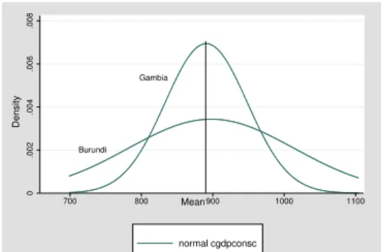
Using data, a direct illustration of Proposition 2 consists in comparing the distri-bution of the gross domestic product per capita and the spread of the epidemic for countries with a similar average GDP. Take Gambia and Burundi. Their average income over the period 1980-2001 is about 895 dollars, but the distribution of their
GDP is different. For Gambia, the distribution is concentrated around the mean value while in Burundi the variance is much higher as depicted in Fig 1. At the same time, the epidemic in the two countries follow distinct patterns. In Gambia, the spread of the epidemic is slow, the average prevalence over the period 1980-2001 is 1.12% while its peak reached 2.27% of the adult population infected in 2000. On the other hand, the epidemic is widespread in Burundi with a prevalence level of 7.47% on average over the last two decades and with a peak reaching 10.25% in 1992. According to Proposition 2, if both countries have similar transmission rate, similar disutility from protection and similar cost of infection, the higher income risk in Burundi explains why the propagation of the epidemic was faster in Burundi than in Gambia. Burundi Gambia 0 .002 .004 .006 .008 700 800 900 1000 1100 normal cgdpconsc Density Mean Figure 1: Distribution in GDP p.c.
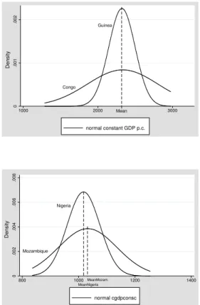
Fig. A and B, in the Appendix, depict the distributions of the GDP per capita for a couple of African countries. Comparing Congo and Guinea leads to a similar illustration of Proposition 2 in the sense that Congo has a riskier income and a more widespread epidemic than in Guinea. Similarly, Mozambique and Nigeria have an equivalent constant GDP per capita but their distributions of GDP per capita suggest that Mozambique is a much more volatile country in terms of national revenues than is Nigeria. This stylized fact must be related with the state of the epidemic. In Mozambique, the proportion of HIV-infected individuals among the adult population is twice as big as in Nigeria. In 2001, the prevalence reached 13% in Mozambique and 5.8% in Nigeria.
This brief overview supports the mechanisms outlined in the section. To properly
test our prediction, we have collected data to constitute a panel of 43 countries3 over
the period from 1980 to 2001. The countries are all the countries in Sub-Saharan Africa except for the small countries for which HIV prevalence is not reported by UNAIDS.
3
Dataset and Econometric Issues
3.1
Measurement of macroeconomic instability
Testing Proposition 2 requires to find out an appropriate measure of income un-certainty in order to test whether it is a significant predictor of HIV prevalence controlling for income. We choose the Real Business Cycle methodology to estimate the macroeconomic instability of the African economies and more precisely, we apply the Hodrick Prescott filter to extract the cyclical component of the Gross Domestic Product per capita. Hodrick and Prescott (1981) allows to generate the non linear trend of the series. This trend stands for a weighted average of the past, current and future values of the series and the difference between the actual value of the variable and the trend is the cyclical component. This measure of the cyclical component is a good indicator of the annual shocks for several reasons. First, it is detrended in the sense that it is independent of the mean of the series under consideration. For each country, the mean of the cyclical component over the period is null. Second, taking into account the previous and future values of the series it avoids the drawback of the standard coefficient of variation that considers only two periods and often leads to spurious growth rate.
−400 −200 0 200 400 shocks in constant GDP p.c. 1980 1985 1990 1995 2000 years
Côte d’Ivoire Mali Zimbabwe
Figure 2: Cyclical Component in GDP p.c. 39 or 40 countries.
Fig. 2 displays the annual fluctuations in per capita GDP for Cˆote d’Ivoire, Mali and Zimbabwe. It illustrates the phenomenon for countries where the HIV/AIDS epidemic exhibits different patterns. Two noteworthy differences are Mali and Zim-babwe. While Mali has one of the slowest HIV propagation in Africa, Zimbabwe is hard-hit by the epidemic with a prevalence reaching 33.7% of the adult population in 2001. As far as their respective economic instability, the graph clearly shows that in Zimbabwe the fluctuations in GDP per capita are greater and much more frequent than in Mali. Over the period 1980-2001, Zimbabwe experienced frequent
nega-tive shocks of large magnitude. Cˆote d’Ivoire illustrates an intermediate situation
concerning both HIV dynamics and income volatility.
As in Hodrick and Prescott (1981), the standard deviation of the cyclical
compo-nent is used as an index for the variability of the series Xit and we get the following
variable: stdshockXi = " 1 22 t=22 X t=1 (Xit− HP trendit)2 #1/2 (3) The database covering 22 years, we benefit from a sufficiently long length of time to get a consistent measure of the macroeconomic instability for each country of the sample. The standard deviation of the annual deviations from the trend should be viewed as a characteristic of the national economic volatility over time. The stan-dard deviation of the shocks in GDP for each country of the sample is summarized in Table 1a. A first look at the data suggests that the countries which exhibit the highest variances are also those with the highest levels of HIV prevalence. At the top of these variances in GDP, are Botswana, Namibia, Swaziland and Zimbabwe which are also the worst-affected countries. At the other extreme, Benin, Mada-gascar, Mali, Niger and Senegal exhibit slightly volatile GDP per capita, given that in Madagascar the epidemic is not yet generalized and that Senegal is known as a success story in preventing the epidemic from spreading (Putzel 2006).
3.2
Econometric Model
We aim to figure out whether the agents incorporate the income instability in their decision making about investing in self-protection. Since we have national data rather than individual data, we test whether countries with highly unstable economy
exhibit higher levels of HIV prevalence than those with stable economy and we study whether decomposing the income series keeps positive and significant the relation between GDP and HIV prevalence. Formally, we test whether the growth in prevalence is increasing with economic instability.
The rate of HIV prevalence is predicted using UNAIDS data despite the contro-versy saying that their prevalence levels are overestimated compared to the levels found in the Demographic and Health Surveys for two reasons. First, the panel di-mension of UNAIDS data brings more information and more variability than do any cross sections and it enables us to control for individual unobserved heterogeneity. Second, even if the overestimation was true, the prevalence levels would be overes-timated in the same way for each country of our sample so that the comparability across countries and across time prevails even after adjustment.
We estimate the HIV prevalence through a dynamic specification for two reasons. First, since the level of prevalence at date t is a function of the stock of HIV-infected agents who were contaminated before date t (i.e. the prevalence in t − 1) and of the flow of newly contaminated agents, it is straightforward to describe the prevalence as a state dependent phenomenon. Second, the prevalence rate reflects an aggregation of the individual behaviors in the extent to which the more numerous are the agents who have undertaken risky sexual behaviors in a given year, the higher the growth in HIV prevalence during that year since UNAIDS provides the rate of prevalence at the end of the year. The economic models on the rational epidemic of HIV/AIDS show that the agents decide on whether to protect taking into account the probability of becoming infected from a unprotected sexual intercourse and this probability depends directly on the level of prevalence in the previous period.
Note that a close look at the evolution of the epidemic over time suggests non-linearities in the prevalence. The epidemic goes on increasing in most countries in Sub-Saharan Africa over the first fifteen years of the epidemic and after reaching a peak of HIV prevalence, the rate of growth diminishes. To incorporate this non-linearity and given that the epidemic is said to be generalized as soon as the rate of national HIV prevalence exceeds 1% (UNAIDS 2006), the model will incorporate the number of years since the epidemic became generalized in the country. The dynamic specification detailed below does not enable us to introduce a quadratic term for the lagged prevalence.
3.3
Estimation strategy
The standard dynamic model is written:yit = αi+ ρyit−1+ Xit0 β + γt + εit, ∀i, ∀t (4)
where yit is the dependent variable, yit−1 its lag, Xit the set of covariates
in-cluding the constant, αi the individual-specific effect, t the time trend and εit the
disturbances. We choose the System-Generalized Method of Moments specification to estimate (4) because the dynamic panel bias makes the estimation by Ordinary Least Squares inefficient. The dynamic panel bias results from the correlation be-tween the fixed effect and the lagged dependent variable. Hence we need to eliminate
the αis. Difference-GMM or System-GMM are two alternatives depending on the
transformation made on the equation. Taking the first differences of equation (4), we obtain:
∆yit = ρ∆yit−1+ ∆Xit0β + γ∆t + ∆εit, ∀i, ∀t (5)
where ∆yit = yit−yit−1. In equation (5), the correlation between ∆yit−1and ∆εit
requires the use of instrumental variables. In a panel data setting, the time series dimension offers the lagged values of the regressors as potential candidates for the
instruments. Anderson and Hsiao (1982) propose to use ∆yit−2 or yit−2 as
instru-ments for ∆yit−1 and to estimate the model by the instrumental variable method.
Later, regarding the low efficiency of the Anderson Hsiao estimates, Arellano and Bond (1992) propose to estimate the model by the Generalized Method of Moments rather than the IV technique, to extend the set of instrumental variables to the entire past values and took into account the heteroskedasticity and autocorrelations of the perturbations. This technique is called the difference-GMM. The limitations of this approach are substantial. One limitation is the loss of information due to the first differentiation of the equation. Another is that the first differenced GMM estimator suffers from downward bias and low precision, especially when the value of the autoregressive coefficient ρ increases toward unity (Blundell and Bond 1998).
The alternative approach consists in using both the equations in levels and in first differences in a system of equations. The advantages of the system-GMM encompass the increase in precision and sample size, the ability of identifying the time-invariant regressors, and that it behaves better than the difference GMM for models where
the autoregressive coefficient is high (Blundell et al 2000; Roodman 2006). The dynamic model to be estimated is written as follows.
HIVit= αi+ ρHIVit−1+ β0Iit+ β1IRit+ Cit0 β2+ γt + εit (6)
where HIVit is the HIV prevalence, HIVit−1 its lag, Iit the proxy for national
income, IRit the measure of income risk, Cit the set of control variables including
the constant, αi the country specific effect, t the time effect and εitthe disturbances.
Specifying the econometric model in a dynamic framework allows us to predict the change in prevalence or the gross incidence rate by controlling for the lagged prevalence. It does not deal with the net incidence rate because we do not observe the HIV-infected agents who leave the stock. The set of control variables includes the urbanization rate, the literacy rate, religious indexes and the number of years since the epidemic became generalized (see table 1b for data definition and sources). The role of the covariates is to determine, for any given level of previous prevalence level, what induces some levels of risk taking and hence, a more or less rapid prop-agation of HIV in the population.
3.4
Some Tests
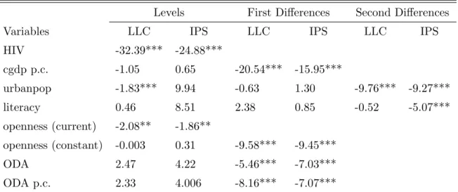
First-of-all, before estimating the econometric model, panel unit root tests are ap-plied to avoid spurious regressions related to the presence of non stationary variables in the left- or right-hand side of the equation. To examine the stationarity properties of the time-varying variables, we apply Levin et al (2002) and Im et al (2003) panel unit root tests. More details on these procedures and the results of the tests are displayed in Table 1c in the appendix. When a variable is found to be integrated of order 1 and 2, we introduce it respectively in first and second differences in the estimations.
In a system-GMM specification, consistent estimates require valid instruments and homoskedastic and uncorrelated errors. We check for the validity of the instru-ments through the Hansen test of overidentifying restrictions. Hansen test is used to ensure the absence of correlation between the instruments and the disturbances
of the model (Sevestre 2002). We correct for possible heteroskedasticity in the error terms and test for the autocorrelation of order 1 and 2 in the errors in first differences through the Arellano-Bond test.
Given the literature on the effects of the epidemic on the productivity, GDP and growth in African countries, we are particularly cautious with the potential endogeneity bias. Accordingly, we check for the endogeneity of the variable GDP per capita through the Hausman test. Formally each econometric model is estimated twice. One estimation considers GDP per capita as exogenous and the other one as endogenous and both estimations are compared in the test to know which one is consistent. When the Hausman test is rejected, we use instruments to overcome the simultaneity between income and HIV prevalence as suggested in Sevestre (2002). In the appendix, estimation outputs will report the statistic of the test.
Lastly, to ensure that the shocks in GDP per capita and in yields are exogenous, we check whether the HIV prevalence Granger causes these fluctuations. Table 1d displays the results from the tests. Results suggest that the rate of prevalence does not Granger cause the contemporaneous shocks in yields and in GDP. This rules out the possibility that the spread of AIDS are driving the large macroeconomic fluctu-ations that one country may experience. Concerning the gross domestic product, it helps in predicting the prevalence while the prevalence does not provide information to predict GDP per capita. In addition, when regressing the cyclical components on the prevalence and the estimated death rate due to AIDS, these regressors does not appear statistically significant.
4
Empirical Evidence
4.1
Naive estimations: HIV prevalence and GDP
The objective of this subsection is to check whether our database provides a positive relationship between income and the HIV/AIDS epidemic in Africa, as found in previous works. The naive estimation consists in testing whether a growth in income per capita is associated with a growth in prevalence.
Since the variable gross domestic product per capita was found to be integrated of order 1, we can not introduce it in levels but in first differences. Formally, we
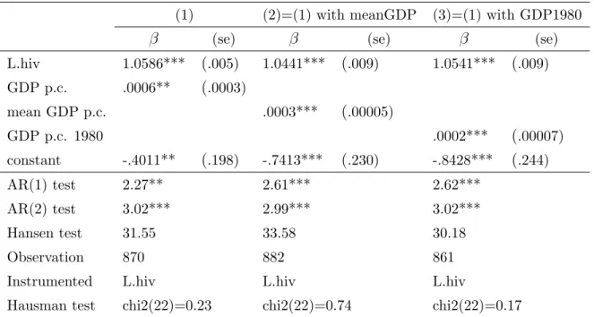
do not study the effect of the level of income but rather the effect of the growth in GDP or the level of enrichment of the country on HIV prevalence. Starting with the GDP per capita in first differences, it is found that an increase in the gross domestic product per capita leads to a rise in the prevalence rate given the previous state of the epidemic (see column 1 in Table 2). The more prosperous the country becomes, the more affected it is by the HIV/AIDS epidemic.
As a robustness check, the next step consists in verifying whether the relation still holds when using the indicator of national income in level. Since the GDP per capita is not stationary, proxies are required (see column 2 and 3 in Table 2). The effect of the level of GDP at the beginning of the period and that of the mean of the GDP per capita over 1980-2001 are estimated. Whatever the proxy used, it is found out that richer countries exhibit a higher growth in prevalence. It was worth making use of these proxies to ensure that the relation is robust, but for the rest of the empirical work, the variable GDP per capita, even in first differences, is favored because dealing with panel data, this time varying variable provides more information about the countries’ standards of living.
Our database confirms previous findings and the following two subsections are devoted to the empirical test of Proposition 2. Note that a particular attention is paid to the effect of the income on prevalence. To overcome the puzzle detailed in sections 1 and 2, we should find that introducing the cyclical component of GDP in standard deviation makes the positive relation between GDP and prevalence disappear.
4.2
Prevalence, GDP and GDP instability: A test of our
prediction
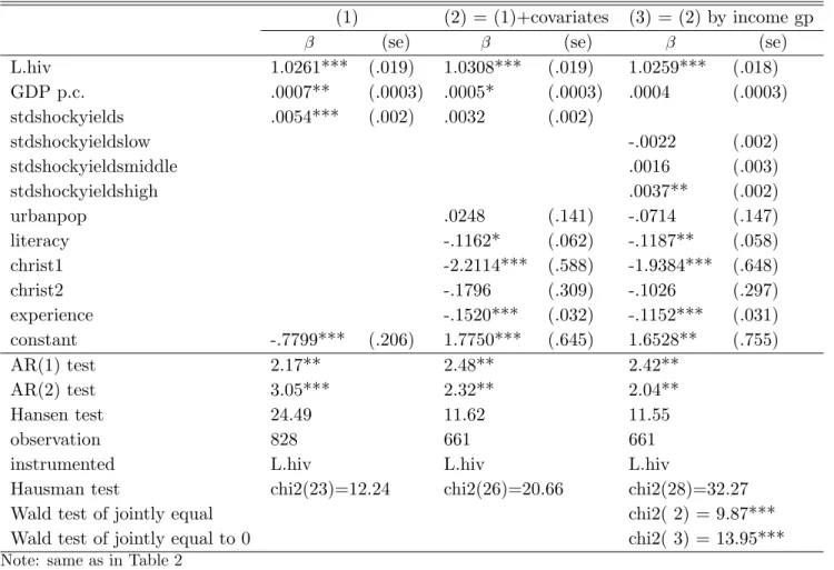
Our prediction is supported by the data when introducing the standard deviations of the cyclical component of the GDP per capita. Table 3 displays the benchmark estimation results from estimating equation (6). The estimations suggest that the volatility in per capita GDP influences the dynamics of the HIV/AIDS epidemic in Sub-Saharan Africa. More volatile economies have larger growth in HIV prevalence with other characteristics held constant. As highlighted by the theoretical model proposed in Section 2, the microeconomic foundations behind this macroeconometric result is that people living in countries that are historically volatile and prone to
great and frequent fluctuations in national income have less incentives to take care of their health status and to invest in self-protection. In fact, whether they are infected or not, the individuals are not convinced that their living conditions will be improved in the future, on the contrary, the likelihood of frequent variations in their living standards is dramatically high. We found that everything held constant, on average, one standard deviation increase in the income instability leads to an increase in prevalence of 0.35% per year.
Extracting the deviations from the trend shows that the variance plays a role in explaining the growth in prevalence and that the GDP per capita is not a good predictor for prevalence anymore. The decomposition of the series enables us to state that the average level of income is not sufficient and taken alone may lead to spurious and counter-intuitive results since it encompasses both the trend and the fluctuation of the series.
To go deeper in analyzing the relationship between macroeconomic volatility and HIV prevalence, we investigate whether the effect depends on the income level. The objective is to figure out whether rich countries are more vulnerable to economic shocks or in other words, whether people living in rich countries are more likely to engage in risky behaviors when facing fluctuating income than do people in poorer countries or the reverse. We classify our observations by income group such that the low-income group encompasses countries from the first quantile of per capita GDP, the middle-income group countries from the second quantile and the high-income group countries from the highest quantile. To test for heterogeneous effects, we interact these three dummy variables with income volatility in the baseline dynamic model.
Applying a Wald test to know whether the coefficients are jointly equal to zero suggests that the effect of macroeconomic instability on prevalence is statistically significant (see column 4 of Table 3). As found above, the pooled effect of income risk is statistically different from zero, meaning that macroeconomic instability has a broad impact on the path of the epidemic. A second Wald test is applied in order to test whether the coefficients associated with each income group are equal, the result is that the impact of economic instability on the HIV prevalence does not vary by income group. However, the results suggest that the impact is not significant for low- and middle-income countries while it is positive and statistically
significant for the high-income group. Richer countries are found to be more sensitive
to macroeconomic uncertainty than their counterparts. These results provide a
possible explanation for the fact that in Sub-Saharan Africa, rich countries are the most severely hit by the HIV/AIDS epidemic. It is suggested that the individuals in rich countries are more vulnerable to fluctuations in revenue. One might argue that instability turns out to have a significant effect on the prevalence in rich countries because fluctuations are potentially larger there than in low- and middle-income countries. But, we used Hodrick Prescott filter to get fluctuations that are detrended to avoid this possibility. The non linear trend reflects the evolution of the income series over time for each country and the fluctuations are the deviations from this trend. Moreover the standard deviation of the fluctuations encapsulates both their frequency and their size and there is no reason why rich countries should exhibit more frequent fluctuations than their counterparts.
In rich countries, one standard deviation increase in income risk leads to a rise of prevalence of 0.34% per year on average and with other explanatory variables held constant. In this estimation, GDP per capita is devoid of its predictive power and the puzzle is lifted as expected. In brief, this analysis by income group shows that the widespread levels of infection in rich African countries are probably due to their vulnerability to economic instability rather than to their level of economic development as such. However this result is no more true when correcting for the endogeneity of the GDP per capita.
4.3
Some remarks on the control variables
The persistence of the Epidemic The persistence of the epidemic in each
coun-try is captured by the variable called experience which turns out to be significantly and negatively associated with HIV prevalence in all regressions. It means that the more persistent the epidemic in the country, the slower is the growth in prevalence. Two interpretations of this result are proposed. First, this finding validates one of our theoretical predictions stating that the risk taking of HIV-infection is negatively related to the proportion of infected agents in the population. Here we found that the duration of the epidemic influences its growth as if people fear to become infected as the epidemic is spreading. Second, a complementary interpretation is that the longer the period of time since the epidemic became generalized, the more informed people are. Once generalized, the existence of AIDS is hardly denied since it takes
part of everyday life for most inhabitants who probably know someone who was or is infected. If the epidemic is generalized during a long period of time, collective information induces safer practices that in turn, slower its growth.
Literacy and urban population The interplay between the literacy rate and the
prevalence is found to be statistically significant and negative. The spread of the HIV/AIDS epidemic is slower in countries where the literacy rate is high, suggesting that sensitization campaigns are more efficient when addressed to educated people as shown in de Walque (2007). One additional interpretation, in line with the bottom line of the paper, is that educated people hold potentially good jobs and have more to lose if they become infected. In that sense, they are willing to invest more in self-protection.
As mentioned in the theoretical section, the rate of urbanization could be consid-ered as a proxy for the access to health care facilities. The rate of urbanization was included as a control variable to capture the fact that a higher urbanization may potentially induce a lower cost of self-protection given that living in urban areas offers a larger access to sensitization campaigns and a wider condom availability. However, the rate of urban population appears to have no influence on the spread of the epidemic.
Religion and prevalence We found that religion takes a part in explaining HIV
prevalence. By dividing the countries into three groups according to their level of Christianity, the estimations suggest that highly evangelized countries have a higher probability of exhibiting a widespread epidemic than do less evangelized countries. More precisely, the highly evangelized countries are more affected than the countries where over half of the population is evangelized but where church members are less than 60% of the population and even more affected than the countries with less than 50% of evangelized people. Interpreting the result on religious affiliations is twofold. On one hand, Christian people may be more affected by the HIV/AIDS epidemic because women are more emancipated than in Muslim societies (the age of first sex is lower, the number of lifetime sexual partners is higher). On the other hand, polygyny is more extended in Muslim societies than in Christian societies even though in Sub-Saharan Africa polygyny is not only related to religious aspects. But, if the percentage of polygamous marriages is higher among the Muslims than
among the Christians, this would explain why they are less severely affected by the epidemic than the Christians since polygyny is associated with a lower number of occasional sexual partners and extramarital sexual intercourses, and hence to a lower risk of HIV-infection.
5
Robustness checks and Extensions
5.1
Robustness checks
We proceed to some robustness checks to see whether the coefficient of the volatility in GDP remains stable and significant after introducing additional regressors in the benchmark equation. The objective is to rule out the possibility that other mechanisms drive the significant and positive relation between income risk and the spread of the epidemic.
The first two columns of Table 4 test whether the coefficient on the volatility in GDP remains stable and significant when controlling for trade openness. The idea behind this inclusion of openness relies on two literatures and aims to eliminate the possibility that openness acts as a third variable which could be at the origin of both the expansion of the epidemic and income volatility. Indeed, on one hand, Oster (2008) suggests that the levels of exports are positively driving the HIV in-cidence in Africa due to its resulting rise in mobility and on the other hand, trade openness is known to induce external risk. Openness is likely to enhance national macroeconomic instability and at the same time, is likely to rise the prevalence such that the positive relationship between volatility and HIV may appear only due to the omission of the variable openness. We test this possibility with two measures of openness. Columns 1 and 2 estimate the contemporaneous effects of openness on prevalence by introducing, respectively, openness in current terms and openness in constant terms in first differences since the latter turns out to be a process integrated of order 1. Our estimation results claim that the relation between HIV prevalence and income instability is not a spurious relation that would have emerged from the omission of the variable openness. Whatever the measure of openness included in the regression, the association between the spread of the epidemic and GDP volatil-ity is still positive and significant and GDP per capita is still devoid of its predictive power. Note that the contemporaneous degree of openness does not influence the
HIV prevalence.
Column 3 checks for the possibility that experiencing armed conflict increases income volatility that in turn boosts the spread of the HIV/AIDS epidemic. We introduce a dummy for armed conflict as control variable because a country prone to armed conflicts is likely to be much more volatile than a peaceful country. The dummy variable is equal to 1 if the country is experiencing an armed conflict in the given period of time and 0 otherwise. We do not distinguish according to the duration of the conflict. What matters is that the country is currently in conflict leading to two consequences. On one hand, the conflict might make the economy of the country sluggish, leading to a fall in the income level and a rise in the in-come volatility. On the other hand, the bleak prospects due to being in conflict might induce people to engage more likely in risky sexual behaviors. If this scenario was validated by the data, we would get that income instability is not significant anymore and that the likelihood of experiencing an armed conflict is positively and significantly associated to HIV prevalence. Actually, this scenario is not validated by the data. Conflicts are not driving the relation of interest between income risk and the epidemic. Income risk is still a good predictor of HIV prevalence and armed conflict appear negatively related to the spread of the epidemic in the country. Pos-sible explanations for this negative contemporaneous association between conflict and prevalence are that the conflict kills especially the agents who were already infected (military and agents who engage in the battle because their infection makes them have less to lose) and that the conflict reduces the mobility and the possibility to have unsafe sex.
We argued that the macroeconomic volatility influences the spread of the epi-demic through a fall in the incentives to engage in self-protection. Another chan-nel through which the positive association between prevalence and macroeconomic volatility might have occurred is through the aid flows. Accordingly, more stable countries are likely to receive a larger amount of aid flows compared to unstable countries and these aid flows might be targeted or used by the local government to fight the epidemic. If such a scenario prevails, then stable economies are less affected by the epidemic thanks to the aid received and the unstable nations are more affected by AIDS not due to the income risk as such but due to its induced lack of resources. To rule out this possibility, we introduce the contemporaneous amount of official development assistance and aid as control variable. Column 4
and 5 in Table 4 show that the instability in GDP p.c. remains significantly and positively related to HIV prevalence even after introducing the total aid flows and the aid flows per capita respectively. Aid flows are found to be exogenous in our specifications. This suggests that the amount of aid is not allocated in response to the HIV/AIDS epidemic. Only the amount of total aid flows is found significant even if its effect is very low.
As a general comment on the robustness checks, note that the regression coef-ficients for the variable of interest are quite similar across equations 1-5 since one standard deviation increase in income risk induces an annual rise of the prevalence ranging from 0.37 to 0.44% on average, with other characteristics held constant.
5.2
Extension: Instability in agricultural yields
The role of crop shocks is explored as an extension of the model to see whether the relation remains valid when another economic risk is considered. We investigated the role of instability in the gross domestic product to insert our contribution in the existing literature on national income and prevalence, but one might wonder whether the volatility in gross domestic product is the most appropriate proxy for the volatility in individual wealth. GDP is an indicator of standards of living and gives some worthwhile information about the potential public investment. However in most African countries, the majority of the population is working on the fields while agriculture is not productive and hence, stands for a thin part of the GDP. For instance, in Zambia, on average 75% of the population is working in agriculture
while the share of the agricultural sector in GDP is only 19%. The remaining
81% come from other sources and their profits do not benefit directly to the wide majority of the population. Farmers have access to these resources only through public spending if they are used to finance social programs but do not constitute individual wealth as such. This example is representative of the situation in most countries within Sub-Saharan Africa. In this context, investigating the role of the volatility in agricultural yields provides some additional insights into the relationship
between economic instability and the spread of the epidemic. The volatility in
agricultural yields over the previous two decades is proxied by the standard deviation of its cyclical component (see Tables 1a and 1b).
the volatility in yields as the independent variable of interest. The evidence shows a positive association between the variance of the fluctuations in yields and the prevalence in most estimations. Countries in which the yields are highly volatile are much more affected by the epidemic than their counterparts. High and frequent crop shocks discourage people to invest in self-protective behaviors all the more than in most countries, the vast majority of the population is working in the agricultural sector, have no outside option to avoid crop shocks and their livelihoods are directly affected by these fluctuations in yields. In columns 1 and 2, GDP per capita is still significantly and positively related to the prevalence. Contrary to previous estimations, the effects of GDP per capita is not offset by the effects of the economic volatility because here the volatility in yields is used instead of its own volatility. However in Column 1, the standardized regression coefficient for volatility in yields exceeds that for the income meaning that a standard deviation-change in yields instability has a greater impact on prevalence than a standard deviation-change in GDP growth. An increase in one standard deviation in yields instability and in GDP growth lead to a rise of 0.46% and 0.15% of the prevalence respectively. To get the same change in prevalence as the change resulting from a one-standard deviation change in yields instability, the growth in GDP per capita must increase by three standard deviations.
Column 3 in Table 5 studies the heterogeneous effects of the volatility in yields according to the income group. The coefficient on volatility in yields is not identi-cal for the three income groups, as confirmed by the Wald test. The relationship between volatility in agricultural yields and the spread of the epidemic exists only for the high-income group. These results suggest that the richest countries are more vulnerable to crop shocks in the sense that their population reacts more by engaging in risky behaviors when experiencing frequent fluctuations in agricultural yields than do the agents living in low and middle-income countries. These findings confirm the prediction that controlling for income, the higher the instability in crop revenues, the steeper is the growth in prevalence. Unlike the pooled regressions, GDP per capita turns out to be not significant.
6
Conclusion
To our knowledge, this analysis is the first attempt to link the incentives to adopt risky sexual behaviors through the spread of the HIV/AIDS epidemic with the eco-nomic instability. To establish this link, we built a simple theoretical model and tested it using a panel of African countries.
The present study reaches three conclusions. First, the average level of income is insufficient in predicting prevalence in the region. When introducing measure of instability in GDP, GDP per capita is devoid of predictive power and the puzzle of the positive relationship between national income and prevalence in Africa is lifted. Second, our findings suggest that the instability in gross domestic product per capita and in yields influence the spread of the epidemic. More volatile economies reach higher levels of HIV prevalence. Third, the interactions between macroeconomic instability and prevalence were investigated by income group and in some cases, it is shown that rich countries are more vulnerable to economic volatility than their counterparts. This suggests that the high prevalence in the rich African countries is due to their economic instability, instead of the level of economic development as such.
We think that the impact of income instability on the incentives for self-protection is the major and most appropriate channel through which instability affects the HIV prevalence. The argument behind is that experiencing frequent and large fluctua-tions in national income and in yields reduces the opportunity cost of infection, makes people consider the risk of HIV-infection as a minor risk and hence leads to a rise in the incentives to adopt risky sexual behaviors. In the paper, alternative channels (trade openness, conflict and aid flows) are explored and are rejected by the data.
The limitations of this study are mainly due to the dataset. We used macroe-conomic data while microemacroe-conomic data would have been more appealing to di-rectly predict the individual behaviors toward the risk of infection. Nevertheless self-reporting about sexual practices induces large measurement errors and misre-porting, and, as far as we know, no database mixing sexual behaviors and time series of revenue is available. In a macroeconomic setting, we are not able to control for a wide range of variables because of multicollinearity issues.
The paper is based on the central hypothesis that nowadays, HIV-infection is a matter of choice and incentives. Of course, not all African people have perfect knowledge about the risk of HIV-contamination, about how to use condom properly and some individuals, particularly women, have no power to negotiate on sexuality issues. However previous studies show that even well-informed agents are engaging deliberately in risky sexual attitudes. As a policy implication, the conclusions of the paper promote the protection of the agents against income shocks and public spending to provide them good and stable living conditions as a way to enhance their incentives to invest in self-protection and take care of their health status in Sub-Saharan Africa.
In this paper, we examined the particular case of individual decision about self-protection against HIV/AIDS but the bottom line may apply to other investments in health care. In particular, it is possible to derive and test the same framework for individual’s or household’s decision to use mosquito nets, to filter water or to opt for vaccination in Africa. In these cases also, the agents do not massively opt for self-protection even though the cost of self-protection is low and the agents are informed about the health risks.
References
[1] Alvarez, C., Li, V., Zanakis, S.H., 2007. Socio-Economic Determinants of HIV/AIDS Pandemic and National Efficiencies. European Journal of Opera-tional Research 176, 1811-38.
[2] Anderson, T.W., Hsiao C., 1982. Formulation and Estimation of Dynamic Mod-els Using Panel Data. Journal of Econometrics 18, 47-82.
[3] Arellano, M., Bond, S., 1991. Some Tests of Specification for Panel Data: Monte Carlo Evidence and an Application to Employment Equations. Review of Eco-nomic Studies 58 (2), 277-97.
[4] Bloom, D.E., Mahal, A., Sevilla, J., and River Path Associates. 2001. AIDS and Economics. Paper prepared for Working Group 1 of the WHO Commission on Macroeconomics and Health 2001.
[5] Blundell, R., Bond, S., 1998. Initial Conditions and Moment Restrictions in Dynamic Panel Data Models. Journal of Econometrics 87, 115-43.
[6] Blundell, R., Bond, S., Windmeijer, F., 2000. Estimation in Dynamic Panel Data Models: Improving on the Performance of the Standard GMM Estima-tor. In: Baltagi B.H. (Eds), Nonstationary Panels, Panel Cointegration and Dynamic Panels, Advances in Econometrics, vol 15. p. 53-91.
[7] Bonnel, R., 2000. Economic Analysis of HIV/AIDS. ADF 2000 Background Paper, World Bank.
[8] Centre for Study of Civil War. Armed Conflicts 1946-2003. Uppsala University. http://www.prio.no/CSCW/Datasets/Armed-Conflict/.
[9] Clark, C.R, Vencatachellum, D., 2003. Economic Development and HIV/AIDS Prevalence. Scientific Series CIRANO.
[10] de Walque, D., 2006. Who gets AIDS and how? The Determinants of HIV Infection and Sexual Behaviors in Burkina Faso, Cameroon, Ghana, Kenya and Tanzania. Policy Research Working Paper 3844, Washington, DC, World Bank.
[11] de Walque, D., 2007. How Does the Impact of an HIV/AIDS Information Cam-paign Vary with Educational Attainment? Evidence from Rural Uganda. Jour-nal of Development Economics 84, 686-714.
[12] Eeckhoudt, L., Godfroid, P., Marchand, M., 1998. Risque de Sant´e, M´edecine
Pr´eventive et M´edecine Curative. Revue d’Economie Politique 108 (3), 321-37.
[13] Geoffard, P.Y., Philipson, T., 1996. Rational Epidemics and Their Public Con-trol. International Economic Review 37 (3), 603-624.
[14] Heston, A., Summers, R., Aten, B., 2006. Penn World Table Version 6.2. Cen-ter for InCen-ternational Comparisons of Production, Income and Prices at the University of Pennsylvania. September 2006.
[15] Hodrick, R.J., Prescott E.C., 1981. Post-War U.S. Business Cycles: An Empir-ical Investigation. Northwestern University, Center for MathematEmpir-ical Studies in Economics and Management Science, Discussion Papers 451.
[16] Im, K.S., Pesaran, M.H, Shin, Y., 2003. Testing for Unit Roots in Heterogeneous Panels. Journal of Econometrics 115, 53-74.
[17] Kazianga, H., 2004. HIV/AIDS Prevalence and the Demand for Safe Sexual Behavior: Evidence from West Africa. Unpublished, Columbia University. [18] Lachaud, J.P., 2007. HIV prevalence and poverty in Africa: Micro- and
maco-econometric evidences applied to Burkina Faso. Journal of Health Economics 26, 483-504.
[19] Levin, A., Lin, C.F., Chu, C.S.J., 2002. Unit Root Test in Panel Data: Asymp-totics and Finite Sample Properties. Journal of Econometrics 108, 1-24.
[20] Luke, N., 2006. Exchange and Condom Use in Informal Sexual Relationships in Urban Kenya. Economic Development and Cultural Change 54 (March), 319-348.
[21] Oster, E., 2005. Sexually Transmitted Infections, Sexual Behavior and the HIV/AIDS Epidemic. Quarterly Journal of Economics 120 (2), 467-515. [22] Oster, E., 2008. Routes of Infection: Exports and HIV Incidence in Sub-Saharan
[23] Philipson, T., 2000. Economic Epidemiology and Infectious Diseases. In: Cu-lyer A.J., Newhouse J.P. (Eds), Handbook of Health Economics, vol 1. North Holland, Amsterdam. p. 1762-99.
[24] Philipson, T., Posner, R.A., 1993. Private Choices and Public Health: The AIDS Epidemic in an Economic Perspective. Harvard University Press.
[25] Putzel, J., 2006. Histoire d’une Action d’Etat: La Lutte Contre le Sida
en Ouganda et au S´en´egal. In : Philippe Denis and Charles Becker (Eds),
L’Epid´emie du Sida en Afrique Subsaharienne: Regards Historiens. Editions
Karthala. p. 245-70.
[26] Roodman, D., 2006. How to Do xtabond2: An Introduction to ’difference’ and ’System’ GMM using Stata. Working Paper 103, Center for Global Develop-ment.
[27] Rothschild, M., Stiglitz, J.E.,1970. Increasing Risk: 1. A Definition. Journal of Economic Theory 2, 225-43.
[28] Sevestre, P., 2002. Econom´etrie des Donn´ees de Panel. Dunod.
[29] UNAIDS, 2004. Report on the Global AIDS Epidemic 2004.
[30] UNAIDS, 2006. Report on the Global AIDS Epidemic 2006. p. 8-50. [31] UNAIDS, 2007. AIDS Epidemic Update 2007.
[32] Viscusi, W.K., Evans, W.N, 1990. Utility Functions that depend on Health Status: Estimates and Economic Implications. The American Economic Review 80(3), 353-74.
Figure A and B: Income distribution for a couple of comparison countries Congo Guinea Mean 0 .001 .002 1000 2000 3000 normal constant GDP p.c. Density Graphs by country Mozambique Nigeria MeanMozam. MeanNigeria 0 .002 .004 .006 .008 800 1000 1200 1400 normal cgdpconsc Density Graphs by country
Table 1a: National measure of the instability in constant GDP per capita and in agricultural yields
Countries StdshockGDP Stdshockyields Countries StdshockGD Stdshockyields
Angola - 58.459 Liberia 67.746 53.342 Benin 22.325 48.044 Madagascar 17.744 40.898 Bostwana 170.993 43.807 Malawi 29.636 213.421 Burkinafaso 20.456 64.735 Mali 33.323 98.273 Burundi 40.973 40.199 Mauritania 30.201 75.738 Cameroon 83.228 87.021 Mozambique 51.812 75.474 Central Africa 33.932 75.681 Namibia 174.567 82.870
Chad 32.141 73.9216 Niger 37.579 47.577
Congo 199.016 64.675 Nigeria 29.880 100.507 Cˆote d’Ivoire 71.190 74.381 Rwanda 79.871 104.219
RDC 43.497 11.797 Senegal 45.297 79.229
Djibouti 253.008 104.014 Sierraleone 41.220 65.857
Equ. Guinea 321.186 - Somalia 44.184
-Eritrea 27.573 212.697 South Africa 94.870 390.427 Ethiopia 24.630 99.006 Sudan 32.786 99.065 Gabon 315.335 91.558 Swaziland 133.303 276.695
Gambia 22.006 71.968 Togo 34.035 65.378
Ghana 36.035 81.816 Uganda 23.267 127.235
Guinea 46.949 37.291 Tanzania 38.900 125.639 Guinea Bissau 59.000 87.911 Zambia 39.097 312.449 Kenya 21.703 162.859 Zimbabwe 195.204 368.227 Lesotho 35.691 140.779