Simulating Targeted Policies with Macro Impacts: Poverty Alleviation Policies in Madagascar

(1)

D

OCUMENT DE

T

RAVAIL

DT/2004/11

Poverty Alleviation Policies in Madagascar:

a Micro-Macro Simulation Model

Denis COGNEAU

(2)

POVERTY ALLEVIATION POLICIES IN MADAGASCAR: A MICRO-MACRO SIMULATION MODEL

Denis Cogneau DIAL - UR CIPRÉ de l’IRD

cogneau@dial.prd.fr

Anne-Sophie Robilliard DIAL - UR CIPRÉ de l’IRD

robilliard@dial.prd.fr

Document de travail DIAL / Unité de Recherche CIPRÉ

Novembre 2004

ABSTRACT

We present the framework of a macro-micro simulation model for the study of the impact of economic policies on income distribution and monetary poverty in Madagascar. Modelling options and choices are discussed for the micro-economic module and for the macro-micro linkages. Econometric estimations and calibration of the occupational choice / labor income part of the micro-economic module are presented and commented. Some illustrative simulations of poverty alleviation schemes are also implemented and analyzed.

Keywords: Economic Modelling, Micro-Simulation, Income distribution, Poverty Reduction, Dual

Labor Markets, Occupational Choice, Madagascar

RÉSUMÉ

Nous présentons le cadre d’un modèle de simulation macro-micro pour l’étude de l’impact des politiques économiques sur la distribution du revenu et la pauvreté monétaire à Madagascar. Les options et les choix de modélisation sont discutés pour le module micro-économique et pour les liaisons micro-macro. Les estimations économétriques et la calibration du modèle de « choix » d’occupation et de revenu du travail sont présentées et commentées. Des simulations illustratives de stratégies de réduction de la pauvreté sont aussi mises en œuvre et analysées.

Mots-clefs: Modélisation économique, micro-simulation, distribution du revenu, réduction de la

pauvreté, choix d’occupation, dualisme du marché du travail, Madagascar

(3)

List of tables

Table 1 : Agricultural profit function ... 31

Table 2 : Occupational choice / Labor income model parameters after micro-calibration... 32

Table 3 : Aggregated social accounting matrix... 33

Table 4 : Minimum yearly wages, 1990-96 ... 33

Table 5 : Distribution of beneficiary households across quintiles ... 33

Table 6 : Macroeconomic impact of alternative policies ... 34

Table 7 : Employment impact of alternative policies ... 34

(4)

1 Introduction

1

This chapter aims at presenting a modelling technique integrating a static (CGE type) macro module with a static micro-simulation module of labor sup-ply/income and consumption demand based on cross-section survey data. This simulation model, thereafter designated as the micro-macro model, is dedicated to simulate the short-medium term impact of economic shocks and policies on income distribution and monetary poverty. It is applied to the case of Mada-gascar. The micro-simulation module is built upon a structural micro-economic model of occupational choices and labor income. It is estimated on a standard cross-section micro-economic dataset deriving from a ”multitopic household sur-vey” (see Scott, 2003).

Section 2 presents the options oﬀered by current econometric practice and the modelling choices that have been made for this work. Section 3 presents the micro-simulation module and its econometric estimation. Section 4 presents the integration procedure with the macro-module and simulations.

2 Motivations for an integrated micro-macro model

Most common macro models used to analyze distributional issues are able to take into account some structural features of the economy and general equilib-rium effects as well as the functioning of factor markets, but they usually rely on the definition of representative household groups characterized by different combinations of factor endowments and possibly different behaviors. The het-erogeneity of the population of households is thus integrated in a scarce and unsatisfactory way since the inequality modeled is essentially the inequality between the representative groups. In many situations, the decomposition of observed inequality evolution has shown that within-group inequality changes are very often as important as between-group changes. This explains why tra-ditional macro-economic models may appear unsatisfactory in dealing with dis-tributional issues. Different approaches that rely on full household/individual samples have been developed recently to overcome this difficulty. They differ

1_{We thank the National Institute of Statistics of Madagascar for providing the data. Special}

thanks to Mireille Razafindrakoto, François Roubaud and members of the MADIO project in Antananarivo for fruitful discusssions about our research and the Malagasy economy. We also thank François Bourguignon, Jesko Hentschel, Philippe Leite, Dominique van der Mensbrug-ghe, Luiz Pereira da Silva and Abdelkhalek Touhami for discussions about previous versions of the present work. The usual disclaimer applies.

(5)

in how they account for micro-behaviors and in the degree of integration of the macro and micro ”stories”. Several approaches can be distinguished and are put in comparison in the present volume (see also Cogneau, Grimm, Robilliard 2003).

The ”integrated micro-macro” approach presented here attempts to fully integrate household income generation modeling within a multi-market frame-work with endogenous commodity prices and factor returns. It also allows the simulation of structural policies that select individuals within the intra-group

distribution. This kind of simulation is, by construction, made diﬃcult by

the representative groups assumption of standard macro economic models. In comparison with the ”top-down” approach, the integrated approach puts more weight on the micro-economic side of the model; as a consequence, its macro-economic and multi-market framework is also less sophisticated.

2.1 Benefiting from advances in economics and

micro-econometrics

The first motivation for building an ”integrated micro-macro” model is to take full advantage of the theoretical and technical advances in micro-economics and micro-econometrics of the modeling of complex micro-behaviors within specific market structures.

The ”integrated micro-macro model” starts with a structural modelling of occupational choices and labor income formation. It may also include a micro-model of consumption choices. In the language of econometrics, ”structural” means that the micro-behavior of agents is explicitly modeled as the result of an optimization program taking macro variables as given, such as returns to categories of labor, product prices or the unemployment risk. In the context of micro-macro models, micro-structural modelling of household and individual decisions draws on the large literature related to labor and consumption micro-economics and micro-econometrics. This allows the consideration of complex production, labor supply and consumption behaviors of heterogenous house-holds and individuals confronted with transaction costs, information asymme-tries, employment rationing, that is various kinds of ”market imperfections”. For instance, Cogneau and Robilliard (2001) take into account the non-recursive behavior of Malagasy agricultural households in the absence of a market for agri-cultural labor which prevents the equalization of the productivity of agriagri-cultural labor between households. Structural micro-econometric estimation also takes

(6)

explicitly into account the market structure which constrains the agents’ de-cisions. For instance Cogneau (1999 and 2001) estimates a labor income and occupational choice model for the city of Antananarivo under various assump-tions on the segmentation (dualism) of the urban labor market, drawing from Magnac (1991). The remaining micro-parameters which can not be identified in micro-econometric estimations, due to lack of information or other identifi-cation problems, are ”calibrated” for the simulation, in line with the spirit of calibrated CGE macro-models. For instance, in both cited cases, heterogenous preferences for consumption decisions are calibrated on available survey data; some parameters related to labor supply like the variance of reservation wages are also calibrated.

2.2 Preserving the consistency between micro and macro

variables

The second motivation for building an ”integrated micro-macro” model is to preserve full consistency between the specification of micro-behaviors and the specification of macro aggregates. This may be desired on pure epistemological grounds : this is the ”aggregation issue”. But it may also be desired for welfare analysis purposes: this in turn is what we might call ”interlinked welfare issues”. Micro-economic behavior can be made consistent with a multi-sector and multi-agents macro-economic framework through a number of calibration tech-niques that will be described thereafter. A fully consistent integration of micro-behaviors into a macro framework is not straightforward, and never completely achieved. It is however theoretically permitted by the structural nature of the specifications: agents react to prices and other signals which are determined at the macro-level. It is a fact that even simple micro-economic structural mod-els do not lead to perfect aggregation: the ”response function” of an average of agents does not look like the behavior of an individual agent, and most of the time has no analytical expression. This absence of a strong aggregation property prevents from separating the macro and the micro part if one wants to preserve mathematical consistency. As a result, in order to reach a consistent micro-macro equilibrium, micro-decisions have rather to be summed up and confronted with each other and with other macro-aggregates. At the end of the algorithmic resolution of the model, all aggregates coming from the households’ micro-part, like the supply of categories of labor, the consumption demand, or total wage earnings must be equal to the corresponding macro-aggregates like

(7)

the demand for categories of labor, the domestic supply of consumption goods, and the wage bill.

It is well known that the structural micro-economic modeling of labor sup-ply and occupational choices (not to mention consumption demand behavior in some contexts) raises issues such as the heterogeneity of reservation wages, the indivisibility of hours worked or the rationing of labor supply in dualistic labor market. Discrete and/or constrained choices are the rule, between inactivity and work, between part-time jobs and full-time jobs, or between sectors or oc-cupations. In this context, the envelope theorem no longer holds for computing equivalent welfare variations: one can not derive marginal welfare changes from observed choices and prices variations, even when price variations are small enough. Moreover, micro-agents welfare components are usually interlinked. One of the most simple examples of this is the structural relation that exists be-tween the wage level and the utility of leisure: agents decide whether to accept a wage offer by comparing it with a ”reservation wage”. Another example is the link between wage offers and non-monetary utility of jobs: agents compare two wage offers on the basis of their heterogenous preferences for the jobs (com-pensating differentials story), or discount from each wage some cost of entry

in the corresponding occupation (segmentation story).2 _{If such phenomenons}

prevail, (i) wage earnings do not adequately reflect welfare levels, and (ii) some combinations of wages and occupational choices are not compatible. Therefore, separating income issues from occupational choice or labor supply issues at the micro-level, like in reduced form models, may lead to misrepresent not only the welfare distribution but also the income distribution.

2.3 Simulating targeted policies with macro impacts

Even if it can be more justified on methodological grounds, structural mod-elling usually precludes a high level of disaggregation of market segments and/or sectors, because of intrinsic econometric and algorithmic diﬃculties on which we shall give more detail hereafter. As a result, the integrated approach is less suited for the study of subtle intersectoral reallocations of supply and de-mand and fine modifications of the price and earnings schedule. Besides, a full structural model of household behavior, including production, labor supply, consumption, schooling and migration decisions, can not be econometrically

es-2_{A third example coming from another field is the interlinkage of consumption and}

(8)

timated, even if it were theoretically available. One has to focus on the most relevant behavioral features for the policy question under review or else resort to ”piecemeal modelling” following Orcutt’s strand of micro-simulation analy-sis (Orcutt, 1976). This means that a multi-purpose model is relatively out of reach with this approach. An ”integrated micro-macro model” is relatively more suited to exploring general poverty reduction strategies and demo-economic is-sues on the one hand, and micro-structural and targeted policies on the other hand.

The study of medium-term general poverty reduction strategies may require a lower level of disaggregation than the study of macro-structural policies like trade policies. For instance, trade-oﬀs between a ”rural stance” (productiv-ity enhancing rural investments) or an ”urban stance” (job creation in towns) in poverty reduction strategies may be usefully studied like in Cogneau and Robilliard (2001) within a dual economy model with two or three sectors (agri-culture, informal, formal) which endogenize the labor allocation of households,

consumption demand, and, if possible, migration decisions.3 _{Demo-economic}

issues may also be studied by integrating a structural income micro-simulation module to a stochastic micro-demographic projection module, in the spirit of the micro-simulation models designed in developed countries to study the re-form of pension systems. For instance, the distributional impact over fifteen years of the AIDS epidemics has been studied that way by Cogneau and Grimm (2002), as well as the long-term impact of education policies by Grimm (2003 and 2004), both in the case of Côte d’Ivoire. It should however be kept in mind that in such frameworks, dynamic investment decisions remain exogenous and call for other methods to be properly analyzed (see Townsend and Heckman contributions in this volume).

Aside from this kind of general statistically-grounded experiments, simulat-ing short-term targeted policies with macro-impacts might be the true compara-tive advantage of the ”integrated micro-macro” approach. This is the road that is explored in this contribution. By targeted policies we mean policies whose aim is to reach specific categories of the population, most usually among the poor, through various targeting devices. They include labor market interventions like wage policies, workfare programs or job creation linked to foreign direct invest-ment, but also land reforms and product markets interventions like marketing boards. One first problem is to evaluate the eﬃciency of the targeting device.

(9)

When the targeting is imperfect and depends on self-selection of individuals, a micro-structural model may be most useful. For instance, how many people will choose the new wage oﬀer from a workfare program or a from an export processing zone? Another problem is to assess the overall distributional impact of such policies within and outside the target population, when their magnitude is big enough to have a macro-economic impact. Here then, a micro-macro clo-sure may help. For instance, how many people will benefit from an increase in the minimum wage, how will this increase be transmitted to other segments in the labor market through a raise in the informal labor earnings; or what are the respective impacts of a job creation policy and of a wage policy in a developing

country urban labor market?4 How much a food price subsidy operated through

a marketing board will benefit to small farmers and how much will it benefit to the urban poor through a relative food price reduction? How much of the workforce a workfare program will attract and what will be the consequence on the production and prices of other sectors and hence on the overall income distribution? The empirical illustrations chosen in this paper try to address this type of questions.

3 A micro-simulation module

3.1 The main labor income model

The labor income model draws from the spirit of Roy’s model (1951), as formal-ized by Heckman and Sedlacek (1985), which is pointed out by Neal and Rosen

(1998) as the most convincing model for explaining labor income distribution.5

At each period, each individual pertain to a given family or household whose composition and location is exogenously determined.

If he/she is more than fifteen, he/she faces three kinds of work opportunities: (i) family work, (ii) self-employed work, (ii) wage work.

Family work includes all kinds of activities under the supervision of the household head or the spouse, that is family help in agricultural or informal activities, but also domestic work, non-market labor and various forms of de-clared ”inactivity”. In farming households, the farm head is considered as a

4_{Cogneau (1999 and 2001) shows that a micro-macro model of the distribution of income is}

able to simulate the historical decrease in poverty observed in the city of Antananarivo during the 1995-99 period, thanks to job creation and minimum wage increases in the formal sector.

5_{See also Magnac (1991) and Cogneau (2001) in the case of urban labor markets in}

(10)

self-employed worker bound to the available land or cattle whose farming occu-pation never changes (although he may work part-time in another occuoccu-pation, see extension below). Self-employed work corresponds to informal independent activities. Wage work includes all other kinds of workers, mainly civil servants and large firm workers.

3.1.1 Potential individual earnings outside of the household

To self-employed work (j = 1) and wage-work (j = 2) we associate two potential

earnings functions. Individual potential earnings wji are seen as the product

of a ”task price” πj (j = 1, 2) with a fixed idiosyncratic amount of eﬃcient

labor which depends on observable characteristics Xi (education, labor market

experience and geographical dummies) and on unobservable skills tji:

ln w1i = ln π1+ Xiβ1+ t1i (1)

ln w2i = ln π2+ Xiβ2+ t2i (2)

Returns to characteristics β_j are diﬀerentiated by sector and by sex.

3.1.2 Reservation wage in non-farm households

To family work we associate an unobserved individual value that also depends on household characteristics, and on other members’ labor decisions, gathered in a Z0vector:

lnw_e0i= (X0i, Z0h) β0+ t0i (3)

For non-agricultural households members, w_e0 may be seen as a pure

reser-vation wage. X0 contains the same variables as X (education, labor market

experience and geographical dummies), plus a variable indicating the link to the household head (head/spouse/child/other), and the father’s occupation for

the head. Z0includes the demographic structure of the household. In order to

account for collective hierarchical decisions and for an income eﬀect on partic-ipation to the labor market, it also includes, in the case of non-head members, the head’s occupational choices and earnings, and, in the case of non-spouse secondary members, the spouse occupational choice and earnings. Finally, it includes the household’s non-labor income.

(11)

3.1.3 Farm income and reservation wage in farm households

To farming households we associate a reduced farm profit function derived from a Cobb-Douglas technology with homogenous labor:

ln Π0h= ln p0+ α ln Lh+ Zhθ + u0h (4)

We assume that the farm head always work on the farm. As a result, only non head members may choose whether to participate in farm work. Moreover,

e

w0 is assumed to depend on the individual’s contribution to farm profits. We

evaluate this contribution while holding fixed other members decisions and the farm global factor productivity u0:

ln ∆Π0i= ln p0+ ln¡Lαh+i− Lαh−i

¢

+ Zhθ + u0h (5)

where Lh+i = Lh, Lh−i= Lh− 1 if i is actually working on the farm in h,

and Lh+i= Lh+ 1, Lh−i= Lh alternatively.

Here again the labor decision model is hierarchical between the household head and non-head members, and simultaneous among non-head members: in making his/her decision, each non head member does not take into account the consequences of it on other secondary members. In the case of agricultural households, we then write the family work value as follows:

lnw_e0i= (X0i, Z0h) β0+ γ. ln ∆Π0i+ t0i (6)

where γ stands for the (non-unitary) elasticity of the value of family work in agricultural households to the price of agricultural products. In this case,

X0 includes the same variables as X (education, labor market experience and

geographical dummies), plus a variable indicating the link to the household head

(spouse/child/other), while Z0includes the household’s demographic structure,

non-labor income, and, should this happen, the (part time) occupation of the farm head .

3.1.4 Occupational choice

Finally, comparing the respective values attributed to the three labor opportuni-ties, workers allocate their labor force according to their individual comparative

(12)

advantage:6

i chooses family work iﬀw_e0i> w1i andwe0i> w2i

i chooses self-employment iﬀ w1i>we0i and w1i> w2i (7)

i chooses wage-work iﬀ w2i>we0i and w2i > w1i

3.1.5 Labor market

These selection rules complete the theoretical occupational choice / labor income model on the supply side. For each segment of the labor market, one may define the set of individuals who supply labor on this segment:

Sj= {i / wji= max(we0i, w1i, w2i)} (8)

Theoretically speaking, if one wants to keep in line with the Mincerian equa-tions (1) and (2), labor supply in the wage-sector and in the self employment sector should be expressed in eﬃciency units of labor, that is:

Ls₁= P i∈S1 w1i π1 and Ls₂= P i∈S2 w2i π2 (9) In the family work sector or in agriculture, since labor is not diﬀerentiated, the number of workers equals the quantity of labor.

Ls₀=P_{1 {i ∈ S}0} = Card (S0) (10)

In the case of the family-work/agriculture sector and in the case of the self-employment sector, there is no labor market. Households or individuals either

consume their own production or sell it on goods markets. Prices p0and π1are

then determined on the goods market equilibrium.

In the wage-work/formal labor market, one has to add aggregate demand for labor functions in order to fully describe the labor market in the competitive case:

6_{We introduce here the supplementary assumption that individuals compare}

self-employment and wage-work opportunities only in terms of earnings. In other words, these two work opportunities do not bring diﬀerential non-monetary benefits. This assumption is relaxed in the segmented model presented thereafter, which is the one that is empirically implemented.

(13)

Ld₂= L2(π2/q2 −

)Q2 (11)

where q₂ stands for the price of other inputs and where Q2 is aggregate

demand for good 2 (or production in sector 2).7

3.1.6 A pluri-activity extension8

We wish to allow individuals to pursue outside part-time activities when they work for the family. We first have to introduce a ”part-time” variable in the wages and benefits equations to take into account the variability of hours worked:

ln w1i = ln π1+ X1iβ1+ δ1.Ti+ t1i (12)

ln w2i = ln π2+ X2iβ2+ δ2.Ti+ t2i (13)

with δ1< 0, and δ2< 0. We may then redefine ”full time” incomes:

lnw_b1i= ln w1i− δ1.Ti

lnw_b2i= ln w2i− δ2.Ti

We finally simply assume that when reservation value is close enough to either ”full-time” wage or self-employment benefits, individuals choose to work (simultaneously or successively) inside and outside the family. The listing of selection rules then becomes:

i chooses full time family work iﬀw_e0i> (1 + a) .wb1i andwe0i> (1 + a) .wb2i

i chooses family work and self-employment iﬀ (1 + a).w_b1i>we0i> (1 − a). bw1i andwb1i>wb2i

i chooses family work and wage-work iﬀ (1 + a).w_b1i>we0i> (1 − a). bw1i andwb2i>wb1i

i chooses full time self-employment iﬀ (1 − a). bw1i>we0i andwb1i>wb2i

i chooses full time wage-work iﬀ (1 − a). bw2i>we0i andwb2i>wb1i

The workfare program that is simulated thereafter introduces a new kind of

7_{This demand for labor function could only be estimated using a time series of}

cross-sections, like in Heckman and Sedlacek (1985). In the empirical implementation, we shall-however keep the total formal employment fixed as a matter of simplicity, even though it is at the expense of theoretical consistency.

(14)

part-time job oﬀer which is paid at a rate w3. In this case, once the former

selection rule has been run, we add the following rules:

if i had chosen full-time family work i takes the workfare oﬀer iﬀ 2 × w3> (1 − a) . ew0i

if i had chosen self-employment i takes the workfare oﬀer iﬀ w3+ w1i>wb1i

if i had chosen wage-work i takes the workfare oﬀer iﬀ w3+ w2i>wb2i

3.1.7 A segmented labor market extension

Suppose now that the labor market is segmented. This means that the selection conditions (7) do not hold in many observed cases: some individuals would prefer to work in a given segment but could not find any available job opportunity. In practice, we restrict the rationing of jobs to the wage-sector. Then, without

loss of generality,9 _{we may introduce a segmentation variable:}

lnw_e2i= lneπ2+ X2iβe2+ η2i (14)

And modify the selection rules as follows:

i is observed in family work iﬀ w_e0i> w1i andwe0i >

w2i

e w2i

i is observed in self-employment iﬀ w1i>we0i and w1i>

w2i

e w2i

(15)

i is observed in wage-work iﬀ w2i e w2i >w_e0i and w2i e w2i > w1i

The segmented labor market extension may be combined with the part-time extension (and actually is, in the empirical implementation).

The occupational choice / labor income may then be estimated by maximum likelihood like before. The segmented model contains the previous competitive model as a particular constrained case (Magnac, 1991).

Since the segmented model has more degrees of freedom than the competitive model, more parameters have to be calibrated.

With π2 given exogenously by wage setting rules (minimum wage moves,

price indexation, and Philips curve for instance), a decrease (resp. an increase)

9_{The reservation value}_w_e

0 then includes the cost of entry into the informal activities. See

(15)

of_eπ2may then simulate hirings (resp. lay-oﬀs) in the wage sector.

3.2 Results of estimation and of calibration

The micro-simulation module is based on a household sample provided by the EPM (Enquête Permanente auprès des Ménages) survey for the year 1993/94, and simulates income generation mechanisms for approximately 4,500 house-holds. We use both the pluri-activity and the segmented labor market exten-sions for the estimated micro-simulation model. Econometric and calibration details are provided in the Appendix.10

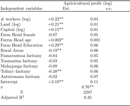
Table 1 shows the agricultural profits function, associated to the farm heads in agricultural households.

[ Insert Table 1 here ]

The number of family workers comes out with a coeﬃcient that is consistent with usual orders of magnitude: a doubling of the work force leads to an around 20% increase in agricultural profits. The amount of arable land and of capital also come out with a decreasing marginal productivity and a similar impact on profits (a doubling making a 20% increase again for land, and a 15% increase for capital). Age and education of the farm head also come out as significant.

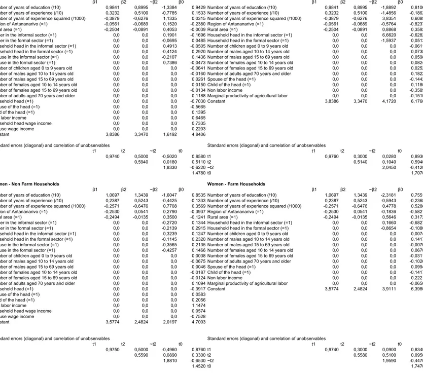
Table 2 shows the partly estimated and partly calibrated ³β₁, β₂, eβ₂, β₀´ sets of parameters for the four categories of the labor supply model, and the calibrated variance-covariance matrix of¡t1, t2,et2, t0¢.

For men, the returns to education are rather close in the informal and wage-sectors. For women, they are higher than for men and higher in the formal sector. Returns to labor market experience (or to job tenure) are higher in the wage-sector for both sexes and similar for men and women. Informal benefits are 25% lower in the rural areas, and 25% lower for women in the Antananarivo region (faritany) than in other faritany. Costs of entry in the wage-sector vary negatively with education and experience, are, not surprisingly, 20 to 25% higher in the rural areas and higher for women in the Antanarivo faritany. A house-hold head working in the wage-sector leads other members of the househouse-hold to do the same, which again is reflected in a lower cost of entry. The reservation wage (value of inactivity) in non-farm households is positively related to educa-tion, the eﬀect of which lies in-between the returns to education in the informal

1 0_{Detailed results from econometric estimation before calibration are available from the}

(16)

sector and the ”discounted” returns (monetary returns less cost of entry) in the wage-sector. Participation to the labor market is higher in both the rural area and the Antananarivo faritany (lower reservation wage). Almost by definition, heads are less often inactive and non-labor income increases the propensity to stay inactive. The demographic structure of the household and the hierarchical decisions of other members play only a minor role in the decision to participate. In farm households, educated people strictly prefer to work outside the farm, whether in informal or wage jobs. When the farm head already works part of his time in non-agricultural activities, other members tend to do the same. Activity is more diversified out of agriculture in the Antananarivo faritany. The estimate of the effect of the marginal productivity of labor has a negative effect on the farm-work value. This effect uncovers the fact that in resource-endowed agri-cultural households, with more land or more capital and hence a higher labor productivity, agents are more prone (have more opportunities) to diversify their activities. It should however be stressed that this diversification of activity is not frequent among agricultural households. Only 13% of the total agricultural households labor force works outside the farm at least part-time, the bulk of which (10%) working in part-time informal activities. Diversification is higher for household heads (20% work outside of the farm) than for other members (10% only work outside). This absence of real opportunities for diversification of activities among agricultural households, especially the poorest, is one of the most important features of the distribution of income in Madagascar, and strongly constrains the short-run impact of agricultural price and workfare poli-cies that are examined in the remainder of this paper. This feature also explains why we could not obtain an acceptable estimate for the elasticity (γ, see above) of the farm-work choice to the agricultural price. In the remainder, we calibrate this elasticity to one, like in other sectors.

4 Macro-micro model characteristics and

simu-lation

Once calibration has been achieved, the segmented occupational choice and labor income model is ready for simulation. With the price of the formal good p2

taken as the numeraire, the relative prices, p0/p2and π1/p2, and the cost of entry

index for the wage-sector,_eπ2/p2, are determined by the general equilibrium on

(17)

individuals to the aggregate demand for each task derived from consumption choices and production processes, as explained hereafter.

4.1 The micro part

Starting from the micro-model of occupational choice and labor income pre-sented in section 3.1, we detail how a simple and consistent general equilibrium model may be written, drawing from Cogneau (2001) and Cogneau and Robil-liard (2001).

At the micro-level and on the supply side, complementary intermediate in-puts are determined from idiosyncratic technical coeﬃcients and added to real

benefits to obtain the agricultural production of each household Q0h. The

re-sulting agricultural production is then split between the production sold in ex-port markets and the production sold in domestic markets (or consumed inside the household), through a standard constant (and homogenous) elasticity of transformation function, with an idiosyncratic export orientation parameter cal-ibrated from micro-data on agricultural production. This makes the composite

agricultural producer price idiosyncratic (p0h), depending on each household’s

specific technical coeﬃcients and export orientation, on the exogenous agricul-tural export price pe₀and on the domestic price pd

0 and on other input prices.

Self-employed informal production and producer price p1are computed the

same way, starting from w1i/π1 and adding intermediary inputs. Informal

pro-duction consists in non-tradable trade activities and services that are sold to households.

In formal production, capital use is complementary to the quantity of ef-ficient labor Ls

2 =

P

i∈S2

w2i

π2. A fraction of capital income is distributed to resi-dent households using the survey information on declared dividends: households declaring dividends are awarded a fixed share of total dividends from formal capital.

Household income is then equal to the sum of agricultural benefits (in farm households), self-employment benefits and wage earnings, non-labor income stemming from capital income, and transfers.

In the demand side, consumption choices are assumed separable from la-bor supply decisions. Idiosyncratic saving rates and idiosyncratic parameters of preference of an expenditure system with three goods (agricultural, infor-mal, formal) are calibrated from micro-data on household expenditures. Con-sumption is then split between imported and domestically produced goods by

(18)

calibrating a standard aggregate Armington CES function.11

Other components of demand for agricultural and informal products coming from the macro-part of the model add up with households’ consumption demand. Once all these elements are gathered, a general equilibrium determination of prices pd

0/p2 and p1/p2is completely defined. In the wage-sector, π2/p2is fixed

or exogenously determined, and_eπ2/p2varies to adjust the supply of wage-labor

to the exogenously determined (in the macro-part) demand for wage-labor.12

The macro-part of the model is the part that determines all other supply and demand components other than (i) the supply for labor, agricultural goods and informal goods, and (ii) the demand for consumption from households.

4.2 The macro part

The macro-part of the model corresponds to a CGE framework. Markets for goods, factors, and foreign exchange are assumed to respond to changing de-mand and supply conditions, which in turn are aﬀected by government policies, the external environment, and other exogenous influences. The model is Wal-rasian in that it determines only relative prices, and other endogenous real variables in the economy. Sectoral product prices, factor prices, and the real exchange rate are defined relatively to the formal price of goods p2, which serves

as the numeraire. The exchange rate represents the relative price of tradable goods vis-a-vis non traded goods (in units of domestic currency per unit of foreign currency).

As already said, domestic prices of agricultural (pd0) and informal (pd1)

com-modities are flexible, varying to clear markets in a competitive setting where individual suppliers and demanders are price-takers. Then, by Walras’ law, the equilibrium of the formal goods market is automatically achieved. Following Armington, the model assumes imperfect substitutability, for the agricultural and the formal goods, between the domestic commodity and imports. What is demanded is a composite good, which is a CES aggregation of imports and domestically produced goods. For export commodities, the allocation of domes-tic output between exports and domesdomes-tic sales is determined on the assumption that domestic producers maximize profits subject to imperfect transformability

1 1_{In contrast with exportable agricultural production, survey information does not give this}

split at the household level, which unfortunately precludes the calibration of idiosyncratic import shares. For simulations on the distributional impact of trade or exchange rate policies, the impact of this lack of information should be studied in more detail.

1 2_{In all simulation exercises presented thereafter, total formal employment is fixed and}

e π2/p2

(19)

between these two alternatives (at the household level, see micro-part above). The composite production good is a CET (constant-elasticity-of-transformation) aggregation of sectoral exports and domestically consumed products.

Equilibrium is defined by a set of constraints that need to be satisfied by the economic system but are not considered directly in the decisions of micro agents. Aside from the supply-demand balances in product and factor markets, three macroeconomic balances are specified in our model: (i) the fiscal balance, with government savings equal to the diﬀerence between government revenue and spending; (ii) the savings-investment balance; and (iii) the external trade balance (in goods and non-factor services), which implicitly equates the supply and demand for foreign exchange - flows, not stocks since the model has no assets or asset markets. The chosen macro closures are: (i) endogenous govern-ment savings; (ii) endogenous foreign savings; (iii) savings-driven investgovern-ment. As a result, a decrease (resp. increase) in government income translates into a decrease (resp. increase) in government savings, which in turn leads to a de-crease (resp. inde-crease) in total investment (investment is driven by savings in all experiments).

4.3 Scenarios and simulations

The model represents the behavior of a sample of 4,500 households, represen-tative of the Malagasy population in 1993/94, corresponding to a sample of 12,800 individuals aged 15 years and older, in an economy with three sectors (agricultural, formal and informal) and three goods. In order to achieve a cer-tain consistency with previous CGE exercises, household statistical weights were recomputed to comply with the income structure of a Social Accounting Matrix (SAM) for the year 1995. Order aggregates were taken from the same source (see Table 3). The reweighting procedure relies on a cross-entropy estimation (Robilliard and Robinson, 2003).

We present exploratory simulations with the objective of improving the

in-comes of the poor.13 _{In this paper we explore three alternative simulations to}

achieve this objective: a direct output subsidy on agricultural prices, a work-fare program, and an untargeted transfer program. These policies are compared both in terms of their macroeconomic impact and in terms of their impact on

1 3_{Previously we showed that neither a 20% devaluation, nor a four fold increase in}

agricul-tural tariﬀs could achieve a significant reduction in poverty and inequality indicators (Cogneau and Robilliard, 2003).

(20)

poverty and income distribution. All experiments are designed so that their ex post cost are equal (at formal prices).

The first simulation looks at the impact of a direct subsidy on agricultural production prices. The subsidy is set at 10% and is introduced as a negative tax on producer prices, thus creating a 10% gap between producer and consumer prices. Such a policy could be achieved by the intervention of a marketing board on agricultural goods markets, which would buy at high prices to producer and sell 10% lower to consumers.

In the second experiment, we simulate the implementation of a workfare scheme. Workfare programs, whereby participants must work to obtain benefits, have been widely used for fighting poverty, usually in times of crises due to macroeconomic or agro-climatic shocks (Ravallion, 1999). The workfare scheme we study is assumed to be highly labor intensive. The government buys at a fixed rate the services of labor in order to build or to rehabilitate roads and other infrastructures.14 _{Given the occupational choice model described in the previous}

section, the workfare scheme designed in our experiment can be summarized by two characteristics: the workfare wage level and the corresponding work load. We choose to design a part time workfare scheme whereby participating individuals are allowed to remain working in part in their original occupation. Whether individuals choose to participate in the workfare program depends on the level of the workfare wage and on their formal, informal, and reservation wages (see selection rule at the end of section 3.1.6). As mentioned earlier, the level of the workfare wage is fixed ex ante so that the ex post cost of the scheme matches the cost of the agricultural price subsidy. The resulting yearly wage is 257,625 Malagasy francs, which translates into 515,250 Malagasy francs in full time equivalent. Table 4 shows official minimum wages in different sectors from 1990 to 1996. Our database has been scaled to match structural and demographic features of the year 1995. Consequently, the meaningful figures are in the 1995 column. They show that our simulation workfare wage is relatively close to official minimum wages and represents 87% of the minimum wage in non agricultural sectors. Given this workfare wage level, a total of 908,470 workers -corresponding to 12.7% of the labor force — choose to participate in the workfare scheme.

The third and last simulation is a uniform untargeted per capita transfer

1 4_{For a historical record of this kind of programs in Madagascar, see Razafindrakoto and}

(21)

program. Again, the amount paid is computed so that the aggregate ex post cost of the program matches the cost of the previous programs. The resulting amount is 17,887 Malagasy francs per capita which adds up with household non-labor income (and has the corresponding micro-economic eﬀects of an increase in the value of inactivity in non-farm households).

All three programs share a high budgetary cost equivalent to almost 5% of GDP. They should therefore have large macro-economic impacts as well as the intended distributional micro-impacts.

4.3.1 Targeting issues

A central issue related to the poverty and income distribution impacts of all three simulations is the targeting properties of each scheme. Obviously, the uniform untargeted transfer per capita is distributed evenly across quintiles of income, but this not the case for the agricultural subsidy and workfare simulations. In order to explore this issue, Table 5 presents the distribution of individuals in beneficiary households across quintiles of per capita income for these two simulations.

Not surprisingly, the agricultural subsidy appears to have good targeting properties in terms of the distribution of beneficiary households. But this result does not hold when one considers the distribution of the program cost: while 83.9% of individuals in the first quintile are in a household which benefits from the agricultural subsidy, only 7.2% of the total program cost accrues to these, and the largest share (37.7%) accrues to the last quintile. This result is related to the fact that the price subsidy is proportional to agricultural output and thus, by construction, regressive in terms of program cost allocation.

When compared to the agricultural subsidy, the workfare scheme appears to be less progressive in terms of the distribution of individuals in beneficiary households, since they are distributed evenly across quintiles. But since the benefits accruing to households are not proportional to their incomes, the dis-tribution of the program cost is actually less regressive than in the agricultural subsidy experiment. The targeting performance of the workfare scheme is nev-ertheless disappointing as it fails to reach a large number of workers in poor households. This is explained by the fact that the reservation value (w_e0)

esti-mated and calibrated from actual data not only reflects preferences for family work but also includes a cost of entry component in outside informal activities.

(22)

Estimated parameters indicate for instance that activity is more diversified out of agriculture in households living in the Antananarivo faritany or in urban ar-eas, and also more in land-rich households. As a result, individuals from poor agricultural households dwelling in remote areas are given large reservation val-ues which reflect large costs of access to all markets, including the labor market. This cost of access prevents some agricultural workers from seizing the workfare job opportunities. In other words, since the workfare scheme fails to take these costs into account, it is implicitly targeted towards urban areas. As a result, it has a large impact on urban poverty (see next section).

4.3.2 Results

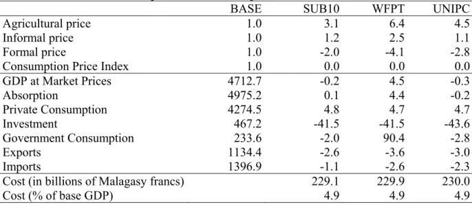
Table 6 shows various price and macro aggregate changes as a result of the three programs. Macro aggregate changes are presented in real terms.

One common point across all three experiments is the increase in the agricul-tural relative price. In particular, even the subsidy simulation leads to a 3.1% increase in the consumers’ agricultural price (relative to the consumer price in-dex). This result stems from large income eﬀects which raise the demand for agricultural products. The three transfer schemes in fact all reallocate demand out of formal goods towards agricultural goods. In all scenarios, the budgetary cost is financed by a cut in investment demand, 87% of which is demand for formal good while it is zero for the agricultural good. Given that all three sim-ulations benefit households, whose average budget share are 32%, and 57% for the agricultural and formal goods respectively, the ex ante net demands are pos-itive for the agricultural good in all three experiments. The workfare program has the strongest impact of all on the agricultural prices (6.4% increase against 3.1 and 4.5% in the other simulations) as it also leads to a decrease in the labor available for agriculture (see table 7).

Results also show that the macroeconomic impact of all three policies is dramatic in terms of investment. This result stems from the fact that the subsidy simulation has a huge budgetary cost (4.9% of GDP) which translates into an income eﬀect through the closures of both the fiscal balance and the

savings-investment balance.15 _{The GDP impact of the workfare scheme is big}

1 5_{While this cut in investment appears somewhat unrealistic and rather unsustainable in}

the long run, these closures were chosen because they appeared to be the most neutral in terms of their ex ante income distribution impact. Given the budgetary cost of the policies simulated here, any closure based on fixed government savings and investment would entail

(23)

(4.5% in real terms). The workfare program indeed corresponds to a new highly labor-intensive production of non-tradable goods (construction), which we have assumed to be entirely consumed by the government. Both the agricultural subsidy policy and the uniform transfer simulation, have small and negative GDP impacts. In the case of the uniform transfer, households are given money but they do not have to work in exchange. As mentioned earlier, all experiments were designed in order to equalize their ex post cost. As a result, all three simulations have the same impact on private consumption.

The employment impact is presented in Table 7. The top part of the table shows numbers of workers in terms of their occupational choices while the lower part presents aggregate values of the sectoral allocation of labor. Results show that the subsidy simulation leads to a mild increase in total employment. In terms of sectoral employment, labor appears to be reallocated from the informal (-6.3%) to the agricultural sector (+1.4%). As expected, the workfare scheme has a strong impact on urban under-employment with the number of inactive workers decreasing by more than 15%. It also leads to important reallocations of labor out of agricultural (-3.9%) and informal sectors (-13.3%) into workfare. As a result, the total active population increases by 3.0%. Given its design, the workfare program obviously drives transitions out of full time work and into part time work. The uniform transfer scheme has only a mild impact on the structure of employment.

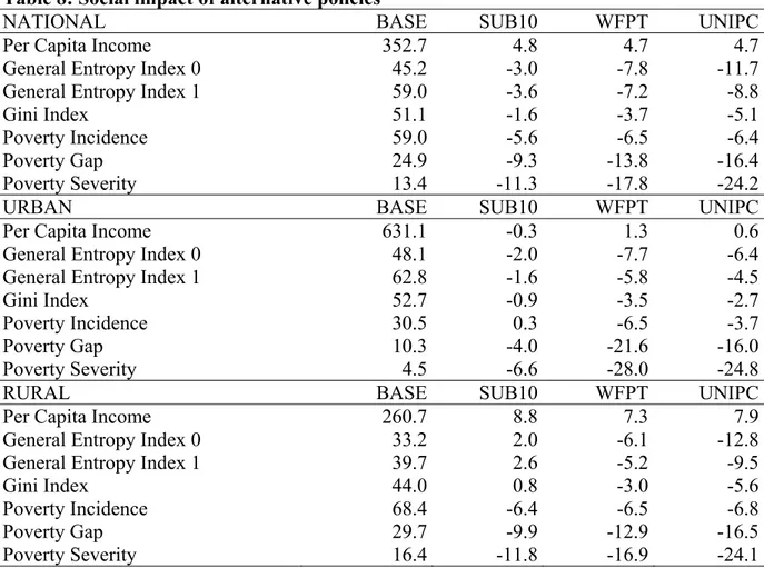
Table 8 shows results in terms of poverty and income distribution for all households, and in both urban and rural areas. Changes in three indicators of inequality are presented: the Gini index as well as two entropy indices.

All indicators show that the agricultural price subsidy simulation leads to an improvement in the distribution of income at the national level. A closer look into each area suggests that the decrease in overall inequality is mainly driven by the convergence in urban and rural per capita incomes. The introduction of a subsidy on agricultural production leaves the inequality within the rural area almost unchanged (the Gini index slightly increases by 0.8%), as well as within the urban area. As mentioned above, this absence of change in rural inequality stems from the targeting property of the subsidy whereby agricultural endogenizing either tax or saving rates, resulting in a higher ex ante impact on households’ income distribution. Another possibility would be to finance these policies using international aid.

(24)

households with higher incomes benefit more (in absolute terms) than small agricultural households. As a result, changes in poverty indicators are mainly driven by changes in per capita income.

In terms of poverty reduction, the workfare scheme has a stronger impact than the subsidy program: the poverty headcount is reduced by 6.5% while the subsidy program reduces it by 5.6%. It also has a stronger eﬀect on income dis-tribution with a 3.7% decrease in the Gini Index (compared to a 1.6% decrease with the subsidy program) and with a 17.8% decrease in the poverty severity in-dicator (compared to a 11.3% decrease with the subsidy program). This strong decrease in inequality is explained both by the convergence of average per capita incomes between urban and rural areas and by the decrease of inequality within both areas. The workfare scheme has by far the strongest impact on inequality and poverty in urban areas. Thanks to the workfare scheme, poverty incidence in urban areas decreases by more than 6%, while it remains unchanged in the case of the agricultural subsidy and is only reduced by 3.7% with the uniform transfer. Although the GDP impact of the untargeted transfer program is mild, both the poverty and income distribution impacts are significant: the program reduces the poverty headcount by 6.4% and the Gini Index by 5.1% and its impact on poverty severity is the highest among the three experiments. These results again show that the workfare scheme does not achieve much better tar-geting than the untargeted transfer program, and does not satisfactorily reach the poorest of the poor (see above).

In sum, the two targeted programs which have been examined here have indeed large impacts on monetary poverty alleviation, even once general equi-librium eﬀects are taken into account. Given the large budgetary amounts which are transferred to households, it does not come as a surprise. Apart from scaling and financing issues, the simulations however reveal that there is room for im-provements in the quality of targeting. Indeed, a general subsidy to agricultural producers does not appear to be an adequate scheme for reaching the poorest farmers as it fails in doing better than an untargeted transfer or even a work-fare scheme, even in rural areas. A general workwork-fare program oﬀering part-time job opportunities paid around the minimum wage also reaches somewhat disap-pointing results, especially in rural areas. Costs of access to the labor market prevent individuals living in remote areas and/or in poor autarkic agricultural households from seizing the workfare opportunities. The workfare scheme per-formance is relatively good in urban areas where it draws a lot of people out of inactivity or out of informal under-employment, but falls short in rural areas

(25)

where it is outperformed by the untargeted transfer.

All three schemes have been designed in order to have the same ex post budgetary cost in terms of the total amount of transfer received by households. It should however be kept in mind that they all have specific implementation costs that should be taken into account when comparing their relative eﬃciency. For instance, the implementation of an agricultural subsidy would call for the reconstruction of a marketing board which raises many institutional issues and might imply high administrative costs. Likewise, the implementation of a work-fare scheme has other costs than pure wage costs, however labor intensive it is: organizational and administrative costs, advertisement costs and input costs (see Ravallion, 1999). In this case however, we have seen that part of these additional costs are internalized by individuals who give up the workfare job oﬀers when they are too far from them. Finally, even the untargeted transfers scheme would entail an additional cost of bringing the cash to the households, even in very remote areas.

5 Conclusion

This chapter has presented the basic motivations for the construction of an inte-grated static micro-macro model for a low-income economy. It has outlined the main features of such a model in terms of micro-econometric specifications and macro-closures. Finally it has explored the use of this kind of model for the simu-lation of targeted transfer schemes dedicated to poverty alleviation. These kind of transfer schemes might be implemented either following a macro-economic shock or as permanent safety nets. For illustrative purposes, three large scale transfer schemes have been simulated and compared: (i) a price subsidy to agricultural producers, (ii) a general workfare program proposing part-time job opportunities paid around the minimum wage and (iii) a uniform unconditional and untargeted transfer provided to each individual regardless of her age and job situation. The micro-macro model gives interesting results on the counter-factual impacts of each program on the overall distribution of income, taking into account both micro-economic targeting issues and macro-economic general equilibrium eﬀects. Considerations about the financing of the programs and about their technical implementation costs could supplement the simulations in order to build realistic, eﬃcient and sustainable poverty alleviation schemes.

(26)

and disadvantages of the integrated micro-macro approach. In the first section of this chapter, we advocated the use of integrated micro-macro models on the basis of three main arguments. We first argued that the approach was well suited to incorporating current advances in the micro-econometrics of house-holds behaviors and markets structure in developing countries. The illustrations presented show the usefulness of a thorough modeling of labor supply behavior in the context of highly segmented markets. However much remains to be done to improve the modeling of agricultural households behavior whose collective production in family farms does not fit as well our ”individualistic” framework (see Cogneau and Robilliard, 2001, for an alternative). Moreover, it should be emphasized that structural estimation based on cross-sectional data may either overstate or understate the true reaction of poor households with respect to labor incentives. It would greatly benefit from the availability of dynamic panel data and/or from experimental knowledge on poor households’ responses to pro-grams (Duflo, 2003). Second, we argued that integrated tools might be desired for the sake of micro-macro consistency, as far as ”aggregation issues” and ”in-terlinked welfare issues” are concerned. It should however be stressed that such a consistency in the modeling of household welfare (labor supply, earnings, con-sumption) is obtained at the expense of sectoral disaggregation and of dynamic considerations. Depending on the policy problem at stake, trade-oﬀs must be solved inside a triangle made of ”household heterogeneity”, ”sectoral detail” and ”intertemporal issues”. We therefore argued that the static integrated tool might be better suited for analyzing the distributional aspects of general de-velopment strategies on the one hand, and for evaluating the impact of short to medium term targeted programs with macro-impacts. Through the appli-cations we implemented, we hope to have shown that integrated micro-macro modeling could be useful in the design of these latter programs. The design of other structural policies, like minimum wage increases or foreign-investment led jobs creation, could also benefit from this type of approach.

(27)

Appendix. Econometric estimation and calibration for simulation

We present here the econometric estimation and calibration of the segmented model for occupational choices and labor income.

For econometric identification, in line with our ’hierarchical-simultaneous’ model of labor decisions within the household, we must assume independence for the¡t1, t2,et2, t0¢, between individuals even among members of the same

house-hold. In the case of farm households, we also assume that u0, the idiosyncratic

total factor productivity of the household, is independent from ¡t1, t2, et2, t0

¢

for all household members16_{. We assume joint normality for the} ¡_t

1, t2, et2, t0¢

vector:

¡

t1, t2, et2, t0¢ Ã N (0,Σ) (16)

Under these assumptions, we may adopt the following estimation strategy: (i) for non-agricultural households, we estimate by maximum likelihood the occupational choice / labor income model represented by the (1)-(3) and equa-tions and the series of selection condiequa-tions (15) ; we obtain a bivariate tobit, like in Magnac (1991). We make separate estimations for each sex.

(ii) for agricultural households we follow a limited information approach: in a first step, we estimate the reduced profit function (4) then derive an estimate for the individual potential contribution to farm production (5); in a second step, estimate the reservation wage equation (3) including this latter variable as in (6),

and retaining the wage functions estimated for non-agricultural households17_.

Again, we make separate estimations for each sex, excluding the farm heads whose occupational choice is not modelled.

Maximum likelihood estimation allows for the identification of some func-tions of the coeﬃcients of wages, self-employment benefits and family work value equations. Likewise, only some elements of the underlying covariance structure between unobservables can be identified, because of the segmentation hypothe-sis and because observed wages are measured with errors and include a transient component εj (j = 1, 2) which does not enter in labor supply decisions of

(risk-neutral) individuals and which may also include the variance of hours worked.

1 6_{This latter assumption should allow for a direct identification of the ∆Π}

0 eﬀect in

e

w0,through the eﬀect of u0h. However, as ∆Π0 is presumably aﬀected by large

measure-ment errors, we exclude ’available land’ from the variables inw_e0, taking it as an instrument

for the identification of the eﬀect of ∆Π0.

1 7_{This latter option is rather inocuous for potential earnings outside the farm, as only a}

(28)

We then assume for estimation: ¡

t1, t2, et2, t0, ε1, ε2¢ Ã N (0,Σ∗) (17)

Once this posed, nine variance or correlation parameters may be identified: ρ = corr¡t1− t0, t2− et2− t0¢, σj =pvar (tj+ εj), k =

q

var(t1−et0)

q

var(t2−et2−et0) , λ1 =

corr(t1+ε1, t1−t0), λ2= corr(t2+ ε2, t2−et2−t0), µj= corr(tj+εj, t2−et2−t1)

for j = 1, 2. While all the parameters of observed earnings are identified, only the contrasts β1−β0

σ(t1−t0)and

β2−eβ2−β0

σ(t2−et2−t0)are identified. Finally, as only the reserva-tion value funcreserva-tion is distinct between members of agricultural households and members of non-agricultural households, two series of estimates are computed for β1−β0

σ(t1−t0),

β2−eβ2−β0

σ(t2−et2−t0), ρ, k, λj,whereas only one series is computed for the

pa-rameters of informal benefits and wage-earnings µ_j, β_j, σj and for part-time

parameters δj and a (see above, the pluri-activity extension).

For simulation purposes, we need to recover the parameters β₀ and eβ₂ for

e

w0 and we2 respectively, and the whole covariance structure Σ∗. We therefore

proceed to a calibration. In practice, we assume (i) that measurement errors are white noises (uncorrelated with others) and fix their variance, (ii) we fix the correlation (ρ12) between t1 and t2 and (iii) we fix the standard error of

(t2− et2− t1). We then draw for each individual a whole set of unobservables

¡

t1, t2, et2, t0, ε1, ε2

¢

, within the multidimensional normal distribution with the

covariance structure Σ∗ _{and constrain the drawings to respect the occupation}

selection rules. For instance, for an individual who is observed in the informal

sector, we start from the observed t1 + ε1 and draw all other unobservable

components conditionally on it, constraining the drawings to respect w1 >we0

and w1 > w2/we2. We finally obtain for each individual the set (we0, w1, w2,we2)

(29)

References

[1] Bourguignon F. (1990), Growth and Inequality in the Dual Model of De-velopment: The Role of Demand Factors, Review of Economic Studies, 57, 215-228.

[2] Cogneau D. (1999), La formation du revenu des ménages à Antananarivo : une microsimulation en équilibre général pour la fin du siècle, Economie de Madagascar, 4, 131-155.

[3] Cogneau D. (2001), Formation du revenu, segmentation et discrimination sur le marché du travail d’une ville en développement : Antananarivo fin de siècle, DIAL DT 2001/18.

[4] Cogneau D., A.-S. Robilliard (2001), Growth, Distribution and Poverty in Madagascar: Learning from a Microsimulation model in a General Equilib-rium Framework, DT 2001/19, 47 pp, and IFPRI-TMD Discussion Paper 61.

[5] Cogneau D., A.-S. Robilliard (2003), "Economic policies and Income Dis-tribution in Madagascar: a Micro-Macro Simulation Model", mimeo, 22 pp.

[6] Cogneau D. M. Grimm (2002), AIDS and Income Distribution in Africa: A Micro-Simulation Study for Côte d’Ivoire, Paper Prepared for the 27th Conference of the International Association for Research in Income and Wealth, Stockholm, Sweden, August 18-24.

[7] Cogneau D., M. Grimm, A.-S. Robilliard (2003), Evaluating poverty re-duction policies — the contribution of micro-simulation techniques, in Cling J.-P., M. Razafindrakoto, F. Roubaud (eds), The New International Strate-gies for Poverty Reduction, London: Routledge.

[8] Duflo E. (20003), "Scaling up and Evaluation", paper prepared for the ABCDE conference in Bangalore, 39 pp.

[9] Grimm M. (2003), "The medium and long term eﬀects of an expansion of education on poverty in Côte d’Ivoire. A microsimulation study", DIAL Working Paper DT/2002/12, DIAL, Paris.

[10] Grimm M. (2004), "A decomposition of inequality and poverty changes in the context of macroeconomic adjustment: A microsimulation study for

(30)

Côte d’Ivoire", In A.F. Shorrocks and R. van der Hoeven (eds.), Growth, In-equality and Poverty. Prospects for Pro-Poor Economic Development, Ox-ford: Oxford University Press.

[11] Heckman J., G. Sedlacek (1985), Heterogeneity, Aggregation, and Mar-ket Wages Functions : An Empirical Model of Self-Selection in the Labor Market, Journal of Political Economy, 93, 1077-1125.

[12] Magnac Th. (1991), Segmented or Competitive Labor Markets ? Econo-metrica, Vol.59, N◦_{1, pp.165-187}

[13] Neal D., Sh. Rosen (1998), Theories of the Distribution of Labor Earnings, in Atkinson A.B., F. Bourguignon (eds), Handbook of Income Distribution, North-Holland

[14] Orcutt G., S. Caldwell and R. Wertheimer (1976), Policy exploration through microanalytic simulation. Washington D.C.: Urban Institute Press. [15] Ravallion M. (1999), Appraising Workfare, The World Bank Research

Ob-server, 14(1), 31-48.

[16] Razafindrakoto M., F. Roubaud (1996), L’approche à haute intensité de main-d’oeuvre (himo): une opportunité pour Madagascar. Essai de cadrage macro-économique, Economie de Madagascar, 1, 100-129.

[17] Razafindrakoto M., F. Roubaud (1997), Une matrice de Comptabilité So-ciale pour Madagascar, Projet Madio, No. 9744/E.

[18] Robilliard, A.S., S. Robinson(2003) “Reconciling Household Surveys and National Accounts Data Using Cross-Entropy Estimation”, Review of In-come and Wealth, forthcoming.

[19] Roy A. (1951), Some Thoughts on the Distribution of Earnings, Oxford Economic Papers, 3, pp.135-146.

[20] Scott K. (2003), Generating Relevant Household-Level Data: Multitopic Household Surveys, in Bourguignon F., L. A. Pereira da Silva (eds), The Impact of Economic Policies on Poverty and Income Distribution, Evalua-tion Techniques and Tools, World Bank and Oxford University Press.

(31)

Table 1 : Agricultural profit function

Agricicultural profit (log)

Independent variables Est. s.e.

# workers (log) +0.22** 0.04

Land (log) +0.21** 0.01

Capital (log) +0.15** 0.01

Farm Head female -0.07 0.05

Farrm Head age +0.002* 0.001

Farm Head Education +0.29** 0.06

Rural Areas -0.19** 0.06 Fianarantsoa faritany -0.04 0.05 Toamasina faritany -0.03 0.05 Mahajanga faritany -0.09 0.06 Toliary faritany -0.38** 0.06 Antsiranana faritany -0.02 0.07 Intercept +3.10** 0.11 σ 0.76** N 2287 Adjusted R2 _0.35

Data Source: EPM 1993/94 survey. Field: All farming households. ** (resp. *): Significant at the 1% (resp. 10%) level.

Simulating Targeted Policies with Macro Impacts: Poverty Alleviation Policies in Madagascar

D

OCUMENT DE

T

RAVAIL

DT/2004/11

Poverty Alleviation Policies in Madagascar:

a Micro-Macro Simulation Model

Denis COGNEAU

Contents

List of tables

1

Introduction

2

Motivations for an integrated micro-macro model

2.1

Benefiting from advances in economics and

micro-econometrics

2.2

Preserving the consistency between micro and macro

variables

2.3