Science Arts & Métiers (SAM)
is an open access repository that collects the work of Arts et Métiers Institute of
Technology researchers and makes it freely available over the web where possible.
This is an author-deposited version published in: https://sam.ensam.eu Handle ID: .http://hdl.handle.net/10985/9968
To cite this version :
George CHATZIGEORGIOU, Yves CHEMISKY, Fodil MERAGHNI - Computational micro to macro transitions for shape memory alloy composites using periodic homogenization - Smart Materials and Structures - Vol. 24, n°3, p.1-17 - 2015
Any correspondence concerning this service should be sent to the repository Administrator : [email protected]
Computational micro to macro transitions
for shape memory alloy composites using
periodic homogenization
George Chatzigeorgiou
1, Yves Chemisky and Fodil Meraghni
LEM3-UMR 7239 CNRS, Arts et Métiers ParisTech Metz-Lorraine, 4 Rue Augustin Fresnel 57078 Metz, France
Abstract
In the current manuscript, a homogenization framework is proposed for periodic composites with shape memory alloy (SMA) constituents under quasi-static thermomechanical conditions. The methodology is based on the step-by-step periodic homogenization, in which the macroscopic and the microscopic problems of the composite are solved simultaneously. The implementation of the framework is examined with numerical examples on SMA composite laminates. Complexity of the composite nonlinear response and non-proportional stress state in the SMA appears, even in the case of uniaxial macroscopic boundary conditions. Moreover, under certain conditions, the composite laminate can exhibit a non-convex transformation surface.
Additionally, the transformation temperatures at various stress levels under isobaric thermal cycling can be quite different between the composite and the pure SMA.
1. Introduction
Shape memory aloys (SMAs) have been investigated for engineering applications for more than 40 years due to their ability to recover substantial deformation. The phenomen-ological modeling of the reversible martensitic transformation in SMAs has been well studied in the literature and several constitutive models have been proposed (Tanaka et al1986, Liang and Rogers 1990, Brinson 1993, Boyd and Lagou-das1996, Patoor et al 1996, Leclercq and Lexcellent 1996, Auricchio et al 1997, Anand and Gurtin 2003, Paiva et al 2005, Sadjadpour and Bhattacharya 2007, Hartl et al 2010, Chemisky et al 2011, Lagoudas et al 2012). Thorough reviews of the most common models and com-parisons between them can be found in the works of Birman (1997), Patoor et al (2006), Lagoudas et al (2006), Paiva and Savi (2006). While these materials are considered good
candidates for actuators, their relatively high cost restrains their usage in many industrial applications. Thus, alternative, less expensive solutions are investigated, including compo-sites with SMA components.
The homogenization theory of media with periodic structure is a well-established theory (Bensoussan et al1978, Sanchez-Palencia1978, Tartar1978, Allaire1992, Murat and Tartar 1997). Modeling the mechanical behavior of elasto-plastic, viscoelasto-plastic, or damaged composite materials requires advanced micromechanics and homogenization techniques from both mathematical and computational points of view (Suquet1987, Ponte-Castañeda and Suquet1997, Terada and Kikuchi2001, Desrumaux et al 2001, Meraghni et al2002, Jendli et al 2009, Mercier and Molinari 2009, Khatam and Pindera 2009, Tekoğlu and Pardoen 2010, Cavalcante et al 2011, Kruch and Chaboche 2011, Lahellec and Suquet 2013, Tsalis et al2013). Reviews of different multi-scale approaches for linear and nonlinear composites are
available in the literature (Kanouté et al 2009, Pindera et al2009, Charalambakis2010, Geers et al2010).
Recently, much research effort has focused on modeling the behavior of SMA composites. Porous SMAs have been extensively studied during the last two decades (Qidwai et al2001, Entchev and Lagoudas2002,2004, Nemat-Nasser et al2005, Panico and Brinson 2008). Moreover, in the lit-erature, certain studies on composite beams with SMA rein-forcement (Baz and Ro 1992), composite plates with SMA fibers (Rogers et al 1991, Ro and Baz 1995), and strips (Lagoudas et al1997) have been reported. Micromechanical analyses on composites with SMA reinforcement have been performed by Boyd and Lagoudas (1994), Lagoudas et al (1994), Cherkaoui et al (2000), Wang and Shen (2000), Song and Sun (2000), Marfia (2005), Collard et al (2008), Lester et al (2011) using the self-consistent and/or Mori–Tanaka methods and by Kawai et al (1999) using the method of cells. The Mori–Tanaka method has also been utilized to study SMAs with precipitates (Piotrowski et al2012). While these techniques allow us to obtain analytical or semi-analytical solutions, they can provide quite accurate results only under certain conditions: a) geometrical limitations, dealing only with matrix/ellipsoidal inclusion material systems and b) the Eshelby solution is no longer valid when the SMA is con-sidered to be the matrix of the composite. The use of periodic homogenization in SMA composites has been reported in Herzog and Jacquet (2007), but in this methodology the elastic properties of the SMA were assumed to be constant, independent of the martensite volume fraction. Indeed, the approach proposed by the authors cannot be applied when the elastic properties vary with the martensite volume fraction. In the present work, such limitation is addressed, by following a different approach based on the tangent moduli of the material constituents.
The current work introduces a computational approach for composites with SMA components, based on the periodic homogenization theory. The advantage of this approach is that it can be applied to periodic media with SMAs inde-pendent of the material constituents geometry and the choice of the SMA constitutive law. The incremental step-by-step homogenization methodology solves the problem in both the micro- and macroscale simultaneously, which is very important, especially in the cases of nonlinear materials. The computational approach is utilized in the case of composite laminates consisting of SMAs undergoing martensite-auste-nite transformation and elastic or elastoplastic materials. The obtained results show some interesting characteristics of the overall composite behavior, like non-convex transformation surfaces under certain conditions.
The organization of the paper is as follows: sections 2
and 3 present the main concepts of homogenization for nonlinear periodic media and the computational scheme based on the return mapping algorithm technique. In section4 the Lagoudas et al (2012) model, used in the numerical examples, is briefly described. The numerical studies of SMA laminate (multilayered) composites in sections5and6demonstrate the capabilities and highlights of the developed approach. Con-clusions are presented in section 7. For the completeness of
the paper, two appendices are included, which present the algorithms of the computational scheme and the semi-analy-tical solution details for the case of composite laminates.
2. Theoretical framework of homogenization
The principles of periodic homogenization have already introduced in the pioneering works of Bensoussan et al (1978), Sanchez-Palencia (1978), and for elastoplastic com-posites in Suquet (1987). Here the main points of the theory are briefly summarized.
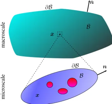
In periodic homogenization a composite is described through the introduction of two suitable scales. Thefirst scale, the microscopic, represents the microstructure considering different material constituents and their geometry. The second scale, the macroscopic, considers the overall body as an imaginary homogeneous medium (figure1). The properties of this hypothetical homogeneous medium are identified through the solution of the microscale problem.
At the macroscale, the continuum body occupies the space¯ with volume V and bounded by a surface ∂ ¯ with normal unit vector n. Each macroscopic point is assigned with a position vectorxin¯(figure1). On the other hand, at the microscale level, there is a representative volume element (RVE) that occupies the space with volume V and is bounded by a surface ∂ with normal unit vector n. Each microscopic point is assigned with a position vector x in (figure1). In the sequel, a bar above a symbol ({•}) denotes a macroscopic quantity or variable.
In the periodic homogenization framework, the two scalesx(overall scale) and x (microscale) are connected by a characteristic length ε through the relation =
ε
x x. This characteristic length needs to be very small, tending to zero (i.e., the microstructure should be extremely small compared Figure 1.Schematic presentation of composite: macro- and microscale.
to the size of the composite), for the homogenization method to be accurate. Some typical examples of materials with periodic microstructure that meet these requirements are particulate-reinforced, alignedfiber, multilayered, and woven fabric composite.
In the following subsections the main principles that govern the two scales and the correlation between them are described. It is worth mentioning that the current work deals with quasi-static processes and considers the influence of the temperature in the composite’s mechanical response. The spatial distribution of the temperature inside the material would require a fully coupled thermomechanical analysis, accounting for latent heat and thermal conduction effects, which exceeds the scope of this contribution. Thus, in all the studied numerical examples the temperature profile is con-sidered known (i.e., spatially uniform temperature conditions).
2.1. Microscale
Since each RVE represents a single point in the macroscopic body, every microscopic variable is a function of both the macroscopic position of the specific RVE, x, and the microscopic position, x.
Upon mechanical loading, it is assumed that each microscopic point undergoes a displacement u. In this paper small deformation processes are considered, thus the problem is formulated using small strain assumptions. For the kine-matics on the RVE, the usual relation between the second-order symmetric microscopic strain tensor ϵ and the dis-placement vector u are considered,
ϵ = +
[
[
]
x x u x x u x x ( , ) grad ( , ) grad ( , ) in , (1) 1 2 t⎤ ⎦where the superscript t denotes the transpose of a matrix and = ∂
∂
grad {•} {•}x . Ignoring micro-body forces and inertia effects, the micro-equilibrium is written
σ x x =0
div ( , ) in , (2)
where σ is the second-order symmetric microscopic stress tensor,div{•}=grad{•}: , and i is the second-order identityi tensor. For materials with thermomechanical response, such as SMAs, the microscale constitutive relation can be written in incremental form as (Lagoudas2008)
σ ϵ δ δ δθ = + ϵ θ x x D x x x x D x x x ( , ) ( , ): ( , ) ( , ) ( ), (3)
where Dϵ is the symmetric fourth-order micro-tangent
stiff-ness tensor, Dθ is the symmetric second-order micro-tangent thermal modulus tensor and θ is the macroscopic tempera-ture. Such a relation implies that the temperature inside the RVE is assumed to be constant when considering the microscale stress-strain constitutive relations (see Ene 1983, Maghous and Creus2003).
Finally, the increment of the mechanical micro-energy density function W is written as
σ ϵ
δW ( , )x x = ( , ):x x δ ( , ).x x (4)
2.2. Macroscale
When the overall body is studied, every macroscopic variable is considered as a function only of the macroscopic position x .
A main assumption in the homogenization theory is that the macroscopic body is represented by a similar system of equations with the RVE. Thus, each macroscopic point upon mechanical loading undergoes a displacement u and the deformation is characterized by the second-order symmetric macroscopic strain ϵ¯, which is connected with the macro-displacement u through a relation of the form
ϵ¯ ( ) :x = 1 u x + u x 2 grad ( ) grad ( ) in ¯ , (5) t ⎡ ⎣ ⎡⎣ ⎤⎦ ⎤⎦ where = ∂ ∂ grad{•} x {•}
. Under quasi-static loadings and ignoring macro-body forces the macro-equilibrium is expressed as
σ x =0
div ( ) in ¯ , (6)
where σ is the second-order symmetric macroscopic stress tensor and div{•}=grad{•}: . Moreover, the constitutivei relation that connects the stresses with the macro-strains and macro-temperature is expressed in incremental form as
σ ϵ
δ¯ =Dϵ( ): ¯ ( )x δ x +Dθ( )x δθ( ),x (7) where Dϵ and Dθ are the symmetric fourth-order
macro-tangent stiffness tensor and the symmetric second-order macro-tangent thermal modulus tensor respectively.
Finally, the increment of the macro-energy density function W is written as
σ ϵ
δW ( )x =
( )
x :δ( )
x . (8)2.3. Connection between scales in periodic media
The standard methodology in homogenization theories is to connect macroscopic quantities through volume averaging of their microscopic counterparts over the RVE (Hill 1967). Thus the relation between the macroscopic and microscopic strains is given by (Nemat-Nasser and Hori1999)
∫
∫
ϵ = ϵ = ⨂ + ⨂ ∂( )
(
)
( )
( )
(
)
x x x u x x n x n x u x x V S ( ) , d , , d , (9) V V 1 1 2 ⎡⎣ ⎤⎦stresses is expressed as (Qu and Cherkaoui2006)
∫
∫
σ = σ = ⨂ ∂ x x x t x x x V S ¯ ( ) ( , ) d ( , ) d , (10) V V 1 1where t=σ·n is the micro-traction vector. The second expressions of equations (9) and (10) are obtained with the help of the divergence theorem and the relations (1) and (2). The periodic nature of the RVE is taken into account by considering that the micro-displacements u are expressed as the sum of a macroscopic (constant in the RVE) term, a linear term dependent on the macro-strain, and a periodic term (Suquet1987) ϵ = + + u x x u x x x z x x z x x x ( , ) ( ) ( ) · ( , ),
( , ) periodic function with regard to . (11) 0
In addition antiperiodicity conditions are considered for the micro-tractions, i.e.,
t x x( , ) antiperiodic function with regard to .x (12) Equations (1) and (11) lead to
ϵ =ϵ + +
[
[
]
x x x z x x z x x ( , ) ( ) grad ( , ) grad ( , ) . (13) 1 2 t⎤ ⎦Following the classical procedure (see Suquet1987), it can be proven that the usual Hill–Mandel condition holds, i.e.,
∫
δ x x =δ xV W V W
1
( , ) d ( ). (14)
3. Numerical implementation of periodic homogenization
Based on the principles of the periodic homogenization theory described in the previous section, a numerical procedure is required to obtain the response of both the microstructure and the overall body. The approach followed here has been pro-posed by Terada and Kikuchi (2001), Asada and Ohno (2007), Tsalis et al (2013) for the case of composites with elastoplastic constituents. A similar numerical scheme has also been implemented in the case of magnetomechanical composites under large deformations (Javili et al 2013). In this section, the essential points of the numerical procedure are presented.
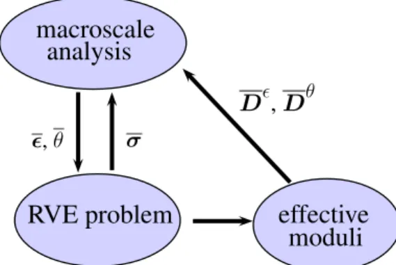
A complete homogenization scheme requires the solution of the macroscale and the microscale simultaneously. In figure 2 an iterative scheme for homogenization is shown. From the macroscale analysis the macroscopic strains and temperatures are obtained, which are used in the RVE pro-blem to compute the microscale variables and the correct macroscopic stresses. Moreover, the RVE problem provides information to compute the effective thermomechanical tan-gent moduli, which are used in the macroscale analysis. The proposed methodology is motivated from the return mapping
algorithm utilized to simulate the behavior of nonlinear materials (Simo and Hughes1998).
In the sequel, the expressions are simplified by presenting the variables without mentioning their dependence on posi-tions x and/or x.
3.1. Macroscale problem
At time step n everything is considered to be known. Con-sidering known temporal and spatial macroscopic temperature distribution throughout the composite, θ at time stepn+1is also known. The task of the macroscale problem is to evaluate the macroscopic strains at timen+ 1.
By introducing the space of the macroscopic test func-tions
=
{
η: η, gradη ∈ 2( )
¯ ,η =0on ∂¯EB}
, (15) where ∂¯EB⊂ ∂¯ denotes the part of the boundary surface where displacements are prescribed, the weak form of the macroscale problem is written as
∫
η σ∫
η η − = ∀ ∈ ∂ t V S grad : d · d 0, . (16) ¯ ¯NBIn the last expressiont =σ ·n is the external traction, acting on the surface∂¯NB⊂ ∂¯, that the overall body is subjected to. Equation (16) generally represents a nonlinear system of equations. In such cases a Newton–Raphson scheme is uti-lized and the consistent linearization yields
∫
∫
η σ η η δ + − = ∀ ∈ ϵ ∂ D u t V S grad : : grad d · d 0, , (17) m m m ¯ ( ) ( ) ( ) ¯NB ⎡⎣ ⎤⎦where m denotes the iteration step. In the preceding expres-sion the temperature does not appear, since it is known at time
+
n 1 and thus it has no increment during the Newton– Raphson scheme. If the macroscopic stress σ and the macro-tangent modulus Dϵ are known from the solution of the microscale problem, then equation (17) can be solved for δu and thus the macro-strains ϵ at time step n+1 can be obtained. A detailed algorithmic scheme for the macroscale problem is provided in tableA1of appendixA.
3.2. Microscale problem
Just as in the macroscale analysis, at time step n everything is considered to be known. The task of the microscale problem is to evaluate the microscopic behavior at time n+1 and necessary quantities for the macroscale analysis. Specifically, thefirst objective is to obtain the microscopic strains ϵ and the microscopic internal variables ζ (these can be, for example, the transformation strain tensor and the martensitic volume fraction in the case of the SMA material). The second objective is to obtain the macroscopic stresses and the mac-roscopic thermomechanical tangent moduli.
By introducing the space of the microscopic periodic test functions η η η η = ∈ ∂
{
: , grad ( ), periodic on }, (18) 2the weak form of the microscale problem is written as
∫
grad :η σdV=0, ∀ ∈η . (19) Equation (19) generally represents a nonlinear system of equations. In such cases a Newton–Raphson scheme is uti-lized and the consistent linearization yields
∫
η σ η δ δθ + + = ∀ ∈ ϵ θ D u D V grad : : grad d 0, , (20) * * * * * m m m m m ( ) ( ) ( ) ( ) ( ) ⎡ ⎣⎢ ⎤ ⎦⎥where m* denotes the iteration step. With the help of equation (11) the last relation is written
∫
η σ ϵ η δ δ δθ + + + = ∀ ∈ ϵ ϵ θ D z D D V grad : : grad : d 0, . (21) * * * * * * * m m m m m m m ( ) ( ) ( ) ( ) ( ) ( ) ( ) ⎡ ⎣⎢ ⎤ ⎦⎥At this point a methodology similar to the return mapping algorithm is used to solve the problem.
1. As a first step the strain and the macro-temperature are provided exclusively by the macroscale analysis, which means that the terms δ ¯ and δθ inϵ equation (21) are zero. Thus
∫
η σ η δ + = ∀ ∈ ϵ D z V grad : : grad d 0, . (22) * * * m m m ( ) ( ) ( ) ⎡ ⎣⎢ ⎤⎦⎥The material behavior of the constituents is described by appropriate constitutive law algorithms which, using the microscopic strain ϵ and the microscopic internal variables ζ of the previous iteration step, can provide updated values of the internal variables, as well as the micro-stressσand the micro-tangent moduliDϵ,Dθfor the next iteration step (see Simo and Hughes1998for plastic and viscoplastic materials and Lagoudas 2008
for SMA materials). Thus, equation (22) constitutes a
nonlinear system with regard to δz that can be solved iteratively. Once the convergence is achieved (i.e., the residual term
∫
grad :η σ(m*) dV is close to zero), themacroscopic stress is obtained from equation (10). The complete algorithm of thisfirst step (RVE problem) of the microscale analysis is given in table A2 of appendixA.
2. Once the first step is completed, the residual term is assumed exactly zero. The next step is to obtain the macroscopic tangent moduli that will allow us to proceed to an elastic prediction in the macroscale analysis. Thus, technically the terms δϵ and δθ are ‘released’ from being zero and equation (21) is written
∫
η ϵ η δ + δ + δθ = ∀ ∈ ϵ ϵ θ D z D D V grad : : grad : d 0, , (23) ⎡⎣ ⎤⎦where the micro-tangent moduli Dϵ, Dθ at each local micro-point are those obtained from the RVE problem after its convergence. Equation (23) has, up to a macroscopic constant, a solution of the form (Ene1983)
ϵ χ χ
δz=δ¯: ϵ +δθ θ. (24) In the preceding expression, χϵ is a third-order
corrector tensor which is computed from the solution of the system
∫
η χ η + = ∀ ∈ ϵ ϵ ϵ[
D D]
V grad : :˜ grad d 0, , (25)where :˜ denotes the non-standard double contraction operation between two fourth-order tensors L and M with[ :˜L M]ijkl =[ ]Lijpq[M]klpq. Additionally, χθ is a
vector corrector which is computed from the solution of the system
∫
η χ η + = ∀ ∈ ϵ θ θ D D V grad : : grad d 0, . (26) ⎡⎣ ⎤⎦Using equations (3), and (10), (13), and (24) and considering the symmetries of the tensors Dϵ and Dθ, the increment of the macroscopic stress is expressed as
∫
∫
∫
∫
∫
σ σ ϵ ϵ χ ϵ χ δ δ δ δθ δ δ δθ δ δθ = = + = + + = + + + ϵ θ ϵ ϵ θ ϵ ϵ ϵ ϵ θ θ[
]
D D D z D D D D D D V V V V V d : d : grad : d :˜ grad d : : grad d . (27) V V V V V 1 1 1 1 1 ⎡⎣ ⎤⎦ ⎡⎣ ⎤⎦ ⎡⎣ ⎤⎦Comparing the last expression and equation (7) leads to
∫
∫
χ χ = + = + ϵ ϵ ϵ ϵ θ ϵ θ θ[
]
D D D D D D V V :˜ grad d , : grad d . (28) V V 1 1 ⎡⎣ ⎤⎦microscale analysis (effective tangent moduli problem) is given in tableA3of appendixA.
It is worth mentioning that, while the macroscopic thermal tangent modulus tensor can be calculated with the present approach, it does not affect the macroscopic solution of the problem, since it does not enter in the iterative Newton– Raphson scheme for the macro-displacement. This tensor is useful in fully coupled thermomecanical analyses.
4. SMA constitutive law
The homogenization framework presented in the previous sections is independent of the choice of the constitutive laws for the material constituents. To illustrate the methodology through numerical examples, a choice of a SMA constitutive model is required that accounts for the phase transformation between austenite and martensite. Here the recent and pow-erful phase transformation model by Lagoudas et al (2012) is chosen for two reasons: a) it is robust, widely utilized and thermodynamically consistent and b) it has the ability to account for three-dimensional loading cases.
According to Lagoudas et al (2012), the SMA Gibb’s free energy functional depends on the stressσ and the tem-perature T, as well as on some internal variables. The chosen internal variables are the transformation strain ϵtr and the martensitic volume fractionξ. The total strain, ϵ, is decom-posed in three parts, the elastic, ϵel, the thermal ϵ ,th and the transformation strain, ϵtr,
ϵ=ϵel +ϵth+ϵtr. (29) The elastic strain is connected with the stress though the linear relation
ϵel = S( ): .ξ σ (30) ξ
S ( )is the compliance tensor of the SMA, which depends on ξ via a rule of mixtures relation
ξ = +ξΔ Δ = −
S( ) SA S, S SM SA, (31) where the superscripts M and A denote martensite and aus-tenite respectively. For isotropic SMAs the compliance tensor is a function of the Young moduli EA, EM and the Poisson ratiosνA,νM. The thermal strain is given by
ϵth=α θ
[
−θ0]
, (32) where θ0 is a reference temperature and α is the thermal expansion coefficient (same for austenite and martensite). With regard to the phase transformation, forward transfor-mation is the process in which the austenite is transformed into martensite (ξ >˙ 0) and reverse transformation is the process in which the martensite is transformed into austenite (ξ <˙ 0). The transformation strain is provided through anevolution law of the form
ϵ Λ Λ σ ϵ ξ σ ξ ξ ξ = = ′ > < − − H ˙ ˙, 3 2 , ˙ 0, , ˙ 0, (33) t r t r tr cur vM ⎧ ⎨ ⎪⎪ ⎩ ⎪ ⎪
where σ′ =σ− 13trace( )σ iis the deviatoric part of the stress tensor, σvM= 3σ′:σ′
2 is the von Mises effective stress tensor, ϵt r− is the transformation strain tensor at the end of the forward transformation, ξt r− is the martensitic volume frac-tion at the end of the forward transformafrac-tion (for complete transformation loops ξt r− = 1), and Hcur is a scalar material
parameter associated with the maximum transformation strain and is connected with σvM through the relation
σ σ σ σ = ⩽ + − − > σ σ − − H H H H H e , , 1 , . (34) cur k min vM crit
min sat min
vM crit vM crit ⎧ ⎨ ⎪ ⎪⎪ ⎩ ⎪ ⎪⎪ ⎡⎣ ⎤⎦⎡⎣⎢ ⎤ ⎦⎥ ⎡ ⎣ ⎤⎦
In the precedig expression, Hmin,Hsat, σcrit,and k are material parameters (for further details, see Lagoudas et al 2012).
Based on standard thermodynamics considerations, the model identifies the mechanical dissipation during forward and reverse transformation to be expressed as
πξ ⩾˙ 0. (35) In the last expressionπ is the thermodynamic force conjugate toξ. Assuming the same thermal expansion coefficients and heat capacities for austenite and martensite, this force is written as
σ Λ σ σ
π= : + 1 ΔS +ρΔs −ρΔu −f
2 : : 0 0 , (36)
where ρ is the density, Δs0 is the change of the effective specific entropy between the austenite and martensite, Δu0is the change of the effective specific internal energy between the austenite and martensite, and f is a smooth transformation hardening function, ξ ξ ξ ξ ξ ξ = + − − + > + − − − <
[
]
[
]
f a a a a 1 2 1 [1 ] , ˙ 0, 1 2 1 [1 ] , ˙ 0. (37) n n n n 1 3 2 3 1 2 3 4 ⎧ ⎨ ⎪⎪ ⎩ ⎪⎪In the preceding expression, n1-n4are exponents related to the
smoothness of the function and a1-a3are material parameters
connected to the two phase diagram slopes, CAand CM, and the four transformation temperatures: martensitic start Ms,
martensitic finish Mf, austenitic start As, and austeniticfinish
Af(for further details, see Lagoudas et al2012). Both forward
and reverse transformation processes are limited by the value ofξ, which should be between 0 and 1. For the forward and reverse transformation processes appropriate plasticity-type functions Φforward and Φreverse are identified, accompanied by
Kuhn–Tucker conditions, ξ Φ π ξΦ ξ Φ π ξΦ ⩾ = − ⩽ = ⩽ = − − ⩽ = Y Y ˙ 0, 0, ˙ 0, ˙ 0, 0, ˙ 0, (38) forward forward reverse reverse
where Y is a material parameter similar to the yield stress in plasticity.
Providing (a) the total strain ϵ and temperatureθ at time stepn+1, (b) the transformation strain ϵtr and (c) the mar-tensitic volume fraction ξ at time step n, the system of equations (29), (30), (33), and (38) can be solved iteratively through a numerical scheme (for instance the convex cutting plane return mapping algorithm) to identify the stressσ, the transformation strain ϵtrand the martensitic volume fractionξ at time step n+1. Once these quantities are known, the continuum tangent modulus Dis computed and used for the next elastic prediction in the RVE problem. Additional details on the numerical implementation of the model can be found in Lagoudas (2008).
One disadvantage of the specific SMA model is that it cannot handle minor loops in the transformation regime. Thus, in all the proceeding analyses the loading and unloading conditions guarantee fully forward and fully reverse transformations, respectively.
5. Composite laminate with SMA constituents: isothermal case
This section studies the macroscopic behavior of a composite laminate, whose RVE includes an SMA material with volume fraction c and another metallic material with volume fraction
− c
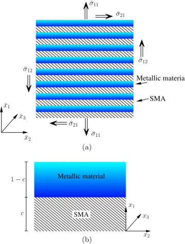
1 (figure3(b)). In the following studied cases, the com-posite is subjected to a combination of a normal macroscopic stressσ11in thex¯1direction (normal to the layers) and a shear macroscopic stressσ12, asfigure3(a) depicts.
The RVE and the effective tangent modulus problems of a composite laminate are reduced to systems of one-dimen-sional differential equations and they have an analytical or semi-analytical solution (see for example Chatzigeorgiou et al2014in the case of composites with energetic interfaces). For manuscript completeness, appendixB presents the solu-tions of these problems for a laminate composite with N layers exhibiting nonlinear behavior.
Due to the applied macroscopic stress boundary condi-tions, the complete homogenization problem needs to be solved iteratively and simultaneously in both micro- and macroscale levels, as the procedure described in section 3
indicates: The macroscopic boundary condition must be imposed incrementally. In the first step, the application of macroscopic stress leads to a triaxial normal and shear strain response. In the second step, this macroscopic strain tensor is implemented into the RVE problem to obtain the corrected macroscopic stress and the effective tangent modulus. The process continues iteratively until the corrected stress is approximately equal to the applied stress. Once this is achieved, the procedure continues with the next time increment.
In the numerical examples that follow, a SMA material is chosen, whose properties are summarized in table 1. For simplicity in obtaining the stress levels at the onset andfinish of transformations, the smoothness of the hardening function has been removed by setting all the transformation exponents equal to 1. Figure 4 shows the pure SMA pseudoelastic response at 300 K under uniaxial macroscopic loading and its phase diagram. All demonstrated results in the examples of this section are obtained for constant temperature, equal to 300 K, and for zero thermal strains. The numerical examples have been performed using a developed c++ code, based on the theory and numerical scheme presented previously. Figure 3.Schematic representation of (a) a multilayered material with SMA constituents under tension—shear loading and (b) the RVE of the composite.
Table 1.Material properties of SMA (Lagoudas2008). Property Austenite Martensite
Young modulus (GPa) 55 46
Poisson ratio 0.33 0.33 Ms(K) 245 Mf(K) 230 As(K) 270 Af(K) 280 n1,n2 1 n3,n4 1
Phase diagram slope (MPa/K) 7.4 7.4 =
Hmin Hsat
5.1. Laminate with SMA and elastic material
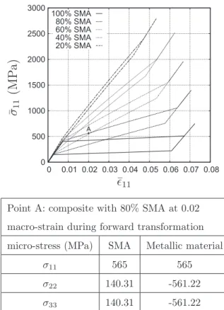
In thefirst series of examples the metallic material is assumed to be elastic with a Young modulus of 69 GPa and a Poisson ratio of 0.3. Figure 5 demonstrates the macroscopic stress-strain response of the multilayered composite when subjected to pure tension, forfive different SMA volume fractions, 100 (pure SMA), 80, 60, 40 and 20%. From these curves it is clearly observed that the decrease of the SMA volume frac-tion reduces the hysteresis of the composite response, and decreases the maximum transformation strain. Due to the elastic response of the metallic material, the stress levels required to complete the transformation of a composite with significant metallic material volume fraction are extremely high and thus other type of phenomena should also appear (development of plastic strains, damage, etc).
Another relevant observation is that even though the composite is under uniaxial stress state, the material con-stituents, at the RVE scale, are locally subjected to a non-proportional triaxial stress state (see table infigure5, as well asfigure8). This could significantly affect the SMA response and would trigger other types of mechanisms, like martensitic variant reorientation, that the present SMA model cannot capture.
Infigure6the macroscopic stress-strain response of the composite laminate when subjected to simple shear is pre-sented. It is observed that the decrease of SMA content in the composite decreases the hysteretic response, but does not alter the stress levels that forward and reverse transformations start andfinish.
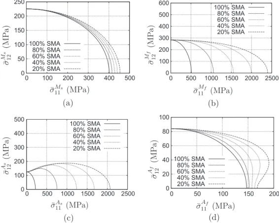
Figure 7 illustrates the transformation characteristics under combined shear-tension macro-loading conditions. Specifically, the decrease of SMA volume fraction in the composite does not seem to influence significantly the onset of forward transformation (figure7(a)), but it causes drastic changes at the end of forward and the onset of reverse transformation (figures 7(b) and 7(c), respectively). Further-more, it should be noticed that, for SMA volume fractions below 60%, the end of reverse transformation presents a non-convex response (figure7(d)). This peculiar behavior arises as the result of the extreme non-proportionality in the stress Figure 4.(a) SMA pseudoelastic response at 300 K under uniaxial
tension loading-unloading conditions, (b) SMA phase diagram.
Figure 5.Composite response under pure tension macro-loading at various SMA volume fractions and RVE response at specific macro-strain conditions.
Figure 6.Composite response under simple shear macro-loading at various SMA volume fractions.
response of the SMA. Figure 8 shows the micro-stresses in two directions (normal and parallel to the layers) inside the SMA constituent for a composite with 80% metallic material volume fraction. It is observed that, when the SMA is not transforming, the σ11 is the dominant normal stress. During the transformation on the other hand, the incompressibility of the transformation strains and the loading requirement that the macroscopic stress σ22 must be zero cause a significant increase of the micro-stress σ22 in the SMA leading to be almost equal (at the end of forward transformation), and even exceeding the normal stress σ11 (at the beginning of reverse transformation). This alteration of the micro-stresses analogy causes a complicated loading path and, asfigure8depicts, the
finish of reverse transformation for two different macroscopic loading conditions (100% tension and 80% tension-20% shear) appears almost at the same stress level. So it becomes clear that even for simple macroscopic loading conditions, the microscopic response at each phase can be very complicated and strongly non-proportional. Thus, while the SMA con-stitutive law ensures a convex SMA response at all times (as figure 7 depicts for 0% metallic material), there is no guar-antee that the average (overall) response of the composite will behave in the same way. The SMA constituent drives the start and finish of transformation of the composite, but the stress state of the two cannot be linked intuitively, and it is possible to observe a peculiar average response without violating the convexity of the materials in the microscale. In the occasion of low SMA content in the composite, the macroscopic response is driven mainly by the elastic material, while the transformation characteristics still depends on the SMA material, causing more disturbance in the overall transfor-mation surfaces, compared to composites with high SMA content (figure7).
Curves like the ones presented in figure7 can be very useful for designing a phenomenological macroscopic model for the composite response. In such a model the material constants could be identified through an appropriate para-meter identification method (Meraghni et al2014). Of course, special attention needs to be taken when non-convex com-posite transformation surfaces appear.
Figure 7.Shear versus normal macro-stress at (a) start of forward transformation, (a)finish of forward transformation, (c) start of reverse transformation, and (d)finish of reverse transformation.
Figure 8.Multilayered composite with 20% SMA volume fraction: normal micro-stresses inside the SMA for i) uniaxial macroscopic tension and ii) 80% σ11-20% σ12.
5.2. Laminate with SMA and elastoplastic material
In the second series of examples the metallic material presents elastoplastic Von–Mises response with a linear isotropic hardening. Its elastic properties remain the same, while for the plastic behavior a yield stress 275 MPa and a linear hardening 12 GPa are assumed. The uniaxial macroscopic stress strain curve of the pure metallic material is shown infigure9.
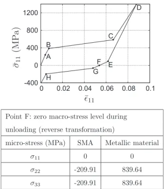
The following analysis considers zero macroscopic shear loading. The elastoplastic constitutive law of the matallic material is described through a convex cutting plane return mapping algorithm (Simo and Hughes1998). Infigure10the overall response of the composite with 80% SMA and 20% metallic material is presented. At the initial step the composite is loaded in tension and both the SMA and the metallic material are behaving elastically. At point A of the curve the metallic material starts developing plastic strains and there is a slight change in the slope of the curve. At point B the SMA
starts transforming and this process continues until point C, where all austenite has been transformed into martensite. Then until point D the SMA behaves elastically and the metallic material behaves plastically. During unloading the metallic material behaves elastically, that is why two different slopes at point D are observed. At point E the metallic material continues to be in an elastic state but the SMA enters in the reverse transformation. At point G the metallic material enters again in the plastic region, while the SMA still trans-forms. The reverse transformationfinishes at point H and the composite returns to zero macroscopic ϵ11 strain when the macroscopic σ11 stress is approximately 400 MPa in compression.
It must be noticed that at zero macro-stress level the SMA material is in a biaxial compression state (see table in figure10). Thus, it is important to know if the SMA material response presents tension-compression asymmetry in order to obtain the correct overall response, even if the composite is loaded only under macroscopic tension conditions.
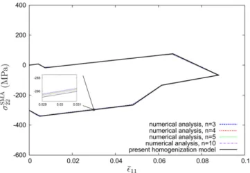
To verify the results of the homogenization method, a numerical analysis is performed for a composite laminate with n number of RVEs using the commercial finite element software ABAQUS. This computational procedure solves the whole composite (not only the RVE) using the macroscopic boundary conditions. Thus, it can be considered as the reference solution for the composite response, independently of any homogenization scheme.
According to the homogenization theory, as the number n increases, the average response of the composite should attain asymptotically the response predicted by the homogenization procedure. In the current study n takes the values 3, 4, 5, and 10. To facilitate the process, all boundary value problems for various n were generated through an appropriate python script. For n = 5,figure11shows thefinite element mesh that consists of 20 000 quadratic elements C3D20R in total. The boundary conditions of the composite are considered the macroscopic ones, i.e., uniform traction along the axis normal to the layers. The analysis in ABAQUS confirms the accuracy of the homogenization scheme. The finite element results appear to be insensitive to the number of RVEs and both the macroscopic response (figure12) and the microscopic stress
σ22 in the SMA constituent (figure13) are predicted correctly from the homogenization method. In thefinite element ana-lysis, σ22SMArefers to the average σ22 stress component of an Figure 9.Metallic material elastoplastic response under uniaxial
loading-unloading conditions.
Figure 10.Mutilayered composite with 80% SMA volume fraction: Composite response under pure tension macro-loading and RVE response at zero macro-stress during unloading.
Figure 11.Laminate composite with 80% SMA volume fraction and n = 5 (5 SMA layers and 5 metallic material layers). Finite element mesh in ABAQUS. The normal displacements at the bottom, left, and behind surfaces are constrained (roller support), while the upper surface is subjected to traction.
arbitrary SMA layer2. Thus, the large computational cost of the finite element procedure (which is even higher for strongly nonlinear SMA laws) can be avoided by utilizing the described homogenization methodology, which allows us to obtain very accurately the actual composite response.
In the previous analysis the plastic yielding of the metallic material started earlier than the SMA transformation. In the next example the yield stress of the metallic material is tripled (825 MPa), while keeping the same composite synth-esis and metallic material hardening slope. The resulting composite response is illustrated infigure14. As in the pre-vious example, at the initial step of the macro-tension loading both the SMA and the metallic material behave elastically. At point A’ of the macroscopic curve the SMA starts trans-forming and there is an important change in the slope of the curve. At point B’ the metallic material starts developing
plastic strains. At point C’ all austenite has been transformed into martensite. Then, until the point D’ the SMA behaves elastically and the metallic material behaves plastically. At the first steps of unloading the metallic material behaves elasti-cally, which again causes the appearance of two different slopes at point D’. At point E’ the metallic material continues to be in the elastic state but the SMA starts the reverse transformation. At point G’ the metallic material enters again in the plastic region, while the SMA is still under transfor-mation, until itfinishes at point H’.
6. Composite laminate with SMA constituents: isobaric case
In the following example, composite laminates are studied under a quasi-static thermomechanical cycle. Since the velo-cities are considered very low, latent heat and heat transfer effects will be ignored. The examined composites consist of nickel-rich NiTi, whose properties are summarized in table2, and epoxy with properties given in table 3. The numerical example starts at temperature 400 K and the followed loading path has 4 steps:
Figure 12.Laminate composite with 80% SMA volume fraction: Comparison between numerical analysis with ABAQUS and homogenization scheme. Macroscopic stress σ11versus macroscopic
strain ϵ11.
Figure 13.Mutilayered composite with 80% SMA volume fraction: Comparison between numerical analysis with ABAQUS and homogenization scheme. SMA stress σ22versus macroscopic strain
ϵ11.
Figure 14.Mutilayered composite with 80% SMA volume fraction and increased metallic material yield stress: Composite response under pure tension macro-loading.
Table 2.Material properties of nickel-rich NiTi (Lagoudas et al2012).
EA(GPa) EM(GPa) νA νM
90 63 0.3 0.3
Hmin
Hsat k (1/MPa) σcrit(MPa)
0 0.016 0.0075 12 Ms(K) Mf(K) As(K) Af(K) 308 242 288 342 n1 n2 n3 n4 0.6 0.2 0.2 0.3 CA(MPa/K) CM(MPa/K) α (1/K) θ0(K) 16 10 1.0E-5 400
Table 3.Material properties of epoxy. E (GPa) ν α (1/K) θ0(K)
3.85 0.4 4.4E-5 400
2 For consistency reasons, it always used the second SMA layer starting
1. loading up to a stress level of 200 MPa in the direction 1,
2. cooling until the temperature reaches 200 K, 3. heating until the temperature reaches 400 K, and 4. unloading to zero stress level.
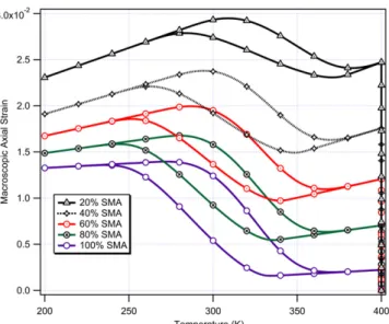
The strain-temperature diagram of the analysis is illustrated in figure15for pure SMA and for composites with 20, 40, 60 and 80% epoxy. The results indicate that the increase of the epoxy volume fraction increases the strain levels and decreases the maximum transformation strain of the compo-site. Also the transformation temperatures increase signi fi-cantly at low SMA volume fractions, which indicates that the stress level inside the alloy has increased substantially.
7. Summary and conclusions
The following points summarize this paperʼs goals:
• This work introduced a computational homogenization approach, based on the periodic homogenization theory, for composites with SMA constituents. The proposed methodology identifies the macro- and micro-responses of the composites under quasi-static thermomechanical conditions, independently of the micro-geometry and the macroscopic boundary conditions.
• The proposed homogenization framework was tested in the case of composite laminates, where semi-analytical solutions are available, and both the macro and micro-responses showed excellent agreement with those obtained by finite element analysis performed in structures with multiple RVEs. This agreement is practically insensitive to the number of RVEs of the structure, thus the current model can be used for laminate materials with small number of layers. The proposed
method allows us to avoid the computational cost of the FE analysis, which is enlarged by the complexity of the SMA constitutive law, without reducing the accuracy in the prediction of the composite response.
The numerical examples on the current study illustrated that even for simple uniaxial macroscopic boundary condi-tions the SMA components can be in triaxial stress state. Thus, to capture accurately the behavior of the composite, it is very important to account for possible anisotropic behavior of the SMA constituents, as well as other type of mechanisms like the martensitic variant reorientation. Computations on composite laminates with SMA and metallic material (elastic) components revealed that the transformation criteria of the composite can be significantly different from that of a typical SMA. An interesting observation is that at the finish of reverse transformation a non-convex macroscopic response appeared at high metallic material content. The results for multilayered materials with SMA and metallic material (elastoplastic) components showed complex macroscopic response, with significant interactions between the transfor-mation and the plasticity. The sequence of the appearance of the nonlinear micro-mechanisms depends on the yield stress of the metallic material and the activation stresses of the SMA (start and finish of forward and reverse transformation). Finally, thermomechanical loading paths on composite lami-nates indicate that the presence of elastic components can change drastically the transformation temperatures at specific stress levels, compared to the pure SMA behavior.
Future extensions of this work could include analyses of SMA composites with more complicated microstructures (particle, fiber, woven composites), as well as the incor-poration of other type of nonlinear mechanisms (for instance, damage). Additionally, the interplay between the mechanical and thermal effects will be examined through a fully coupled thermomechanical analysis.
Acknowledgments
The authors would like to thank Ali Javili (Chair of Applied Mechanics, Friedrich-Alexander University of Erlangen-Nuremberg) for helpful discussion.
Appendix A. Numerical algorithms for periodic homogenization
The numerical algorithms presented in this appendix have similar structure with those presented in Tsalis et al2013for the case of elastoplastic media with generalized periodicity. The symbol ζ denotes the internal variables of the material constituents that appear in an RVE (in an elastoplastic material these can be the plastic strain tensor and the equivalent plastic strain, in a shape memory alloy these can be the transformation strain tensor and the martensitic volume fraction). In tableA2the constitutive law algorithm can be a classical return mapping algorithm that computes the stress, Figure 15.Macroscopic strain ϵ11-temperature curves for pure SMA
and composites with various SMA volume fraction during a complete thermomechanical loading cycle.
the tangent thermomechanical moduli, and the change of the internal variables for given strain and initial values of ζ (see Simo and Hughes 1998 for elastoplastic or viscoplastic materials and Lagoudas2008for SMAs) .
Appendix B. Solution of the RVE and the effective mechanical tangent modulus problems for a composite laminate
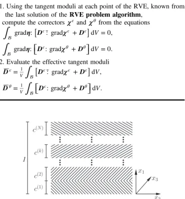
Similar solution strategies for composite laminates with linear material constituents, using the periodic homogenization method, have been presented in the literature by several authors (see for instance Kalamkarov and Kolpakov1997in the case of laminated plates). For the completeness of the manuscript, this appendix presents the semi-analytical solu-tion for the RVE and the tangent moduli problems. The effective thermal tangent modulus is omitted, because it was not utilized in the performed analyses, but its computation follows similar steps with the mechanical one.
A composite laminate, whose RVE consists of N con-stituents, is demonstrated infigureB1. Each constituent has volume fractionc( )k and mechanical tangent modulus Dϵ( )k
( =k 1, 2,…,N). Obviously ∑rN= cr =1 1
( ) . For simplicity, in all the subsequent expressions the iteration step is omitted and only the material that the quantity refers to is defined.
RVE problem
In the RVE of the multilayered material and under periodicity conditions the periodic part of the displacement, δz, is
uniform along the x2and x3axes and presents non-uniformity
only on the x1 axis. Thus, equation (22) can be substituted
with its local form for each material k ( =k 1, 2,…,N), which is the one-dimensional differential equation system
σ δ + = ϵ D z x x 0 d d · d d , (B.1) nn k k n k 1 ( ) ( ) 1 ( ) ⎛ ⎝ ⎜ ⎞ ⎠ ⎟ with σ σ σ σ = = ϵ ϵ ϵ ϵ ϵ ϵ ϵ ϵ ϵ ϵ D D D D D D D D D D and . (B.2) nn k k k k k k k k k k n k k k k ( ) 1111 ( ) 1121 ( ) 1131 ( ) 2111( ) 2121( ) 2131( ) 3111( ) 3121( ) 3131( ) ( ) 11 ( ) 21( ) 31( ) ⎡ ⎣ ⎢ ⎢ ⎢ ⎤ ⎦ ⎥ ⎥ ⎥ ⎡ ⎣ ⎢ ⎢ ⎢ ⎤ ⎦ ⎥ ⎥ ⎥
Due to the continuity of tractions, the system (B.1) after integration is written σ σ + = = − ϵ δ δ ϵ − D m D m · , or · , (B.3) z z nnk x nk x nn k nk ( ) d d ( ) d d ( ) 1 ( ) k k ( ) 1 ( ) 1 ⎡⎣ ⎤⎦ ⎡⎣ ⎤⎦
where m is a constant vector independent of the material. Integrating once more the solution of the system is obtained in the form σ δzk = Dϵ − · m− x +e , (B.4) nnk nk k ( ) ( ) 1 ( ) 1 ( ) ⎡⎣ ⎤⎦ ⎡⎣ ⎤⎦
where e( )k are constant vectors that depend on the material.
Thefinal expression indicates thatδz( )k are linear functions of
x1. Considering periodicity of the vector δz( )k it can be
assumed, without loss of generality, that
δz(1)(0)= δz( )N (1) =0, which leads to σ = = − ϵ − − e 0, eN D · m . (B.5) nn N n N (1) ( ) ⎡⎣ ( )⎤⎦ ⎡⎣1 ( )⎤⎦
The continuity ofδz( )k at all the interfaces is expressed by the
relation
δz( )k
( )
c( )k =δz(k+1)( )
c( )k , k=1, 2,…,N−1. (B.6) Using equations (B.4), (B.6) is expressed for each interface asσ σ σ σ σ σ − = − + − + + = − + + − + + + = − + + + ϵ ϵ ϵ ϵ ϵ ϵ − − − − − − D m D m e D m e D m e D m e D m e c c c c c c c c c c c c · · , · · , · · , nn n nn n nn n nn n nn n nn n (1) 1 (1) (1) (2) 1 (2) (1) (2) (2) 1 (2) (1) (2) (2) (3) 1 (3) (1) (2) (3) (3) 1 (3) (1) (2) (3) (3) (4) 1 (4) (1) (2) (3) (4) ⎡⎣ ⎤⎦ ⎡⎣ ⎤⎦ ⎡⎣ ⎤⎦ ⎡⎣ ⎤⎦ ⎡⎣ ⎤⎦ ⎡⎣ ⎤⎦⎡⎣ ⎤⎦ ⎡⎣ ⎤⎦ ⎡⎣ ⎤⎦⎡⎣ ⎤⎦ ⎡⎣ ⎤⎦ ⎡⎣ ⎤⎦⎡⎣ ⎤⎦ ⎡⎣ ⎤⎦ ⎡⎣ ⎤⎦⎡⎣ ⎤⎦
Table A1.Macroscale analysis algorithm. 1. At time step n everything is known. At time stepn+1 and
iteration step m = 0 set Δu + =
0
n
( 1)(0) , ϵ¯(n+1)(0)= ϵ¯( )n,
σ¯(n+1)(0)=σ¯( )n, Δθ(n+1)=θ(n+1)−θ( )n
.
2. In an RVE at each macroscopic point call the effective tangent moduli algorithmand obtainDϵ(n+1)( )m, Dθ(n+1)( )m.
3. Compute the virtual increment of u from the macro-equilibrium equation
∫
∫
η σ η δ + − = ϵ + + + ∂ + D u t V S grad ¯: : grad ¯ d ¯ · d 0. n m n m n m n ¯ ( 1)( ) ( 1)( ) ( 1)( ) ¯ ( 1) NB ⎡⎣ ⎤⎦4. Update the macro-quantities Δu(n+1)(m+1)=Δu(n+1)( )m +δu(n+1)( )m, ϵ δ¯(n+1)( )m =grad δun+ m sym ( 1)( ), ϵ¯(n+1)(m+1)=ϵ¯(n+1)( )m +δϵ¯(n+1)( )m.
5. At each macroscopic point, call the RVE problem algorithm and compute σ¯(n+1)(m+1). 6. If
⏟
δ Δ ∥ u + ∥ ∥ u + + ∥ ⩽ max tol V n m n m ( 1)( ) ( 1)( 1)then compute the macro-displacementu(n+1)=u( )n +Δu(n+1),
update the values of ϵ(n+1), ζ(n+1)of the RVE problem,
setn=n+1 and return to step 1, else setm=m+1 and return to step 2.
∑
∑
∑
∑
∑
∑
σ σ σ σ σ σ σ ⋮ − + = − + − + = − + ⋮ − + = − − − ϵ ϵ ϵ ϵ ϵ ϵ ϵ − = + − + = + + − + = + + + − + = + + − − − = − − − = − − D m e D m e D m e D m e D m e D m D m c c c c c c · · , · · , · · · . nnk nk r k r k nnk nk r k r k nnk nk r k r k nnk nk r k r k nnN nN r N r N nnN nN r N r nnN nN ( ) 1 ( ) 1 ( ) ( ) ( 1) 1 ( 1) 1 ( ) ( 1) ( 1) 1 ( 1) 1 1 ( ) ( 1) ( 2) 1 ( 2) 1 1 ( ) ( 2) ( 1) 1 ( 1) 1 1 ( ) ( 1) ( ) 1 ( ) 1 1 ( ) ( ) 1 ( ) ⎡⎣ ⎤⎦ ⎡⎣ ⎤⎦ ⎡⎣ ⎤⎦ ⎡⎣ ⎤⎦ ⎡⎣ ⎤⎦ ⎡⎣ ⎤⎦ ⎡⎣ ⎤⎦ ⎡⎣ ⎤⎦ ⎡⎣ ⎤⎦ ⎡⎣ ⎤⎦ ⎡⎣ ⎤⎦ ⎡⎣ ⎤⎦ ⎡⎣ ⎤⎦ ⎡⎣ ⎤⎦Adding all the previous expressions leads to
∑
ϵ −σ = = − D · m c 0, r N nn r n r r 1 ( ) 1 ( ) ( ) ⎡⎣ ⎤⎦ ⎡⎣ ⎤⎦ orTable A2.RVE problem algorithm.
1. At macroscale stepm+1 and time stepn+1, ϵ¯(n+1)(m+1)
and θ(n+1)are known.
At microscale iteration stepm*=0 set Δz(n+1)(m+1)(0)=0, ϵ(n+1)(m+1)(0)=ϵ( )n +ϵ¯(n+1)(m+1)−ϵ¯( )n, ζ(n+1)(m+1)(0)=ζ( )n.
Evaluate the micro-stresses σ(n+1)(m+1)(0)and the micro-tangent
thermomechanical moduli Dϵ(n+1)(m+1)(0), Dθ(n+1)(m+1)(0)
using the constitutive law algorithm.
2. Compute the virtual increment of z from the micro-equilibrium equation
∫
∫
η η σ δ + = ϵ + + + + + + D z V V grad : : grad d grad : d 0. * * * n m m n m m n m m ( 1)( 1)( ) ( 1)( 1)( ) ( 1)( 1)( )3. Update the micro-quantities
Δz(n+1)(m+1)(m*+1)=Δz(n+1)(m+1)(m*)+δz(n+1)(m+1)(m*),
ϵ
δ (n+1)(m+1)(m*)=grad δzn+ m+ m*
sym ( 1)( 1)( ),
ϵ(n+1)(m+1)(m*+1)=ϵ(n+1)(m+1)(m*)+δϵ(n+1)(m+1)(m*).
4. At each microscopic point in the RVE, obtain the micro-stresses σ(n+1)(m+1)(m*+1)and the micro-tangent moduli
ϵ + +
D(n 1)(m 1)(0),Dθ(n+1)(m+1)(0)
using the constitutive law algorithm.
5. If
⏟
δ Δ ∥ z + + ∥ ∥ z + + + ∥ ⩽ max * * tol V n m m n m m ( 1)( 1)( ) ( 1)( 1)( 1)then continue with step 6,
else setm*=m*+1 and return to step 2.
6. Compute the periodic part of the micro-displacement, Δ
= +
+ + + +
z(n 1)(m 1) z( )n z(n 1)(m 1).
7. Compute the macro-stress, σ¯n+ m+ =
∫
σ + + dVV
n m
( 1)( 1) 1 ( 1)( 1) .
Table A3.Effective tangent moduli algorithm.
1. Using the tangent moduli at each point of the RVE, known from the last solution of the RVE problem algorithm,
compute the correctors χϵand χθ
from the equations
∫
∫
η χ η χ + = + = ϵ ϵ ϵ ϵ θ θ[
D D]
D D V V grad : :˜ grad d 0, grad :⎡⎣ : grad ⎤⎦d 0. 2. Evaluate the effective tangent moduli
∫
∫
χ χ = + = + ϵ ϵ ϵ ϵ θ ϵ θ θ[
]
D D D D D D V V :˜ grad d , : grad d . V V 1 1 ⎡⎣ ⎤⎦Figure B1.Schematic representation of the RVE of a composite laminate with N layers.