Science Arts & Métiers (SAM)
is an open access repository that collects the work of Arts et Métiers Institute of
Technology researchers and makes it freely available over the web where possible.
This is an author-deposited version published in:
https://sam.ensam.eu
Handle ID: .
http://hdl.handle.net/10985/11334
To cite this version :
Samuel BIGOT, Jean-Philippe PERNOT, Anthony SURLERAUX, Ahmed ELKASEER -
Micro-EDM numerical simulation and experimental validation - In: 10th International Conference on
Multi-Material Micro Manufacture (4M’13), Espagne, 2013 - Proceedings of the 10th International
Conference on Multi-Material Micro Manufacture - 2013
Any correspondence concerning this service should be sent to the repository
Administrator :
[email protected]
Micro-EDM numerical simulation and experimental validation
Samuel Bigot
1, Jean-Philippe Pernot
2, Anthony Surleraux
1, Ahmed Elkaseer
1
1 Manufacturing Engineering Centre, Cardiff University, Cardiff, UK, e-mail: [email protected] 2 Arts et Métiers ParisTech, LSIS − UMR CNRS 7296, Aix-en-Provence, France
Abstract
This paper introduces a new method for simulating the micro-EDM process in order to predict tool wear. The tool and workpiece are defined by NURBS surfaces whose shapes result from an iterative crater-by-crater deformation technique driven by physical parameters. The simulation method is validated through a comparison with experimental data. Different simulations are presented with an increase in computation accuracy in order to study its influence on the results and their deviation from expected values.
Keywords: Micro electrical discharge machining, crater, wear, simulation, NURBS surface deformation.
1.Introduction
Electrical Discharge Machining (EDM) is a manufacturing process that consists in removing parts of a material with electrical discharges and is characterized by its ability to machine any conductive material regardless of its hardness.
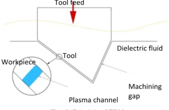
Although various forms of EDM exist all of them share the same concept: two electrodes (the tool and the workpiece) are separated by a dielectric fluid. Both electrodes are submitted to an electrical current and as the gap between the electrodes diminishes, the intensity between them increases until it reaches what is called the dielectric breakdown voltage. At this point, the dielectric cannot act as an insulator anymore and allows current to flow from one electrode to another leading to the apparition of a plasma channel. The plasma’s temperature ranges from 8,000 to 12,000°C and in some cases can reach up to 20,000°C [1]. This leads to evaporation and melting of both the tool and the workpiece. When the current is stopped, the dielectric fluid rushes back where the plasma stood and evacuates resulting debris.
Micro-EDM (µEDM) shares the same underlying concepts of EDM. It simply tackles with dimensions in the order of the micron.
Tool Tool feed Workpiece Machining gap Plasma channel Dielectric fluid Fig. 1. Principle of EDM
However, while the process setup is modified in order to reduce its effect, tool wear often becomes the main factor of imprecision. When using conventional machining strategies, the electrodes’ shapes quickly deviates from the original ones. Thus, as of now µEDM milling is the preferred machining strategy for the fact that proven methods [2] exist to mitigate the influence of tool wear on the final result, while for similar applications die-sinking µEDM may require a dozen or more tools before obtaining the desired geometrical tolerances.
Being able to predict the tool wear more accurately would enable us to design more efficient machining strategies, in particular for die sinking EDM where using extra volumes on specific parts of a tool electrode could compensate partially for the wear and drastically reduce the number of electrodes required. To achieve this, a better theoretical understanding of the wear phenomena is required. Thus, in a previous work [3] it was proposed to develop a new modelling framework to facilitate the development and validation of theoretical models of the wear and a new simulation method was introduced that uses two Non-Uniform Rational B-Splines (NURBS) surfaces to simulate the evolution of the resulting tool and workpiece shapes using a crater-by-crater iterative deformation technique. In this paper, a new version of this simulation method (section 2) is described and its performance is compared with the results obtained from several EDM experiments (section 3).
2.Micro-EDM simulation
2.1. Overview of the new simulation process
In the proposed approach, both the geometry of the tool and the geometry of the workpiece are defined by means of NURBS patches (see [5] for a complete description of the underlying mathematical
models). To allow the insertion of thousands of craters, the surfaces of the tool 𝑺" and workpiece 𝑺# are heavily refined using the Boehm’s knot insertion algorithm [5]. As a result the surfaces’ control points will be a lot closer to it hence local control is significantly increased. At each step of the insertion process the location of each crater (one on each electrode) is determined while identifying the shortest distance between the tool and the workpiece since it is considered that the electrical spark will happen on the less resistive path, i.e. the shortest one.
Minimum distance computations are done using an optimization method known as particle swarm optimization (PSO) which is a simple numerical optimizer that does not require the use of the gradient of the objective function [4]. A crater is then inserted in each of those locations by moving the surrounding control points. If the computed minimum distance exceeds the value of the minimum distance required for a spark to appear (known in EDM as the gap distance M%) then the tool is moved down along the 𝒛 axis with an increment of ∆(. Otherwise, if the computed minimum distance is smaller than M% then the PSO algorithm returns four values (𝑢", 𝑣") and (𝑢#, 𝑣#) corresponding to the parametric coordinates of the craters’ centres respectively on the tool (subscript 𝑡) and workpiece (subscript 𝑤). The algorithm then moves the control points located in the surrounding of the craters’ centres so that two craters of volumes 𝑉" and 𝑉# are inserted into the tool and workpiece. The deformation technique is similar to surface warping [5] considered as a geometric deformation technique [6]. The process ends when the desired depth D2 is met. The overall algorithm can be described in pseudo-code form as follows:
Initialization: M%, D2, ∆(, 𝑉", 𝑉# While (actual depth < D2)
(𝑑, 𝑢", 𝑣", 𝑢#, 𝑣#) = min_distance(𝑺", 𝑺#) If (𝑑 < M%) then
Entering the loop for inserting the 𝑘"6 craters on both surfaces 𝑺7 with 𝑖 ∈ {𝑡, 𝑤}:
Compute warping vectors 𝝎7[>]
Compute spheres centres’ positions 𝑪7[>] Identify the 𝑁7[>] control points of 𝑺7 to be moved in the 𝝎7[>] direction
For each control point 𝑷7,C[>], 𝑗 ∈ {1, … , 𝑁7>} and 𝑖 ∈ {𝑡, 𝑤}:
Compute the deviation 𝑟7,C[>] from 𝝎7[>] Compute warping value 𝑓7,C[>](𝑟7,C[>]) Move control point along 𝝎7[>] so that its
new position 𝑷7,C[>] is defined by: 𝑷7,C[>]= 𝑷7,C[>]+ 𝑓7,C[>] 𝑟7,C> . 𝝎7[>] End for Else move_tool_down(𝑺", ∆() End if End while
The different steps of the crater insertion process are further detailed in the next subsection.
2.2. Volume computation and crater insertion
For a given depth of the tool, if the minimum distance is smaller than the gap distance, the craters insertion process starts. One crater will be inserted on each surface 𝑺7 (𝑖 ∈ {𝑡, 𝑤}) and centred on 𝑺7(𝑢7, 𝑣7). For sake of clarity, the superscript [𝑘] has not been put on the parametric coordinates 𝑢7 and 𝑣7 even if these values refer to the 𝑘"6 craters (one on each surface).
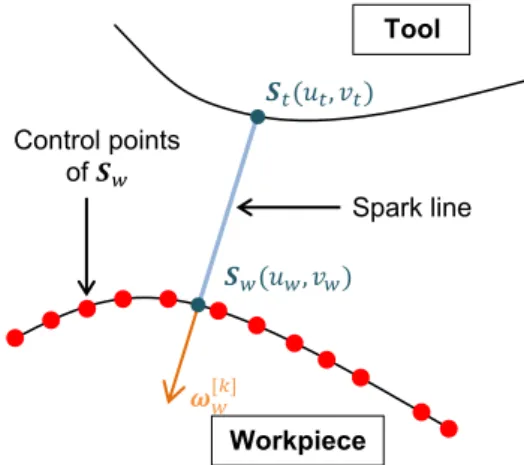
First, to identify the displacement directions, the two warping unit vectors are computed as follows:
𝝎7> = sg 𝑖 . 𝑺" 𝑢", 𝑣" − 𝑺#(𝑢#, 𝑣#) 𝑺" 𝑢", 𝑣" − 𝑺#(𝑢#, 𝑣#) with sg 𝑖 = 1 for 𝑖 = 𝑡
−1 for 𝑖 = 𝑤
Figure 2 represents a two-dimensional version of the process after having found the minimum distance. The case considered here is where the workpiece is to be deformed.
The next step consists in identifying which control points need to be moved in the surrounding of the two points 𝑺7 𝑢7, 𝑣7 . Actually, each electrical spark transfers a certain amount of energy to the tool, the workpiece and the dielectric fluid. Here, it is considered that the amount of energy brought to each element is the same at each spark. As such, it is desirable to remove the same volumes 𝑉" (tool) and 𝑉# (workpiece) when simulating the insertion of all the craters. These volumes are experimentally obtained by measuring the mean radius 𝑅7S and mean depth 𝐷7S of actual craters. Then, considering that the craters are domes, the crater volumes are computed using the following formula:
𝑉7= 𝜋.𝑅7 S
6 3𝑅7SX+ 𝐷7SX , 𝑖 ∈ {𝑡, 𝑤}
From these volumes and domes, the support spheres can be identified, i.e. the spheres of radii 𝑅7 equal to the dome’s radius. As explain, these two radii remain constant for the two surfaces for the crater-by-crater simulation. 𝝎"[#] 𝑺%(𝑢%, 𝑣%) 𝑺"(𝑢", 𝑣") Control points of 𝑺" Tool Workpiece Spark line
Fig. 2. Warping vector definition for a crater to appear on
Tool
Workpiece 𝑪"[#]
𝑅"
Fig. 3. Definition of the support sphere centred in 𝑪#[>]. Once the radii of the two spheres identified, the location of the spheres’ centres has to be computed (one for the tool and one for the workpiece). As illustrated on figure 3, the centre of the sphere lies on the spark line. Its exact position depends on the volume 𝑉7 that needs to be removed. In order to find the location, an iterative dichotomy method (also known as binary search or bisection method) is used. At each step, the intersecting volume (the hashed part of figure 3) between the sphere and the surface is computed. If the volume obtained is smaller than the target 𝑉7 the sphere is moved towards the surface and if it is bigger it is moved away from it. The process carries on until the obtained volume falls within a specific tolerance Tv. Once the Ci[k] adequate
positions are found, it is possible to determine the
Ni[k] control points of the two 𝑺7 surfaces that need to be moved. This is done by computing for each control point the distance that separates them from the centre of the sphere. If the distance is smaller than the radius of the sphere, the control point is added to the list of points to be displaced. At the end, two lists of control points are obtained.
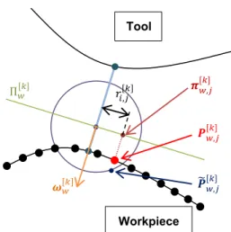
In order to displace the control points to mimic the shape of a sphere, a reference is needed. Let
Пi[k] be the plane that includes the centre of the sphere Ci[k] and that has ωi[k] as normal vector. Then,
for all the control points, Pi,j[k], j ∈{1,…,Ni[k]) and 𝑖 ∈
{𝑡, 𝑤}, the new position are computed as follows (figure 4):
𝑷7,C[>]= 𝑷7,C[>]+ 𝑓7,C[>] 𝑟7,C> . 𝝎7[>]
with 𝑓7,C> 𝑟7,C> = 𝑅7X− 𝑟7,C> X− 𝝎7>. (𝑷7,C[>]− 𝝅7,C>) and 𝑟7,C> = 𝝅7,C[>]− 𝑪7[>] , 𝝅7,C[>] being the projection of 𝑷7,C[>] on the plane Π7[>]
This process is repeated iteratively until no more craters can be inserted for the actual depth. Then, the tool is moved down along the 𝒛 axis with an increment of ∆( and the craters insertion process starts again. Tool Workpiece Π!["] 𝝎!["] 𝝅!,%["] 𝑷!,%["] 𝑟(,%["] 𝑷%!,%["]
Fig. 4. Plane Π#[>] Definition and a control point’s projection.
3.Experimental validation
As an initial evaluation of the new simulation process, two simple experiments were conducted on a Sarix SX-200 µEDM machine equipped with a wire dressing unit. A tungsten carbide rod, with a nominal diameter of 290µm was used as tool electrode. Ultra Fine Grained aluminium (Al1070) with an average grain size of 0.6μm was chosen as workpiece material to minimise material’s inhomogeneity while aiming at improving µEDM predictability, as suggested in [7].
Using the wire dressing unit, the tip of the tool electrode was machined flat for experiment 1 while for experiment 2 a curved shape was introduced (figure 5a). The electrodes were then used to erode the workpiece down to a 50µm depth. Machining parameters and results are shown in tables 1 and 2.Three simulations of Experiment 1 were then performed using different tolerances Tv to assess the
influence of the computational precision on roughness results (Table 3). The target volume 𝑉7 expected to be removed per crater was 279 µm3. Table 1
Machining parameters
Experiment 1 2
Energy level (index) 300 13
Voltage (V) 60 60 Current (index) 20 20 Time on (ms) 5 5 Table 2 Experimental results Experiment 1 2 Hole depth (µm) 50.8 50.2
Tool vertical wear (µm) 12.5 11.3
Roughness, Ra (µm) 1.27 0.82
Workpiece crater diameter (µm) 15 3 Workpiece crater depth (µm) 3 1
Table 3
Effect of volume removal precision on roughness
Tolerance (%) 10 5 1
Volume removed (µm3) 172058 169978 167586 Average volume (µm3)
removed per crater 286,76 283,30 279,31 Roughness, Ra (µm) 1,87 1,88 1,43 Table 4
Experiment and simulation results
Experimental tool vertical wear (µm) 11.3 Simulated tool vertical wear (µm) 11.2 Experimental roughness, Ra (µm) 0.82
Simulated roughness (µm) 0.87
Tool vertical wear deviation (%) 0.89
Roughness deviation (%) 6.09
b) a)
Fig.5. Experimental tool : a) before, b) after machining a)
b)
c)
Fig.6. Tool profiles. a) Experimentation b) Simulation c)
Profiles differences. black: simulation extra volume.
Table 3, clearly shows the significant influence of the tolerance level on the simulated roughness. Additionally it also highlights the importance of the measurements of the experimental craters and consequently the chosen volumes.
Following this, one simulation was performed for Experiment 2 to assess agreements in terms of geometry deformation due to tool wear, as well as achieved roughness. Based on the previous results, this simulation used a tolerance level Tv of 1%.
During the simulation process, a certain number of difficulties had to be managed with the displacement of control points. An evident case to avoid is displacing control points leading to self-intersecting geometries. This is often the case when dealing with the sides. As a result, the geometries must be taken into account when defining the warping vector. This will be optimised in the future.
Another issue linked to the surfaces’ parameterization occurred. A simple example highlighting this issue is to consider a scenario beginning with a flat surface. As it is being deformed, the control points’ displacements will lead to some areas of the surface having a smaller density of control points than others. A solution would be to regularly re-parameterize the surface to avoid this. It would however add to the already huge computation time. This will be further studied in the future.
Anyhow, the simulation results were very close to those of the experiment for the values of vertical
tool wear and roughness (table 4). Additionally, the tool’s profile can be compared with the simulated one (figure 6). It appears that the simulation does not lead to the dissymmetry present in the experimentation. This can be due to several factors that haven’t been included yet in the simulation, notably the influence of the dielectric flow and an eventual alignment error while machining the tool by wire EDM.
To validate fully the new simulation approach performance, further tests using a wider range of geometries are still required. However, these initial finding are encouraging and appear to demonstrate the viability of the method.
4.Conclusions
In order to overcome issues linked with the wear phenomenon in µEDM, it is important to be able to predict said wear. A viable method of simulation involving NURBS surfaces was presented. Although some discrepancies were found between experimental data and simulation results, those values remain acceptably close The importance of the measurement of experimental values was discussed. Another approach could be to use theoretical values for crater dimensions in lieu of the experimental ones. Efforts should also be put into preserving the surfaces’ parameterization as well as reducing the computational times.
Acknowledgements
This work was supported by the Engineering and Physical Sciences Research Council [EP/F056745/1, EP/J004901/1].
References
[1] S. Dhanik, S. S. Joshi Modeling of a single resistance capacitance pulse discharge in micro-electro discharge machining J. Manuf. Sci. Eng., Trans. ASME, 2005,
127, pp.759–767.
[2] G. Bissacco, H. N. Hansen, G. Tristo, J. Valentinčič. Feasibility of wear compensation in micro EDM milling based on discharge counting and discharge population characterization. CIRP ann., 2011, 60 (1), pp.231-234. [3] S. Bigot, A.Surleraux, G. Bissaco, J. Valenticic, A New
Modelling Framework for Die-Sinking Micro EDM, Proceedings of the 9th International Conference on Multi-Material Manufacture. 2012, pp.51-55.
[4] J. Kennedy, R. Eberhart. Particle Swarm Optimization. Proceedings of IEEE International Conference on Neural Networks IV. pp.1942–1948.
[5] L. Piegl, W. Tiller.The NURBS Book. Springer, 1996. [6] J.P. Pernot. Fully Free Form Deformation Features for
Aesthetic and Engineering Designs, Unpublished doctoral dissertation, Università di Genova & Institut National Polytechnique de Grenoble, 2004.
[7] S. Bigot, G. Bissacco, J. Valentinčič. Die-Sinking Micro EDM for Complex 3D Structuring - Research Directions. Int. Conf. on Multi-Material Micro Manufacture, Stuttgart, Germany, 8-9 November 2011.