HAL Id: hal-00407817
https://hal.archives-ouvertes.fr/hal-00407817
Submitted on 27 Jul 2009
HAL is a multi-disciplinary open access
archive for the deposit and dissemination of
sci-entific research documents, whether they are
pub-lished or not. The documents may come from
teaching and research institutions in France or
abroad, or from public or private research centers.
L’archive ouverte pluridisciplinaire HAL, est
destinée au dépôt et à la diffusion de documents
scientifiques de niveau recherche, publiés ou non,
émanant des établissements d’enseignement et de
recherche français ou étrangers, des laboratoires
publics ou privés.
Asymptotic Properties of Nonlinear Least Squares
Estimates in Stochastic Regression Models Over a Finite
Design Space. Application to Self-Tuning Optimisation
Luc Pronzato
To cite this version:
Luc Pronzato. Asymptotic Properties of Nonlinear Least Squares Estimates in Stochastic Regression
Models Over a Finite Design Space. Application to Self-Tuning Optimisation. 15th IFAC Symposium
on System Identification, Jun 2009, Saint Malo, France. pp.156-161. �hal-00407817�
Asymptotic Properties of Nonlinear Least
Squares Estimates in Stochastic Regression
Models Over a Finite Design Space.
Application to Self-Tuning Optimisation ?
Luc Pronzato∗
∗Laboratoire I3S, CNRS/Universit´e de Nice-Sophia Antipolis,
Bˆat Euclide, Les Algorithmes, 2000 route des lucioles, BP 121, 06903 Sophia Antipolis cedex, France (e-mail: [email protected])
Abstract: We present new conditions for the strong consistency and asymptotic normality of the least squares estimator in nonlinear stochastic models when the design variables vary in a finite set. The application to self-tuning optimisation is considered, with a simple adaptive strategy that guarantees simultaneously the convergence to the optimum and the strong consistency of the estimates of the model parameters. An illustrative example is presented.
Keywords: Optimal design of experiments; self-tuning optimisation; extremum seeking; penalized optimal design; sequential design; consistency; asymptotic normality.
1. INTRODUCTION
Consider a stochastic regression model with observations
Yk = η(xk, ¯θ) + εk, k = 1, 2 . . . (1)
where {εk} is a sequence of i.i.d. random variables with
IE(ε1) = 0 and IE(ε2
1) = σ2 < ∞, {xk} is a sequence
of design points in X ⊂ Rd and η(x, θ) is a known
function of x and parameter vector θ ∈ Θ, a compact subset of Rp, with ¯θ, the true unknown value of θ, such
that ¯θ ∈ int(Θ). We denote Fk the σ-field generated
by {Y1, . . . , Yk} and assume that xk is Fk−1 measurable.
This setup includes for instance the case of NARX models (nonlinear autoregressive models with exogeneous inputs) where Yk = η(Yk−1, . . . , Yk−a, uk−q, . . . , uk−q−b, ¯θ) + εk
where a, b ∈ N, q is the delay and uiis the input at stage i.
The unknown ¯θ will be estimated by Least Squares (LS)
and we denote Sn(θ) = n X k=1 [Yk− η(xk, θ)]2 and ˆθn
LS= arg minθ∈ΘSn(θ). We shall suppose that η(x, θ)
is continuously differentiable with respect to θ ∈ int(Θ) for all x ∈ X and denote fθ(x) = ∂η(x, θ)/∂θ and
M(ξ, θ) = Z
X
fθ(x)fθ>(x) ξ(dx) ,
the information matrix for parameters θ and design mea-sure ξ (a probability meamea-sure on X ). When ξ is the em-pirical measure ξk for x1, . . . , xk we get the information
matrix (normalized, per observation)
? This work was partly accomplished while the author was invited at
the Isaac Newton Institute for Mathematical Sciences, Cambridge, UK. The support of the Newton Institute and of CNRS are gratefully acknowledged. M(ξk, θ) = 1 k k X i=1 fθ(xi)fθ>(xi) .
In the case of a linear regression model where
η(x, θ) = f>(x)θ , ∀x ∈ X , θ ∈ Θ , (2) (so that M(ξ, θ) does not depend on θ), Lai and Wei [1982] show that the conditions
λmin[nM(ξn)]a.s.→ ∞ , n → ∞ (3)
{log λmax[nM(ξn)]}ρ/λmin[nM(ξn)]a.s.→ 0 , n → ∞ (4)
for some ρ > 1 are sufficient for the strong consistency of the LS estimator ˆθn
LS when {εk} in (1) is a martingale
difference sequence and supnIE(ε2
n|Fn−1) < ∞ a.s. The
case of nonlinear stochastic regression models is considered in [Lai, 1994], where sufficient conditions for strong consis-tency are given, which reduce to (3) and the Christopeit and Helmes [1980] condition,
λmax[nM(ξn)] = O{λρmin[nM(ξn)]} for some ρ ∈ (1, 2),(5)
in the case of a linear model.
This paper gives new sufficient conditions for the strong consistency of ˆθn
LS in nonlinear stochastic models. These
conditions, obtained under the assumption that {xk} lives
in a finite set, are much weaker than (3-4). The paper also
gives conditions under which √n M1/2(ξ
n, ˆθnLS)(ˆθLSn − ¯θ)
converges in distribution to a normal random variable
N (0, σ2I), with 0 and I respectively the p-dimensional null vector and identity matrix. This means that M(ξn, ˆθLSn )
can be used to characterize the asymptotic precision of the estimation of θ although the sequence of design points is stochastic. Conditions for strong consistency with a finite design space are given in Section 2 and conditions for asymptotic normality in Section 3. The application of
these results to self-tuning optimisation is considered in Section 4, where a comparison is made with the results in [Pronzato, 2000, Pronzato and Thierry, 2003]. A simple illustrative example is presented.
2. STRONG CONSISTENCY OF LS ESTIMATES WITH A FINITE DESIGN SPACE
Define Dn(θ, ¯θ) = n X k=1 [η(xk, θ) − η(xk, ¯θ)]2. (6)
Next theorem shows that the strong consistency of the LS estimator is a consequence of Dn(θ, ¯θ) tending to infinity
fast enough for θ 6= ¯θ. The fact that the design space X
is finite makes the required rate of increase for Dn(θ, ¯θ)
quite slow.
Theorem 1. Let {xi} be a design sequence on a finite set
X . If Dn(θ, ¯θ) given by (6) satisfies for all δ > 0 , · inf kθ−¯θk≥δDn(θ, ¯θ) ¸
/(log log n)a.s.→ ∞ , (7)
then ˆθn LS
a.s.
→ ¯θ as n → ∞. If Dn(θ, ¯θ) simply satisfies
for all δ > 0 , inf
kθ−¯θk≥δDn(θ, ¯θ) p → ∞ , (8) then ˆθn LS p → ¯θ as n → ∞.
The proof is given in [Pronzato, 2009] and is based on the following lemma from Wu [1981].
Lemma 2. If for any δ > 0
lim inf
n→∞ kθ−¯infθk≥δ[Sn(θ) − Sn(¯θ)] > 0 almost surely , (9)
then ˆθn LS a.s. → ¯θ as n → ∞. If for any δ > 0 Prob ½ inf kθ−¯θk≥δ[Sn(θ) − Sn(¯θ)] > 0 ¾ → 1 , n → ∞ , (10) then ˆθn LS p → ¯θ as n → ∞.
The condition [for all θ 6= ¯θ , Dn(θ, ¯θ) → ∞ as n → ∞]
is sufficient for the strong consistency of ˆθn
LS when the
parameter set Θ is finite, see Wu [1981]. From Theorem 1, when X is finite this condition is also sufficient for the weak consistency of ˆθn
LS without restriction on Θ. It is
proved in [Wu, 1981] to be necessary for the existence of a weakly consistent estimator of ¯θ in a regression model
when the errors εi are independent with a distribution
having a density ϕ(·) positive almost everywhere and ab-solutely continuous with respect to the Lebesgue measure and with finite Fisher information for location. Notice that a classical condition for strong consistency of LS estimates in nonlinear regression with non-random design is Dn(θ, ¯θ) = O(n) for θ 6= ¯θ, see e.g. Jennrich [1969],
which is much stronger than (7). Also note that (7) is much less restrictive than the conditions (3-4) for stochastic designs in linear models and than the Christopeit and Helmes [1980] condition (5).
3. ASYMPTOTIC NORMALITY OF LS ESTIMATES WITH A FINITE DESIGN SPACE
Under a fixed design, the information matrix can be con-sidered as a large sample approximation for the variance-covariance matrix of the estimator, thus allowing straight-forward statistical inference from the trial. The situation is more complicated for adaptive designs and has been intensively discussed in the literature. The property below gives a simple sufficient condition in the situation where the xk’s in (1) belong to a finite set. We use the following
regularity assumption for the model.
Hf: For all x in X , the components of fθ(x) are
con-tinuously differentiable with respect to θ in some open neighborhood of ¯θ.
Theorem 3. Assume that ˆθn
LS is strongly consistent, that
Hf is satisfied, that the design points belong to a finite set
X and that exists a sequence {Cn} of p × p deterministic
matrices such that C−1
n M1/2(ξn, ¯θ) → I, with lp n =
λmin(Cn) satisfying n1/4ln → ∞ and kˆθLSn − ¯θk/l2n
p → 0 as n → ∞. Then, ˆθn LSsatisfies √ n M1/2(ξn, ˆθnLS)(ˆθLSn − ¯θ) d → ω ∼ N (0, σ2I) (11) as n → ∞.
One may notice that, compared to Wu [1981], we do not require that (n/τn)M(ξn, ¯θ) tends to a positive definite
matrix for some τn → ∞ and, compared to Lai and Wei
[1982], Lai [1994], we do not require the existence of high-order derivatives of η(x, θ) w.r.t. θ. On the other hand, we need that λmin(Cn) decreases more slowly than n−1/4.
4. APPLICATION TO SELF-TUNING OPTIMISATION
4.1 Problem statement
We consider a self-tuning optimisation problem where one wishes to minimize some function φ(x, ¯θ) with respect to
x, the unknown parameters ¯θ being estimated from the
observations in the model (1). One may have φ(·, ·) = η(·, ·) but this is not mandatory. In particular, less regularity is required for φ(x, ·) than for η(x, ·) and we shall only use the following assumptions on φ.
Hφ-(i): φ(x, θ) is bounded for below and above for any
x ∈ X and θ ∈ Θ.
Hφ-(ii): For all x ∈ X , φ(x, θ) is a continuous function of
θ in the interior of Θ.
Hφ-(iii): φ(x, ¯θ) has a unique global minimizer x∗= x∗(¯θ):
∀β > 0, ∃² > 0 such that φ(x, ¯θ) < φ(x∗, ¯θ) + ² implies
kx − x∗k < β.
Note that compared to methods based on local gradient approximations, see, e.g. [Manzie and Krsti´c, 2007], the method is not restricted to a neighborhood of a local minimum of φ(x, ¯θ). On the other hand, we shall assume
that x belongs to a finite space and φ(x, θ) must have a known parametric form.
When the problem is to estimate x∗, one can resort to
order to optimize a criterion that measures the precision of the estimation of θ in (1). For instance, one may use a nominal value θ0 for θ, construct a D-optimal design measure ξ∗
D(θ0) on X maximizing log det M(ξ, θ0) and
choose xk’s such that their empirical measure approaches
ξ∗
D(θ0). Alternatively, one may relate the design criterion
to the estimation of x∗(θ), see, e.g., [Chaloner, 1989,
Pronzato and Walter, 1993].
In self-tuning optimisation, the design points form a se-quence of control variables for the objective of minimizing P
iφ(xi, ¯θ). The trivial optimum solution xi = x∗(¯θ) for
all i is not feasible since ¯θ is unknown, hence the dual
aspect of the control: minimize the objective, help esti-mate θ. A naive approach (Forced-Certainty-Equivalence control) consists in replacing the unknown ¯θ by its current
estimated value at stage k, that is, xk+1= x∗(ˆθkLS).
How-ever, this does not provide enough excitation to estimate
θ consistently, see Bozin and Zarrop [1991] for a detailed
analysis of the special case φ(x, θ) = η(x, θ) = θ1x + θ2x2. Here we shall consider the same approach as in [Pronzato, 2000, Pronzato and Thierry, 2003] and use
xn+1= arg min x∈X n φ(x, ˆθLSn ) −αnfθˆ>n LS(x)M −1(ξ n, ˆθLSn )fˆθn LS(x) o , (12) with αn > 0; that is, to the current objective φ(x, ˆθnLS),
to be minimized with respect to x, we add a penalty for poor estimation, −αnfθˆ>n
LS
(x)M−1(ξ
n, ˆθnLS)fθˆn
LS(x) (note
that xn+1 is Fn-measurable). Iterations of the similar
type can be used to generate an optimal design under a cost-constraint, the cost of an observation at the design point x for parameters θ being measured by φ(x, θ), see [Pronzato, 2008]. See also ˚Astr¨om and Wittenmark [1989]. The results in Section 4.2 indicate that when X is finite and the sequence of penalty coefficients αn decreases
slowly enough, the LS estimator ˆθn
LSis strongly consistent.
When ˆθn
LSis frozen to a fixed value θ and αn≡ α constant,
the iteration (12) corresponds to one step of a steepest descent vertex-direction algorithm for the minimisation of R
Xφ(x, θ) ξ(dx) − α log det M(ξ, θ), with step-length 1/n
at stage n. Convergence of the empirical measure ξn to
an optimal design measure is proved in [Pronzato, 2000] using an argument developed in [Wu and Wynn, 1978]. It is also shown in the same reference thatRXφ(x, θ) ξn(dx) →
minx∈Xφ(x, θ) as n → ∞ when αn decreases to zero and
the sequence {nαn} increases to infinity. If, moreover, Hφ
-(iii) is satisfied then ξn → δw x∗(θ) (weak convergence of
probability measures), with δx the delta measure at x. Those results do not require X to be finite.
The fact that the parameters are estimated in (12) makes the proof of convergence a much more complicated issue. In the case of the linear regression model (2) it is shown in [Pronzato, 2000] that if {αn} is such that αnlog n
decreases to zero and nαn/(log n)1+δ increases to infinity
for some δ > 0, then RXφ(x, ¯θ) ξn(dx) a.s.→ minx∈Xφ(x, ¯θ) (and ξn→ δw x∗(¯θ)a.s. if Hφ-(iii) is satisfied). Using Bayesian
imbedding, the same properties are shown to hold in [Pronzato and Thierry, 2003] under the weaker conditions
αn → 0 and nαn → ∞ (however, the almost sure
convergence then concerns the product measure µ×Q with
µ the prior measure for θ and Q the probability measure
induced by {εk}). To the best of our knowledge, no similar
result exists for nonlinear regression models.
When φ(x, θ) = 0 for all x the iteration (12) becomes xn+1= arg max x∈Xf > ˆ θn LS(x)M −1(ξ n, ˆθLSn )fˆθn LS(x) , (13)
which corresponds to one step in the sequential construc-tion of a D-optimal design. Even for this particular situ-ation, and although this method is widely used, very few asymptotic results are available: the developments in [Ford and Silvey, 1980, Wu, 1985, M¨uller and P¨otscher, 1992] only concern a particular example; [Hu, 1998] is specific of Bayesian estimation by posterior mean and does not use a fully sequential design of the form (13); Lai [1994] and Chaudhuri and Mykland [1995] require the introduction of a subsequence of non-adaptive design points to ensure consistency of the estimator and Chaudhuri and Mykland [1993] require that the size of the initial experiment (non-adaptive) grows with the increase in size of the total experiment. Intuitively, the almost sure convergence of ˆθn
LS
to some ˆθ∞would be enough to imply the convergence of
ξn to a D-optimal design measure for ˆθ∞ and, conversely,
convergence of ξn to a design ξ∞ such that M(ξ∞, θ) is
non-singular for any θ would be enough in general to make the estimator consistent. It is thus the interplay between estimation and design iterations (which implies that each design point depends on previous observations) that creates difficulties. As the results below will show, those difficulties disappear when X is a finite set. Notice that the assumption that X is finite is seldom limitative since practical considerations often impose such a restric-tion on possible choices for the design points; this can be contrasted with the much less natural assumption that would consist in considering the feasible parameter set as finite, see, e.g., Caines [1975].
The results below rely on simple arguments based on three ideas. First, we consider iterations of the form
xn+1= arg min x∈X n φ(x, ˆθn) −αnfθ>ˆn(x)M −1(ξ n, ˆθn)fˆθn(x) o , (14)
where {ˆθn} is taken as any sequence of vectors in Θ.
The asymptotic design properties obtained within this framework thus also apply when ˆθn corresponds to ˆθn
LS.
Second, when X is finite we obtain a lower bound on the sampling rate of a subset of points of X associated with a nonsingular information matrix. Third, we can show that this bound guarantees the strong consistency of ˆθn
LS.
With a few additional technicalities, this yields almost sure convergence results for the adaptive designs constructed via (12).
4.2 Asymptotic properties of LS estimates and designs
We shall use the following assumptions on X . HX-(i): X is finite, X = {x(1), x(2), . . . , x(K)}.
HX-(ii): infθ∈Θλmin hPK
i=1fθ(x(i))fθ>(x(i))
i
HX-(iii): For all δ > 0 there exists ²(δ) > 0 such that for
any subset {i1, . . . , ip} of distinct elements of {1, . . . , K},
inf kθ−¯θk≥δ p X j=1 [η(x(ij), θ) − η(x(ij), ¯θ)]2> ²(δ) .
HX-(iv): For any subset {i1, . . . , ip} of distinct elements
of {1, . . . , K}, λmin p X j=1 f¯θ(x(ij))fθ>¯(x(ij)) ≥ ¯γ > 0 .
The case of sequential D-optimal design, correspond-ing to the iterations (13), is considered in [Pronzato, 2009]. When αn → α > 0 (n → ∞) in (12), the
results are similar to those in [Pronzato, 2009] and ˆ θn LS a.s. → ¯θ, M(ξn, ˆθnLS) a.s. → M(ξ∗, ¯θ) with ξ∗ minimizing R
Xφ(x, ¯θ) ξ(dx) − α log det M(ξ, ¯θ). One can take Cn =
M1/2(ξ∗, ¯θ) for all n in Theorem 3 and ˆθn
LS is
asymptoti-cally normal.
The situation is more complicated when the sequence {αn}
in (12,14) satisfies the following:
Hα-(i): {αn} is a non-increasing positive sequence tending
to zero as n → ∞,
the situation considered in the rest of the paper. We then obtain the following lower bound on the sampling rate of nonsingular designs.
Lemma 4. Let {ˆθn} be an arbitrary sequence in Θ used to
generate design points according to (14) in a design space satisfying HX-(i), HX-(ii), with an initialisation such that
M(ξn, θ) is non-singular for all θ in Θ and all n ≥ p. Let
rn,i = rn(x(i)) denote the number of times x(i) appears
in the sequence x1, . . . , xn, i = 1, . . . , K, and consider the
associated order statistics rn,1:K ≥ rn,2:K ≥ · · · ≥ rn,K:K.
Define
q∗= max{j : ∃β > 0| lim inf
n→∞ rn,j:K/(nαn) > β} .
Then, Hφ-(i) and Hα-(i) imply q∗ ≥ p with probability
one.
For any sequence {ˆθn} used in (14), the conditions of
Lemma 4 ensure the existence of N1 and β > 0 such that
rn,j:K > βnαn for all n > N1 and all j = 1, . . . , p. Under
the additional assumption HX-(iii) we thus obtain that
Dn(θ, ¯θ) given by (6) satisfies
1
log log n kθ−¯infθk≥δDn(θ, ¯θ) >
βnαn²(δ)
log log n , n > N1. Therefore, if nαn/ log log n → ∞ as n → ∞, ˆθLSn
a.s.
→ ¯θ
from Theorem 1. Since this holds for any sequence {ˆθn} in
Θ, it is true in particular when ˆθn
LS is substituted for ˆθn
in (14). It thus holds for (12). Using the following assumption
Hα-(ii): the sequence {αn} is such that nαn is
non-decreasing with nαn/ log log n → ∞ as n → ∞;
in complement of Hα-(i), one can show that the adaptive
design algorithm (12) is such that {xn} tends to
accumu-late at the point of minimum cost for ¯θ.
Theorem 5. Suppose that in the regression model (1)
the design points for n > p are generated sequentially according to (12), where αn satisfies Hα-(i) and Hα-(ii).
Suppose, moreover, that the first p design points are such that the information matrix is nonsingular for any
θ ∈ Θ. Then, under HX-(i-iv), Hφ-(i) and Hφ-(ii) we have
ˆ θn LS a.s. → ¯θ and Z X φ(x, ¯θ) ξn(dx)a.s.→ min x∈Xφ(x, ¯θ) , n → ∞ . (15) If, moreover, Hφ-(iii) is satisfied, then
ξn → δw x∗(¯θ) almost surely , n → ∞ . (16)
Remark 6. Notice that the condition on the rate of
de-crease of {αn} in Theorem 5 is weaker than in [Pronzato,
2000] although the model is nonlinear. Also note that using a penalty for poor estimation of the form
−Cdet h fˆθn LS(x)f > ˆ θn LS (x) +Pnk=1fθˆn LS(xk)f > ˆ θn LS (xk) i dethPnk=1fˆθn LS(xk)f > ˆ θn LS (xk) i , C > 0,
as suggested in [˚Astr¨om and Wittenmark, 1989] is equiv-alent to taking αn = C/n in (12), which does not satisfy
Hα-(ii) and therefore does not guarantee the strong
con-sistency of the LS estimates.
Remark 7. The property (16) does not imply that the
xk’s generated by (12) converge to x∗(¯θ). However, the
following property is proved in [Pronzato, 2008]. Suppose that X is obtained by the discretization of a compact set
X0 and define x = arg min
x∈X0φ(x, ¯θ) and, for any design
measure ξ on X0, ∆¯ θ(ξ) =
R
X0φ(x, ¯θ) ξ(dx) − φ(x, ¯θ).
Suppose that there exist designs measures ξα on X0 such
that ∆¯θ(ξα) ≥ pα and for all ² > 0
lim sup α→0+ sup x∈X0, kx−xk>² 2∆¯θ(ξα) [fθ>¯(x)M−1(ξα, ¯θ)fθ¯(x)] φ(x, ¯θ) − φ(x, ¯θ) < 1.
Then the supporting points of an optimal design measure minimizing RX0φ(x, ¯θ) ξ(dx) − α log det M(ξ, ¯θ) converge
to x as α → 0+, and, under the conditions of Theorem 5, the design sequence {xn} on X will concentrate around
x∗(¯θ) as n → ∞.
Remark 8. Under the conditions of Theorem 5, there exist N0 and β > 0 such that, for all n > N0, λmin[M(ξn, ¯θ)] >
β¯γαn, with ¯γ as in HX-(iv). The asymptotic normality of
ˆ
θn
LS is ensured if one can exhibit a sequence {Cn}
satis-fying the conditions of Theorem 3. For λmin(Cn) ∼ α1/2n
we then obtain that imposing the condition n1/3α
n → ∞
on the decrease rate of αn would be enough. A possible
construction is based on the matrix M1/2(ν
n, ¯θ) obtained
when ¯θ is substituted for ˆθn
LSin the iterations (12).
How-ever, it remains to be proved that M−1(ν
n, ¯θ)M(ξn, ¯θ)
p
→
I, which is not obvious (notice that the sequence {ˆθn LS}
becomes highly correlated as n increases).
Remark 9. When the function to be minimized is the
model response itself and, moreover, is linear with respect to θ, one can construct analytical approximate solutions for the self-tuning optimizer over a finite horizon N when using a Bayesian approach. In particular, one of the constructions proposed in [Pronzato and Thierry, 2003] is shown to be within O(σ4) of the optimal solution of
0 50 100 150 200 250 300 350 400 450 500 −1 −0.8 −0.6 −0.4 −0.2 0 0.2 0.4 0.6 0.8 1 n xn
Fig. 1. A typical sequence {xn}, αn= (log n)−4
the self-tuning optimizer problem (the latter being not computable, it corresponds to the solution of a stochastic dynamic programming problem).
4.3 Example
We take η(x, θ) = θ1θ2θ3+ θ2x + θ3(1 + θ12) x2 + θ21x3,
φ(x, θ) = θ2 + θ1x2 + θ2θ3x4, with x ∈ [−1, 1] and
θ = (θ1, θ2, θ3)>∈ R. One can easily check that the model is structurally globally identifiable so that, if the sequence
{xk} is rich enough, the LS estimator is unique and θ
can be estimated consistently. For the true value ¯θ of the
parameters we take ¯θ = (0, 1, 1)> which gives f¯ θ(x) =
(1, x, x2)> and φ(x, ¯θ) = 1 + x4. The optimal design
ξ∗(α) on X0 = [−1, 1] that minimizes R
X0φ(x, ¯θ) ξ(dx) −
α log det M(ξ, ¯θ) can be constructed analytically for any α, see [Pronzato, 2008]. For α < 2/9, the support points
are −√3(α/2)1/4, 0,√3(α/2)1/4, with respective weights 1/6, 2/3, 1/6, showing that ξ∗(α) concentrates around 0 =
arg minx∈X0φ(x, ¯θ) as α tends to zero.
Figure 1 shows a typical sequence {xn} generated by (12)
for n ≥ 3 when σ = 1, x1 = −1, x2 = 0, x3 = 1, αn =
(log n)−4 and X consists of 201 points regularly spaced
in [−1, 1]. The design points tend to concentrate around
x∗(¯θ) = 0 as n increases. This is due to the fact that
φ(x, ¯θ) is sufficiently flat around x∗(¯θ). The situation can
be much different for other functions φ, see for instance the examples in [Pronzato, 2000, Pronzato and Thierry, 2003] where (16) is satisfied but design points are continuously generated far from x∗(¯θ) (although less and less often as
n increases).
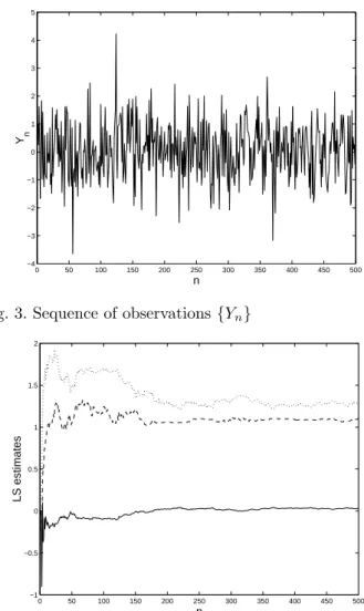
Figure 2 presents the corresponding sequence {φ(xn, ¯θ)},
showing that convergence to the minimum value 1 is fast despite the model is nonlinear and the observations are very noisy, see Figure 3 for a plot of the sequence {Yn}.
The evolution of the parameter estimates ˆθn
LSis presented
in Figure 4.
4.4 A concluding remark on the difficulties raised by dynamical systems
Compared to [Choi et al., 2002] where a periodic dis-turbance of magnitude α plays the role of a persistently
0 50 100 150 200 250 300 350 400 450 500 1 1.001 1.002 1.003 1.004 1.005 1.006 1.007 1.008 1.009 n φ (xn , θ )
Fig. 2. Corresponding sequence {φ(xn, ¯θ)}, n ≥ 8
0 50 100 150 200 250 300 350 400 450 500 −4 −3 −2 −1 0 1 2 3 4 5 n Yn
Fig. 3. Sequence of observations {Yn}
0 50 100 150 200 250 300 350 400 450 500 −1 −0.5 0 0.5 1 1.5 2 n LS estimates Fig. 4. LS estimates ˆθn
LS (solid line for θ1, dashed-line for
θ2and dots for θ3)
exciting input signal and the output converges to a neigh-borhood O(α2) of the optimum, iterations of the form (12) guarantee exact asymptotic convergence to the optimum when the excitation provided by the penalty for poor esti-mation vanishes slowly enough, see Theorem 5. However, (12) assumes that xn+1can be chosen freely in a given X
that does not depend on xn; that is, it implicitly assumes
fact that xn+1depends on ˆθLSn that introduces a dynamic
feedback), whereas Choi et al. [2002] consider self-tuning optimisation of a dynamic discrete-time system. (See also Krsti´c [2000], Krsti´c and Wang [2000] for continuous-time dynamic systems). Within the setup of Choi et al. [2002], it means that we need to observe the input of the static nonlinearity. This is a rather severe limitation, but one that seems difficult to overcome.
To illustrate the problem, consider the classical algorithm for the sequential construction of a D-optimal design with iterations of the form (13), see [Wynn, 1970]. Take the linear model η(x, θ) = θ1x + θ2x2, so that fθ(x) = f (x) =
(x, x2)>, and suppose that x
n may only vary within the
interval [−1, 1] by increments of ±δ in one iteration (so that xn+1= xn+1(un) = max{−1, min{1, xn+ un}} with
un ∈ {−δ, 0, δ}), with 1/δ integer. Also suppose that
M(ξn0) is non singular for some n0 and that xn0 = mδ ∈
[0, 1] with m a strictly positive integer. One can easily check that the iterations
un= arg max u∈{−δ,0,δ}f
>(x
n+ un)M−1(ξn)f (xn+ un)
for n ≥ n0 do not yield convergence to the D-optimal design measure ξ∗
D (which allocates weights 1/2 at the
extreme points ±1). Indeed, negative values for xn can
only be reached if xk = 0 is selected for some k ≥ n0, which
is impossible since f (0) = 0. Other types of iterations, perhaps less myopic than (12) and (13) which only look one step-ahead, should thus be considered for general dynamic systems.
5. CONCLUSIONS
Self-tuning optimisation has been considered through an approach based on sequential penalized optimal design. Simple conditions have been given that guarantee the strong consistency of the LS estimator in this context of sequentially determined control variables, under the assumption that they belong to a finite set and that the penalty for poor estimation does not decrease too fast.
REFERENCES
K.J. ˚Astr¨om and B. Wittenmark. Adaptive Control.
Addison Wesley, 1989.
A.S. Bozin and M.B. Zarrop. Self tuning optimizer — convergence and robustness properties. In Proc. 1st
European Control Conf., pages 672–677, Grenoble, July
1991.
P.E. Caines. A note on the consistency of maximum likeli-hood estimates for finite families of stochastic processes.
Annals of Statistics, 3(2):539–546, 1975.
K. Chaloner. Bayesian design for estimating the turning point of a quadratic regression. Commun. Statist.-Theory Meth., 18(4):1385–1400, 1989.
P. Chaudhuri and P.A. Mykland. Nonlinear experiments: optimal design and inference based likelihood. Journal
of the American Statistical Association, 88(422):538–
546, 1993.
P. Chaudhuri and P.A. Mykland. On efficiently designing of nonlinear experiments. Statistica Sinica, 5:421–440, 1995.
J.-Y. Choi, M. Krsti´c, K.B. Ariyur, and J.S. Lee. Extremum seeking control for discrete-time systems.
IEEE Transactions on Automatic Control, 47(2):318–
323, 2002.
N. Christopeit and K. Helmes. Strong consistency of least squares estimators in linear regression models. Annals
of Statistics, 8:778–788, 1980.
I. Ford and S.D. Silvey. A sequentially constructed design for estimating a nonlinear parametric function.
Biometrika, 67(2):381–388, 1980.
I. Hu. On sequential designs in nonlinear problems.
Biometrika, 85(2):496–503, 1998.
R.I. Jennrich. Asymptotic properties of nonlinear least squares estimation. Annals of Math. Stat., 40:633–643, 1969.
M. Krsti´c. Performance improvement and limitations in extremum seeking control. System & Control Letters, 39:313–326, 2000.
M. Krsti´c and H.-H. Wang. Stability of extremum seeking feedback for general nonlinear dynamic systems.
Auto-matica, 36:595–601, 2000.
T.L. Lai. Asymptotic properties of nonlinear least squares estimates in stochastic regression models. Annals of
Statistics, 22(4):1917–1930, 1994.
T.L. Lai and C.Z. Wei. Least squares estimates in stochas-tic regression models with applications to identification and control of dynamic systems. Annals of Statistics, 10 (1):154–166, 1982.
C. Manzie and M. Krsti´c. Discrete time extremum seeking using stochastic perturbations. In Proceedings of the
46th Conf. on Decision and Control, pages 3096–3101,
New Orleans, Dec. 2007.
W.G. M¨uller and B.M. P¨otscher. Batch sequential design for a nonlinear estimation problem. In V.V. Fedorov, W.G. M¨uller, and I.N. Vuchkov, editors, Model-Oriented
Data Analysis II, Proceedings 2nd IIASA Workshop, St Kyrik (Bulgaria), May 1990, pages 77–87. Physica
Verlag, Heidelberg, 1992.
L. Pronzato. One-step ahead adaptive D-optimal de-sign on a finite dede-sign space is asymptotically optimal.
Metrika, 2009. to appear.
L. Pronzato. Penalized optimal designs for dose-finding. Technical Report I3S/RR-2008-18-FR, Laboratoire I3S, CNRS–Universit´e de Nice-Sophia Antipolis, 06903 Sophia Antipolis, France, 2008. http://www.i3s.unice.fr/ mh/RR/rapports.html. L. Pronzato. Adaptive optimisation and D-optimum
experimental design. Annals of Statistics, 28(6):1743– 1761, 2000.
L. Pronzato and E. Thierry. Sequential experimental design and response optimisation. Statistical Methods
and Applications, 11(3):277–292, 2003.
L. Pronzato and E. Walter. Experimental design for estimating the optimum point in a response surface.
Acta Applicandae Mathematicae, 33:45–68, 1993.
C.F.J. Wu. Asymptotic theory of nonlinear least squares estimation. Annals of Statistics, 9(3):501–513, 1981. C.F.J. Wu. Asymptotic inference from sequential design in
a nonlinear situation. Biometrika, 72(3):553–558, 1985. C.F.J. Wu and H.P. Wynn. The convergence of general step–length algorithms for regular optimum design cri-teria. Annals of Statistics, 6(6):1273–1285, 1978. H.P. Wynn. The sequential generation of D-optimum
experimental designs. Annals of Math. Stat., 41:1655– 1664, 1970.