is an open access repository that collects the work of Arts et Métiers Institute of
Technology researchers and makes it freely available over the web where possible.
This is an author-deposited version published in: https://sam.ensam.eu Handle ID: .http://hdl.handle.net/10985/6819
To cite this version :
Olivier COUTIER-DELGOSHA, Antoine DAZIN, Guy CAIGNAERT, Gérard BOIS - Analysis of Cavitation Instabilities in a Four-Blade Inducer - Analysis of Cavitation Instabilities in a Four-Blade Inducer - Vol. 2012, n°ID 213907, p.1-11 - 2012
Any correspondence concerning this service should be sent to the repository Administrator : [email protected]
Volume 2012, Article ID 213907,11pages doi:10.1155/2012/213907
Research Article
Analysis of Cavitation Instabilities in a Four-Blade Inducer
O. Coutier-Delgosha, A. Dazin, G. Caignaert, and G. Bois
Arts et Metiers ParisTech/LML Laboratory, 8 boulevard Louis XIV, 59046 Lille Cedex, France
Correspondence should be addressed to O. Coutier-Delgosha,[email protected]
Received 26 December 2011; Accepted 18 April 2012 Academic Editor: Meinhard Taher Schobeiri
Copyright © 2012 O. Coutier-Delgosha et al. This is an open access article distributed under the Creative Commons Attribution License, which permits unrestricted use, distribution, and reproduction in any medium, provided the original work is properly cited.
The cavitating behavior of a four-blade inducer tested in the LML laboratory large test facility is considered in the present paper. Experimental investigations based on unsteady pressure measurements and records from a six-component balance mounted on the inducer shaft are performed. Spectral analysis of the signals enables to detect several characteristic frequencies related to unbalanced two-phase flow patterns. The objective of the present paper is the understanding of the physical phenomena associated to these frequencies. Therefore, wavelet decomposition, flow visualizations, and direct analysis of the high-frequency force, moment, and pressure signals are applied. Results at nominal flow rate only are considered. Not only classical unbalanced cavitation patterns, but also unexpected flow organizations are discussed.
1. Introduction
Rocket engine turbopump inducers are designed to operate in cavitating conditions, because of the low pressure of LH2 and LOX in the tanks. However, development of cavitation must be controlled to avoid any reduction of the inducer per-formance. Attention is also focused on instabilities associated with cavitation, since they are responsible for unbalanced flow pattern that compromise the rotor equilibrium. Self-oscillation of the sheet cavities on the blades may also generate problematic pressure fluctuations at the inducer outlet.
The understanding of these different unsteady flow behaviors has not been completed, yet, although significant progress has been achieved in the last decades. Experimental investigations of the behavior of various inducers, character-ized by a blade number varying usually between 2 and 5, have been conducted for example in Pisa University (Italy) in collaboration with Avio, in Arts et Metiers ParisTech and CREMHyG (France) in collaboration with SNECMA Moteurs, and in Osaka University (Japan) by Tsujimoto and colleagues in cooperation with the JAXA program. In these different studies, several recurrent unstable behaviors have been identified: (i) rotating cavitation is characterized by a nonsymmetrical two-phase flow pattern, which rotates
faster or slower than the inducer, leading to so-called super-synchronous or subsynchronous regimes, respectively. Rotation speed in the inducer rotating frame is generally low, leading in the absolute frame to frequencies close to the inducer rotation one. Such phenomenon, which leads to significant radial forces, has been detected in nearly all tested inducers [1–3] (Tsujimoto et al. 1997). (ii) A surge mode oscillation characterized by a global pulsation of the vapor areas at low frequency: such oscillations have been investigated in simpler configurations of 2D Venturi profiles or 2D foil sections in cavitation tunnels and analyzed in details by many authors [4–7]. (iii) Rotating stall in backflow vortices: such behavior has been identified by Tsujimoto and colleagues [8] in the case of cavitation clouds extending upstream from the inducer inlet. It basically consists in a slow rotation of this detached cavitation, at frequency that depends on the number of vortices.
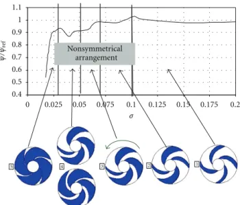
The occurrence of these different flow patterns strongly depends on the cavitation development in the machine. A typical sketch in the case of a four-blade inducer is given for example in Figure1.
At cavitation inception, only a steady and balanced flow pattern with one short attached cavity on each blade is observed from flow visualizations. When cavitation param-eter is slightly decreased, a steady and alternate cavitating
Nonsymmetrical arrangement 0 5 4 3 2 1 0.025 0.05 0.075 0.1 0.125 0.15 0.175 0.2 1.1 1 0.9 0.8 0.7 0.6 0.5 0.4 ψ /ψre f σ
Figure 1: Sketches of cavitation patterns and performance evolu-tion as the cavitaevolu-tion number decreases in a four-blade inducer [9].
configuration appears with alternatively one short and one long cavity. For a lower cavitation parameter, just above breakdown, rotating cavitation can be identified: unbalanced attached cavities are observed in the different channels, their distribution rotating faster than the inducer. Finally near the breakdown of the inducer, a steady and balanced flow pattern with fully developed cavitation is observed.
More recently, supplementary unstable flow patterns have been identified in particular configurations: (i) higher-order rotating cavitation has been reported first by Fujii et al. [10], from Osaka University, in the case of a three-blade inducer. Frequency related to this phenomenon is 5
frefin the absolute frame. (ii) Higher-order cavitation surge:
this axial instability has been found by the Osaka Team at frequency 5 fref, and also by researchers from Pisa University
at frequencies 4.4 frefand 6.6 frefin the case of a two-blade
inducer. In both cases, the phenomenon was detected at high flow coefficient.
These instabilities induce some strong radial forces that may perturb the rotor balance, and important pressure fluc-tuations in the lines. They must be quantified and controlled to avoid any major effect on the global pump behavior. Their detection is usually based, in all aforementioned references, on pressure transducers mounted on the inducer shroud at several angles in the same section. The analysis of the phase difference between the transducers enables to distinguish axial instabilities (characterized by zero-phase difference) from rotating cavitation (where a phase difference equal to the angle difference is obtained).
As can be seen, the physical characterization of the flow instabilities related to cavitation is still weak, which explains that only a few attempts have been performed to explain inception and mechanisms of rotating cavitation [11,
12]. Yoshida and colleagues state that inception of unstable behaviours is mainly governed by the sheet cavity length Lc.
Sheet cavities longer than the cascade throat remain equal
20 cm
Figure 2: Inducer geometry.
because they are fully constrained by the adjacent blade. In opposition, sheet cavities that do not reach the cascade throat (0.8 < Lc/h < 1) are characterized by a degree of freedom,
which may lead to unstable cavitation such as synchronous nonsymmetrical flow patterns. However, no consensus is presently obtained concerning too the mechanisms that are responsible for the inception of unbalanced flow patterns as the ones that control the successive synchronous and non-synchronous regimes that are usually observed in inducers.
Conversely, several studies have been conducted to investigate the effects of the inducer design on its unsteady behavior: it has been found, for example, that the shape of the hub [13], of the leading edge [14], (Bakir et al. 2002), and even of the casing [15] have significant influence on cavitation instabilities. The effects of unequal spacing of the blades have been also investigated by numerical simulations [16]. All inducers have been usually manufactured with one to 4 blades in the inlet section.
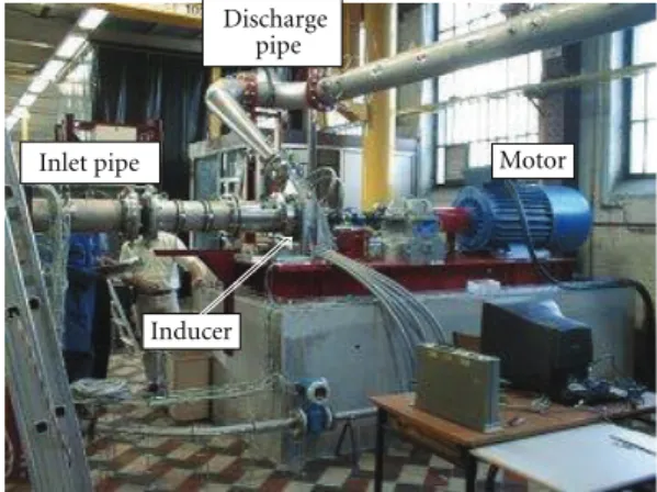
In the present paper, the cavitating behaviour of a four-blade inducer (Figure 2) is investigated. Experiments have been performed in the large test facility of ENSAM Lille, with the collaboration of the CNES (French Space Agency) and SNECMA Moteurs. Although a large range of mass flow rates, inlet pressures, and rotation speeds have been tested, attention is focused presently on a few hydrodynamic conditions only, at nominal mass flow rate Qnand reference
rotation speed Nref. The successive flow instabilities, which
are encountered when the inlet pressure is progressively decreased, are analysed in details, in order to improve their characterization and physical understanding. Original force measurements performed with a balance mounted on the inducer shaft, associated with unsteady pressure measurements on the inducer shroud, enable to obtain data both in the absolute and inducer rotating frame, which enriches the analysis of the results.
Note that all results presented in the paper are dimen-sionless for reasons of confidentiality. So, the “+” indicates that each variable V+ is V/V
0where V0is a reference value
Inducer
Motor Discharge
pipe
Inlet pipe
Figure 3: General view of the LML large test facility.
2. Experimental Setup
2.1. Test Facility. The LML laboratory large test facility
devoted to the study of axial pumps in cavitating conditions has been used for the experiments. This two-stairs facility is equipped with a 200 kW motor that enables to reach an inducer rotation speed of 6000 rpm. The device upstairs (Figure3) is mainly composed of the inducer to be tested and a stator downstream from the inducer that conducts the flow towards the discharge pipe. The inlet and discharge pipes are connected to two tanks. A free surface is maintained in the upstream one, so that the pressure can be controlled in the installation, from about 0.1 bars up to 16 bars. A part
Qs of the volume flow rate is taken at the inducer outlet
for the axial equilibrium device, and then reinjected in the upstream tank. Downstairs are located two large resorption tanks used for the extraction of dissolved gas, a variable head loss device that enables to control the flow rate, and the vacuum pump used to decrease the pressure in the inlet tank. A heat exchanger is also connected to the facility to control the water temperature.
2.2. Acquisition Device. The inducer test section is equipped
with a large variety of sensors devoted either to the charac-terization of steady flow properties, or to the analysis of the flow unsteady fluctuations.
Concerning steady flow properties, the torque Mx and
the rotation speed N are measured with a Torquemaster TM213 torque meter, while a Rosemount AP6 pressure transducer (range 0–6 bars) is used for the inlet pressure Pi. A
Rosemount DP7E22 differential pressure transducer (range 0–16 bars) connected between Pi and Pd is used to obtain
directly the elevation ∆P. The main flow rate Qm and the
recirculating one Qs are measured with Endress + Hauser
electromagnetic flow meters. The motor shaft rotation speed is also controlled with a photoelectric cell.
Temperature measurements are performed on the upstream and downstream bearings of the inducer shaft, to control their increase at high rotation speed, and the water temperature is measured to regulate the heat exchanger operation so that a 25◦C temperature is maintained in the
flow. The torque Mxand the rotation speed N are acquired
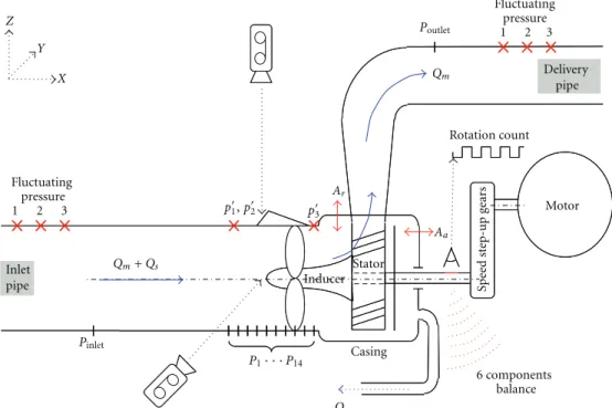
at frequency 100 Hz during 10 s, while all other signals are recorded at frequency 40 Hz during 140 s. From these records, mean and RMS values of the signals are calculated for each investigated flow condition. Note that the inlet and outlet pressures are measured in the inlet and delivery pipes more than one meter upstream and downstream from the inducer, so the calculated pressure head includes the head losses between the two pressure taps, including the one in the stator and in the downstream 90◦bends that can be seen
in Figure4.
Absolute uncertainties on the mean flow characteristics are 0.5% of Qreffor Qm, 0.05% of Qreffor Qs, 0.25% of Nref
for N, 2% of the noncavitating torque value for Mx, and
0.2% of the measurement range for the upstream pressure and ∆P. Precision regarding the cavitation number and the head, torque, and flow rate coefficients depend on the flow conditions and will be indicated in the figures hereafter.
Unsteady flow properties are investigated with nine Kistler 701A piezo-electric pressure transducers (Figure4): six of them are located in the upstream and delivery pipes, two other ones (P"
1 and P2") are located at the inlet of the
inducer test section, and the last one P"
3 is between the
inducer and the stator. All transducers are mounted flush to the internal pipe wall. Four accelerometers are also installed on the inducer casing to measure the vibrations in the axial and radial directions. A six-component balance is mounted on the shaft to obtain the axial force Fx, the radial forces Fy
and Fz, the torque Mx, and also the bending moments My
and Mz. These 19 parameters are recorded simultaneously
at frequency 2048 Hz with the LMS CADA-X code. An antialiasing filtering (Butterworth, 800 Hz,−50 dB/octave) is applied during acquisition.
Relative uncertainty on the pressure and vibration measurements is found to be close to 1% in noncavitating conditions and 2% in cavitating conditions. Precision on the forces and moments measured by the balance is estimated to 1% of the measurement ranges.
2.3. Experimental Process. Unsteady flow properties are
investigated by varying continuously the inlet pressure from 2 bars down to the 25% drop of the inducer head. The duration of the pressure decrease is about 360 s, which may result in quasisteady flow conditions (this point is checked in [17]). During this process, the variable head loss device position is not modified, so the mass flow rate progressively decreases together with the inducer elevation. The present study focuses on the results obtained at nominal mass flow rate Qn and reference rotation speed Nref. However, data
recorded at other rotation speeds are also used, because (i) visualizations have been performed at 0.6 Nref and (ii)
intensity of some fluctuations decreases with N, so they can be detected only at high values of N.
3. Methodology
Three methods have been applied for the analysis of the instabilities.
Motor Casing Fluctuating pressure 1 2 3 Fluctuating pressure 1 2 3 6 components balance Rotation count Inlet pipe Delivery pipe Inlet pipe Delivery pipe Inducer Stator X Y Z Sp ee d s te p-u p g ea rs Poutlet Qm Qs Ar Aa Pinlet Qm+ Qs p!1, p! 2 p!3 P1· · ·P14
Figure 4: Scheme of the inducer test section including the acquisition equipment.
(i) Wavelet decomposition: this technique enables to identify on a signal the time of inception of the successive characteristic frequencies. It is based on a decomposition of the initial signal S into secondary signals Si. Each signal Si is obtained from a typical shape called “wavelet” and
a discrete frequency corresponding to the period of the wavelet. For example, the secondary signal S1 at frequency f1 is composed of a succession of wavelets whose period
is 1/ f1, and magnitude varies according to the consistence
of the initial signal with the shape of this wavelet. The residual, that is, S-S1 is then decomposed into a secondary
signal S2 related to frequency f2, and a new residual that
will be decomposed again and so on. The initial signal is decomposed according to several discrete frequencies, until a residual of low magnitude is obtained. If high amplitude is observed locally on a secondary signal Si, then it means
that a fluctuation at frequency close to fi is included in
the initial signal. In the present study, decomposition into discrete wavelet (Daubechies no. 5) is applied to the pressure and force signals.
(ii) Study of the temporal signals: this method aims, through analysis of the force and pressure unsteady signals, to improve the understanding of the inception and devel-opment of the instabilities. The main objective consists in identifying transient unbalanced flow patterns, flow condi-tions at inception and/or vanishing of the instabilities, and phenomena related to the detected characteristic frequencies. The analysis focuses particularly on the phase difference between Fyand Fz, or P"1and P2"(mounted in the same
cross-section with 90◦difference between them). Attention is also
paid to the mean values of Fyand Fz(the mean value of these
two signals in noncavitating conditions has been set to zero).
In this analysis, low-pass filters have been applied in order to clearly distinguish some characteristic frequencies. Cut-off frequencies will be indicated systematically hereafter.
4. Wavelet Decomposition
The present inducer is characterized by a large number of nonsymmetrical flow patterns: so-called “synchronous” (unbalanced flow pattern rotating at inducer speed), “sub-synchronous,” “super-synchronous” (unbalanced flow pat-tern rotating slower or faster than the inducer, resp.), and alternate (unbalanced flow pattern with identical opposite sheet cavities) regimes have been identified. An unknown fluctuation at frequency 0.9 fref in the absolute frame has
been also detected.
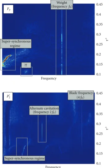
These flow instabilities have been identified from the waterfall plots of Fy, Fz, P"1, and P2", as indicated in Figure5
for N= Nref.
For example, super-synchronous rotating cavitation is clearly detected for 0.15 < τ+ < 0.22. It is identified by the
low frequency that is obtained in the rotating frame from the Fysignal, which is correlated with the peaks that can be
seen from the analysis of P"
2, at frequency fRChigher than the
one of the inducer rotation. This pattern basically consists of large-scale fluctuations of the radial force components Fy
and Fz (Figure6), at frequency that progressively decreases
from a few tens of Hertz down to zero when τ+is decreased.
A 90◦ phase difference between F
y and Fz is observed,
which suggests that these fluctuations may be associated to a rotating instability. Note that the values of the forces are not given in ordinate for confidentiality reasons: only the zero is indicated to facilitate the discussion.
regime Alternate cavitation Blade frequency Weight ?? 0.45 0.4 0.35 0.3 0.25 0.2 0.15 0.1 0.45 0.4 0.35 0.3 0.25 0.2 0.15 0.1 Frequency Frequency (4 f0) P 2 Super-synchronous regime (frequency 2 f0) Super-synchronous Fy (frequency f0) τ + τ +
Figure 5: Waterfall plot for Fyand P"2(Qn, Nref).
Fz
Fy
0
235.2 235.4 235.6 235.8 236 236.2 Time
Figure 6: Time signals of Fyand Fzduring the super-synchronous regime (Qn, Nref, cut-off frequency 400 Hz).
For higher cavitation number (0.22 < τ+ < 0.32), a
stable nonsymmetrical flow pattern is detected. It is mainly characterized by a clear frequency 2 f0 on the spectrum
analysis of P"
1and P2"(see Figure5), which is usually due to
different sheet cavity sizes on successive blades, but identical sheet cavities on opposite blades. Since this arrangement is stable in the rotating frame, no frequency is detected in the waterfall plot of Fyor Fz. Time (s) 120 140 160 180 200 220 240 260 280 300 320 340 50 0 −50 120 140 160 180 200 220 240 260 280 300 320 340 120 140 160 180 200 220 240 260 280 300 320 340 50 0 −50 50 0 −50 120 140 160 180 200 220 240 260 280 300 320 340 50 0 −50 120 140 160 180 200 220 240 260 280 300 320 340 50 0 −50 120 140 160 180 200 220 240 260 280 300 320 340 50 0 −50 120 140 160 180 200 220 240 260 280 300 320 340 50 0 −50 120 140 160 180 200 220 240 260 280 300 320 340 50 0 −50 120 140 160 180 200 220 240 260 280 300 320 340 50 0 −50 120 140 160 180 200 220 240 260 280 300 320 340 50 0 −50 Synchronous regime Super-synchronous regime F=1.3333 Hz F=2.6667 Hz F=5.3333 Hz F=10.6667 Hz F=21.3333 Hz F=42.6667 Hz F=85.3333 Hz F=170.6667 Hz F=341.3333 Hz F=682.6667 Hz
Figure 7: Wavelet decomposition of signal Fy.
In this section we focus on results at speed 1.2 Nref, in
order to have the clearest available fluctuations. Indeed, it has been shown by Coutier-Delgosha et al. (2009) that the rotation speed has some effects on the intensity of the radial loads, but does not modify the instability types.
The decomposition into discrete wavelet (Daubechies n◦5) is applied to the F
ysignal (Figure 7). Frequency f1 is
682 Hz in the present case, and f10 = 1.33 Hz. The analysis
is performed during the pressure decrease between t=120 s and t=340 s, that is from the inception of the first instability regime (alternate cavitation) to the performance breakdown. For high frequencies, high amplitude is nearly systematically obtained, whereas below 100 Hz, several points can be noticed.
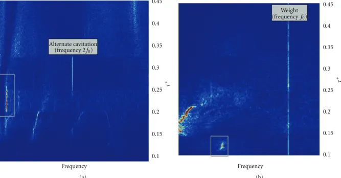
0.45 0.4 0.35 0.3 0.25 0.2 0.15 0.1 τ + Alternate cavitation (frequency 2 f0) Frequency (a) 0.45 0.4 0.35 0.3 0.25 0.2 0.15 0.1 τ + Weight (frequency f0) Frequency (b) Figure 8: Waterfall plot of (a) P"
2and (b) Fy(Qn, 1.2 Nref). 50 0 −50 225 226 227 228 229 230 Time (s) 231 232 233 234 235 Super-synchronous regime
Figure 9: Wavelet decomposition for Fy. Zoom on the time interval 225 s < t < 235 s for f =10.66 Hz (Nref, Qn).
(i) Close to 40 Hz, two sequences are characterized by a significant increase of the intensity: between t=210 s and 230 s (0.19 < τ+ < 0.23), and between t=300 s
and 320 s (0.075 < τ+< 0.09).
(ii) The inception of the super-synchronous instability can be observed clearly in the decomposition at frequency f = 10.66 Hz, and also in the adja-cent decompositions, with a lower intensity. It is observed that this characteristic frequency progres-sively decreases, until a short synchronous regime (which can be detected here at the lowest frequency) is obtained, for 253 s < t < 255 s.
The same process is applied to the unsteady pressure P" 2.
The main resulting information is a very clear unsteadiness characterized by a frequency close to 20/40 Hz for 210 s <
t < 230 s. Such frequency was already observed during the
same time on the Fy signal, but not so clearly. Figure 7
shows the waterfall plot for P"
2at rotation speed 1.2 Nref. A
high-intensity signal at frequency close to 30 Hz is obtained, between the regime of alternate cavitation and the inception of the super-synchronous instability, that is, for 0.19 <
τ+ < 0.23. This corresponds to 210 s < t < 230 s. It can
be noticed that this frequency was much weaker at rotation speed Nref (see Figure 5). Similarly, the second instability
regime detected on the Fy wavelet decomposition (for 300 s < t < 320 s) clearly appears on the waterfall plot at 1.2 Nref,
while it can hardly be detected at speed Nref(cf. Figure5).
It can be concluded that the wavelet decomposition does not enable any better understanding of the mechanisms related to the different instabilities. Conversely, it can be used to detect precisely their inception, as can be seen for example in Figure9in the case of the super-synchronous regime.
5. Analysis of the Temporal Signals
Several types of instabilities are encountered during the process of pressure decrease at 1.2 Nref and Qn. In the
present paper, attention is focused on the regime of alternate cavitation.
This regime is obtained for 130 s < t < 210 s, that is, for 0.23 < τ+ < 0.35. It is characterized by sheet cavities
of different sizes on two consecutive blades but identical on opposite ones. This nonsymmetrical arrangement results in a clear frequency 2 f0on the spectrum analysis of P1"and P"2
(see Figure8). Conversely, no evidence of this unbalanced flow pattern can be found in the waterfall plot of Fy or Fz,
since it is stable in the inducer rotating frame.
Supplementary information can be obtained in the present case from the analysis of the temporal signals: if a low-pass filter with cut-off frequency 100 Hz is applied to the signals of Fyand Fz, in order to get rid of the high-frequency
fluctuations, it becomes clear that mean values of Fyand Fz
are significantly different during all the regime (Figure10). Note that the values of the forces are not given in ordinate for
0
205.7 205.8 205.9 206 206.1 206.2 206.3 206.4 Time
Figure 10: Temporal signals of Fyand Fzwith low pass filter (cut-off frequency 100 Hz), Qn, 1.2 Nref.
1
2
3 4
Figure 11: Plausible configuration for 0.23 < τ+< 0.35. Rectangles
represent schematically the respective lengths of the sheet cavities on the four blades (1.2 Nref, Qn).
confidentiality reasons: only the zero is indicated to facilitate the discussion.
Although the values of the forces are not given in ordinate for confidentiality reasons, it is clear that Fy
fluctuates around a negative average value−Fmean, while Fz
is characterized by a positive mean value close to Fmean. It
implies that the present nonsymmetrical flow pattern causes in addition a constant mean radial force, which does not rotate in the inducer rotating frame. It means that cavitation on opposite blades may not be fully identical. However, the 2 f0 frequency on the pressure waterfall plots shows that
two identical cavitation patterns separated by 180◦ are also
present inside the inducer. The term “cavitation pattern” is voluntary used, since it may concern too sheet cavitation on the blade suction side as tip cavitation close to the inducer shroud.
The most plausible cavitation pattern is thus composed of two identical cavitation areas on two opposite blades (1 and 3), while the two other ones (2 and 4) are both of different size. In this configuration, a constant radial load is obtained in the inducer rotating frame because of the dissymmetry between blades 2 and 4. This load, represented schematically in Figure11, may result (excepted in a particular orientation of axes y and z) in different mean values of the components Fyand Fz.
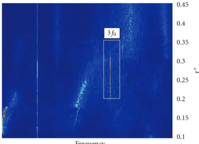
Another feature of the alternate cavitation regime can be remarked on the extended waterfall plots of Fy or Fz (see
Figure 12). Frequency exactly equal to 3 f0 is obtained for
0.23 < τ+< 0.35. 3 f0 0.45 0.4 0.35 0.3 0.25 0.2 0.15 0.1 τ + Frequency
Figure 12: Extended waterfall plot of Fy(Qn, Nref).
Alternate cavitation Breakdown Synchronous regime Frequency 3f0
Figure 13: Extended waterfall plot of Fy(1.18 Qn, Nref).
The following points can be checked from the analysis of the waterfall plots obtained at various rotation speeds and mass flow rates.
(i) It is a 3 f0frequency, which changes with the inducer
rotation speed.
(ii) It can be detected mainly above the nominal flow rate, that is, within the range of mass flow rate that leads to most of the regimes of radial loads. It is particularly strong at high mass flow rate (see Figure13).
(iii) It is not specific to the alternate cavitation flow pattern: all regimes of developed and stable (i.e. nonrotating) cavitation result in the occurrence of the 3 f0 frequency. It is observed for example in the
case presented in Figure13(Nref, 1.18 Qn) that this
frequency is obtained during three successive peri-ods: (1) alternate cavitation, (2) short synchronous regime that occurs just after the super-synchronous one, and (3) regime of highly developed cavitation during the final performance breakdown.
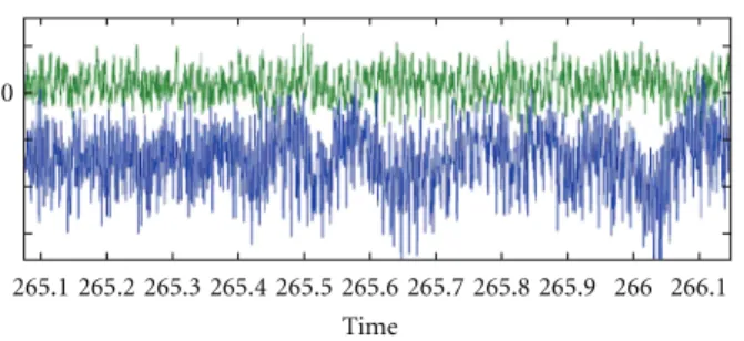
0
265.1 265.2 265.3 265.4 265.5 265.6 265.7 265.8 265.9 266 266.1 Time
Figure 14: Temporal signals of Fy(in blue) and Fz(in green) (Nref,
1.18 Qn).
(iv) The 3 f0 frequency can be detected even in
noncavi-tating conditions, but strongly attenuated.
From these observations, no obvious explanation can be found regarding the occurrence of the 3 f0 frequency.
Con-versely, some points enable to improve the understanding of this phenomenon. For example, no peak at frequency 3 f0is
observed on the waterfall plots of the radial load intensity Fr, whatever the flow configuration is. It means that the radial load does not fluctuate; only its components do. Besides, the 3 f0frequency is clearly detected on the waterfall plots of
the bending moments My and Mz, which suggests that this
instability is related to a shaft bend stress. On the other hand, the frequency peak is very small on the waterfall plots of the axial load Fx, which eliminates any direct connection with an
axial effort on the shaft.
Three different hypotheses can be postulated.
(i) A possible explanation is a rotating perturbation that would rotate at frequency 4 f0in the reference steady
frame, which would generate a frequency 3 f0 in the
inducer rotating frame. Such phenomenon has been observed in experiments conducted in the Osaka University with a three-blade inducer, resulting in a 4 f0 frequency in the inducer frame [10]. It is
called high-order rotating cavitation by Tsujimoto and colleagues. Although the present detected fre-quency is not the same, this example shows that the hypothesis of a perturbation with high rotation speed is plausible. However, it is not the most probable one, because of the exact value 3 f0that is obtained.
(ii) It can be the result of a rotor/stator interaction at the inducer outlet. A method proposed by Brennen [18] enables to obtain the characteristic frequencies related to such interaction. In the present case, the stator in the discharge pipe is equipped with 13 blades, the inducer has 4 blades, so frequencies
f0, 2 f0, 3 f0, and 4 f0 should appear on the plots
with similar intensities. So, frequency 3 f0 should
not be predominant. Still it must be noticed that a frequency range 250 Hz–300 Hz has been previously identified as resonant frequencies of the installation. The 3 f0peak may thus be of higher intensity than the
other ones if it belongs to this range. However this hypothesis is also rejected, because the 3 f0peak is of
high intensity for all rotation speeds, from 0.6 Nrefup
to 1.2 Nref, while the value 3 f0 is not systematically
included into the range of resonant frequencies. (iii) It can be related to a fluctuation of the radial load
angle during the inducer rotation. More precisely, it can be anticipated that several fluctuations occurring during each inducer revolution may result in the measurement of the frequency 3 f0. To investigate
this point, a more in-depth analysis of the temporal signals of Fy and Fz has been conducted during the
alternate cavitation regime for flow conditions Nref
and 1.18 Qn, where frequency 3 f0is remarkably clear
on the waterfall plots. Figure14presents the general aspect of the two signals (Fy in grey Fz in black),
which confirms the difference of mean level that was mentioned previously.
A zoom on a shorter time period is performed in Figure 15(a), to obtain only 25 rotations of the inducer. Oscillations at frequency f0 can be clearly observed on
both signals. Two secondary oscillations of lower amplitude are also detected on the Fy signal, which may explain the
presence of frequency 3 f0 in the spectrum. In the case of Fz, these secondary oscillations do not appear so clearly.
A second zoom is performed to focus on six rotations of the inducer only (see Figure15(b)). Regular oscillations at frequencies f0and 3 f0are observed: the two secondary peaks
are regularly positioned between the main oscillations. On this figure, secondary peaks can be also seen in the signal of component Fz(Figure15(c)). It can be also noticed that the
phase difference between Fyand Fzvaries.
(i) The phase difference at low frequency f0, which
corresponds to the gap between the vertical full lines in Figures 15(b) and 15(c), is small. It equals 90◦,
since it is related to the inducer weight.
(ii) The phase difference between the secondary peaks is not the same. It can be estimated that it is close to 180◦. It means that the phenomenon that generates
the secondary oscillations results in fluctuations of
Fyand Fzcharacterized by phase opposition. It must
be mentioned that the analysis of various periods has enabled to draw this conclusion, while interpretation of Figures15(b)and15(c)is not so clear. On the basis of these observations, no definitive interpretation can be found for frequency 3 f0.
However, a possible explanation, which could be vali-dated only from high-speed visualizations, is given hereafter. It is based on a probable oscillation of the two sheet cavities of different sizes no. 2 and no. 4 denoted in Figure11. These two areas may fluctuate around a mean size, and even reverse (i) because of the vertical pressure gradient due to the gravity within the inducer. The Froude number based on the inducer diameter and the axial velocity is about 0.2, which confirms that the gravity may have some influence on the flow during its passage in the machinery; (ii) or by effect of the two-phase structures which may be different at the top and at the
0 250.15 250.25 250.3 Time 250.2 250.35 250.4 (a) 0 252.22 252.23 252.24 252.25 252.26 252.27 252.28 Time (b) 0 252.22 252.23 252.24 252.25 252.26 252.27 252.28 Time (c)
Figure 15: Zoom on the signals of Fy(in blue) and Fz(in green), 1.18 Qn, Nref, and low pass filter with cut-off frequency 400 Hz.
bottom of the inducer, which would be also an indirect effect of the gravity.
In this case, the oscillation of components Fyand Fz at
frequency f0, due to the inducer weight, may be coupled
to this inversion of sheet cavities 2 and 4, which would occur twice during each rotation of the inducer, leading to a more complex signal. A scheme of the evolutions of Fy
and Fz during a single rotation of the inducer is proposed
in Figure17. It is supposed here that the radial load related to the nonsymmetry between blades 2 and 4 is oriented according to the scheme given in Figure16.
This particular orientation of Fy and Fz enables to
explain the 180◦ phase difference between the two
com-ponents in the secondary oscillations. Indeed, in such configuration, the inversion of the sheet cavities 2 and 4, which makes an inversion of the associated radial load, results in opposite variations of Fyand Fz. It must be noticed
that the blade orientations drawn in Figure 17 represent schematically the direction of the radial load generated by nonidentical sheet cavities on opposite blades. It can be anticipated that these directions are close to the lines that would join the leading edge of the opposite blades.
It is observed in Figure15that the oscillations of Fyare
of larger amplitude than those of Fz, which suggests that the
angle between each component and the blades is not 45◦. As
indicated in Figure16, the direction of Fy may be close to
the direction of the radial load related to the nonsymmetrical flow pattern on blades 2 and 4. The expected evolutions of Fyand Fz during a single inducer rotation are drawn in
Figure17on the basis of this hypothesis.
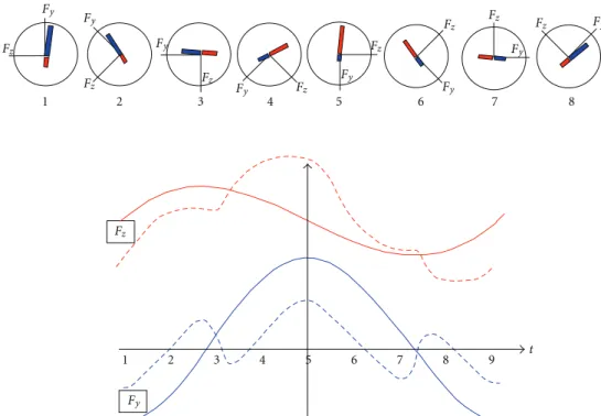
The eight schemes at the top of Figure 16 show the eight successive positions of sheet cavities on blades 2 and 4, during a revolution of the machinery, by step of 45◦. It can
be observed that two inversions of the small and big sheet
1 2 3 4 Fz Fy
Radial load direction
Figure 16: Expected orientation of Fyand Fz, and the blades (1.18 Qn, Nref).
cavities occur during one period, each time they cross the horizontal direction. Between two inversions, the difference of size between sheet cavities 2 and 4 first increases reaching a maximal value, and then decreases. It is maximal when the radial load is vertical, since in such configuration the pressure gradient, which controls the pulsation of the cavities according to our assumption, has the strongest effect on the sheet cavities located on blades 2 and 4.
On the central part of Figure 17, the curves in full line correspond to the evolutions of Fy and Fz without the
radial load generated by the unbalanced flow pattern on blades 2 and 4: a sinusoidal evolution; due to the respective orientations of the gravity, Fy, and Fz, with a π/2 phase
difference between the load components, is obtained in that case. This behaviour is modified by the fluctuations of the sheet cavities on blades 2 and 4, leading to the curves drawn in doted lines.
Fz Fz Fz Fz Fz Fz Fz F z Fz Fy Fy Fy Fy Fy Fy Fy Fy Fy 1 2 3 4 5 6 7 8 1 2 3 4 5 6 7 8 9 t
Figure 17: Scheme of the qualitative evolutions of Fy(blue curve) and Fz(red curve) during a single rotation of the inducer.
The evolution of Fyis composed of the following steps.
(i) It can be anticipated that the radial load will sys-tematically be oriented from the small cavity towards the big one (i.e., from high-pressure areas towards low pressures). So, configuration 1 in Figure 17
is characterized by a component Fy related to the
flow dissymmetry that is positive, and even almost maximal, since blades 2 and 4 are close to the vertical direction. Between steps 1 and 3, the radial load reaches its maximal value, and then it decreases, so the curves in full and dotted lines become closer. It must be reminded that all charts here focus on a qualitative behaviour, while the real evolutions of Fy
and Fzmay depend strongly on the relative values of
the radial load related to the inducer weight and the one related to nonsymmetrical cavitation on blades 2 and 4.
(ii) Just after configuration 3, blades 2 and 4 cross the horizontal direction, so an inversion of the sheet cavity lengths is obtained. Consequently, the radial load due to the dissymmetry, and thus the sign of the
Fycomponent related to this load, is also inverted. It
results in a sudden decrease of Fy, under the curve
in full line. Then, Fy reincreases progressively until
step 5 is reached, since its direction becomes closer to the one of the gravity. In the same time, the radial load due to the dissymmetry also increases, but it is negative, so it slightly counterbalances the effect of the inducer weight.
(iii) Steps 6 to 8 lead to the same variations of Fy, but
in the opposite direction: between steps 5 and 6,
components related to the inducer weight and to the dissymmetry are both decreased. When the leading edges of blades 2 and 4 cross the horizontal direction (just after configuration 7), sheet cavities invert again, so the radial load that they generate also does, and Fy
increases over the full line curve. Then, the effect of the weight decreases, leading to the decrease of Fy.
The curve for Fz is obtained by a similar process: from
steps 1 to 3, the radial load due to sheet cavities on blades 2 and 4 is negative and decreases. After configuration 3, it inverts, so it becomes positive and increases more and more when the sheet cavities get closer to the vertical direction. After configuration 5, the radial load decreases again, and
Fz also does and comes closer to the curve in full line. Just
after step 7, sheet cavities invert again, and the Fzcomponent
related to the dissymmetry becomes negative and decreases down to its value at step 1.
This scenario generates for both components Fy and Fz three successive fluctuations during each rotation of
the inducer, which is consistent with frequency 3 f0 that
is observed on the waterfall plots. In the configuration presented in Figure 17, the three pulsations of Fy occur
at equal distance to each other, which explains the intense peak at frequency 3 f0. Oscillations of component Fz are
not so regular during one rotation, which is consistent with observations from Figure15, and which also explains that the spectral line at 3 f0is weaker for Fzthan for Fy.
6. Conclusion
The instabilities detected in a four-blade inducer have been discussed in the present paper by wavelet decomposition and
analysis of the temporal signals of the two components Fy
and Fzof the radial load on the shaft. It has been found that
wavelet decomposition does not improve the understanding of the flow instabilities, while it enables a precise detection of inception and stop of each unbalanced flow pattern. An unexpected spectral line at 3 f0, which occurs during
alternate cavitation, has been discussed by direct analysis of the temporal signals of Fyand Fz. A possible scenario, based
on the assumption that the gravity may have—directly or indirectly—some effect on the sheet cavities on the blades, is proposed. Only high-speed video would enable to confirm this hypothesis.
Nomenclature
f : Frequency (Hz)
f0: Frequency of the inducer rotation (Hz) Fx: Axial component of the force on the shaft (N) Fy, Fz: Radial components of the force on the shaft (N) N: Rotation speed (s−1)
Nref: Reference rotation speed (s−1)
∆P: Pressure elevation Pd−Pi(Pa) Pi: Absolute pressure in the inlet pipe (Pa) Pd: Absolute pressure in the delivery pipe (Pa) Pti: Total absolute pressure in the inlet pipe (Pa) Ptd: Total absolute pressure in the delivery pipe (Pa) Pvap: Vapor pressure (Pa)
P1", P2": Fluctuating pressures at the inducer inlet (Pa) P3": Fluctuating pressure at the inducer outlet (Pa) Mx: Torque on the inducer shaft (Nm)
My,z: Bending moments on the shaft (Nm) Q: Volume flow rate (m3/s)
Qn: Nominal flow rate (m3/s)
Qm: Main flow rate (in the delivery pipe) (m3/s) Qs: Secondary flow rate (for axial equilibrium) (m3/s) r: Inducer tip radius (m)
t: Time (s)
ν : Outlet ratio hub radius/tip radius (—) Ψ : Head coefficient (Ptd−Pti)/(ρ ω2 r2) (—) χ : Torque coefficient Mx/(ρ ω2r5) (—)
φ : Flow rate coefficient Q/(π ω r3(1−ν2)) (—) τ : Cavitation number (Pti−Pvap)/(ρ ω2r2) (—).
Acknowledgments
The present study was performed in the frame of contractual activity with SNECMA Moteurs and the CNES (French Space Agency). The technical staff of the LML laboratory was much involved in the development and the operation of the test facility. The authors wish to thank especially J. Choquet and P. Olivier for their collaboration.
References
[1] K. Kamijo, T. Shimura, and M. Watanabe, “An experimental investigation of cavitating inducer Instability,” ASME Paper 77-WA/FW-14, 1977.
[2] B. Goirand, A. Mertz, F. Joussellin, and C. Rebattet, “Exper-imental investigation of radial loads induced by partial
cavitation with liquid hydrogen inducer,” in Proceedings of the
3rd International Conference on Cavitation (ImechE ’92), vol.
C453/056, pp. 263–269, Cambridge, UK, 1992.
[3] J. de Bernardi, F. Rossellini, and A. Von Kaenel, “Experimental analysis of instabilities related to cavitation in turbopump inducer,” in Proceedings of the 1st International Symposium on
Pump Noise and Vibrations, pp. 91–99, Paris, France, 1993.
[4] R. A. Furness and S. P. Hutton, “Experimental and theoretical studies of two-dimensional fixed-type cavities,” vol. 97, pp. 515–522, 1975.
[5] Q. Le, J. P. Franc, and J. M. Michel, “Partial cavities: global behavior and mean pressure distribution,” ASME Transactions
Journal of Fluids Engineering, vol. 115, no. 2, pp. 243–248,
1993.
[6] J. B. Leroux, O. Coutier-Delgosha, and J. A. Astolfi, “A joint experimental and numerical study of mechanisms associated to instability of partial cavitation on two-dimensional hydro-foil,” Physics of Fluids, vol. 17, no. 5, article 052101, pp. 1–20, 2005.
[7] O. Coutier-Delgosha, B. Stutz, A. Vabre, and S. Legoupil, “Analysis of cavitating flow structure by experimental and numerical investigations,” Journal of Fluid Mechanics, vol. 578, pp. 171–222, 2007.
[8] Y. Tsujimoto, “Cavitation instabilities in inducers,” Tech. Rep. AVT-143 RTO AVT/VKI Lecture Series, von Karman Institute, Rhode-Saint-Gen`ese, Belgium, 2006.
[9] F. Joussellin, J. De Bernardi, B. Goirand, and Y. Delannoy, “Analyse par films ultrarapides de poches de cavitation sur l’Inducteur de la Turbopompe `a Hydrog`ene d’un Moteur Fus´ee,” in 5`eme colloque de visualisation et de traitement
d’images en M´ecanique des Fluides, Poitiers, France, 1992.
[10] A. Fujii, S. Azuma, Y. Yoshida, Y. Tsujimoto, H. Horiguchi, and S. Watanabe, “Higher order rotating cavitation in an inducer,”
International Journal of Rotating Machinery, vol. 10, no. 4, pp.
241–251, 2004.
[11] O. Coutier-Delgosha, Y. Courtot, F. Joussellin, and J. L. Reboud, “Numerical simulation of the unsteady cavitation behavior of an inducer blade cascade,” AIAA Journal, vol. 42, no. 3, pp. 560–569, 2004.
[12] Y. Yoshida, Y. Sasao, K. Okita, S. Hasegawa, M. Shimagaki, and T. Ikohagi, “Influence of thermodynamic effect on synchronous rotating cavitation,” ASME Transactions Journal
of Fluids Engineering, vol. 129, no. 7, pp. 871–876, 2007.
[13] F. Bakir, S. Kouidri, R. Noguera, and R. Rey, “Experimental analysis of an axial inducer influence of the shape of the blade leading edge on the performances in cavitating regime,” ASME
Transactions Journal of Fluids Engineering, vol. 125, no. 2, pp.
293–301, 2003.
[14] Y. Yoshida, Y. Tsujimoto, D. Kataoka, H. Horiguchi, and F. Wahl, “Effects of alternate leading edge cutback on unsteady cavitation in 4-bladed inducers,” ASME Transactions Journal
of Fluids Engineering, vol. 123, no. 4, pp. 762–770, 2001.
[15] Y. D. Choi, J. Kurokawa, and H. Imamura, “Suppression of cavitation in inducers by J-Grooves,” ASME Transactions
Journal of Fluids Engineering, vol. 129, no. 1, pp. 15–22, 2007.
[16] H. Horiguchi, T. Takashina, and Y. Tsujimoto, “Theoretical analysis of cavitation in inducers with unequally spaced blades,” JSME International Journal, Series B, vol. 49, no. 2, pp. 473–481, 2006.
[17] O. Coutier-Delgosha, G. Caignaert, G. Bois, and J. B. Leroux, “Influence of the blade number on inducer cavitating behav-ior,” Journal of Fluids Engineering. In press.
[18] C. E. Brennen, “Pump vibration, concepts,” in Hydrodynamics