HAL Id: hal-01870216
https://hal.archives-ouvertes.fr/hal-01870216
Submitted on 7 Sep 2018
HAL is a multi-disciplinary open access
archive for the deposit and dissemination of
sci-entific research documents, whether they are
pub-lished or not. The documents may come from
teaching and research institutions in France or
abroad, or from public or private research centers.
L’archive ouverte pluridisciplinaire HAL, est
destinée au dépôt et à la diffusion de documents
scientifiques de niveau recherche, publiés ou non,
émanant des établissements d’enseignement et de
recherche français ou étrangers, des laboratoires
publics ou privés.
Analyzing traces from a Google data center
Pascale Minet, Eric Renault, Ines Khoufi, Selma Boumerdassi
To cite this version:
Pascale Minet, Eric Renault, Ines Khoufi, Selma Boumerdassi. Analyzing traces from a Google data
center. IWCMC 2018 : 14th International Wireless Communications and Mobile Computing
Confer-ence, Jun 2018, Limassol, Cyprus. pp.1167 - 1172, �10.1109/IWCMC.2018.8450304�. �hal-01870216�
Analyzing Traces from a Google Data Center
Pascale Minet
∗Eric Renault
´
†Ines Khoufi
∗and Selma Boumerdassi
‡∗Inria, 2 rue Simone Iff, CS 42112, 75589 Paris Cedex 12, France. Email: [email protected]
† SAMOVAR, Telecom SudParis, CNRS, Universite Paris-Saclay, 91011 Evry, France. Email: [email protected]
‡CNAM/CEDRIC, 292 rue Saint Martin, 75003 Paris, France. Email: [email protected]
Abstract—Traces collected from an operational Google data center over 29 days represent a very rich and useful source of information for understanding the main features of a data center. In this paper, we characterize the strong heterogeneity of jobs and the medium heterogeneity of machine configurations. We analyze the off-periods of machines. We study the distribution of jobs per category, per scheduling class, per priority and per number of tasks. The distribution of job execution durations shows a high disparity, as does the job waiting time before being scheduled. The resource requests in terms of CPU and memory are also analyzed. The distribution of these parameter values is very useful to develop accurate models and algorithms for resource allocation in data centers.
Index Terms—Data analysis, data center, big data application, resource allocation, scheduling.
I. CONTEXT AND MOTIVATION
In High Performance Computing (HPC), it is assumed that all machines are homogeneous in terms of CPU and memory capacities, and that, the tasks making up the jobs have similar resource requests. It has been shown in [1] that this homogeneity relating both to machine capacity and workload , although generally valid for HPC, does no longer apply to data centers. This explains why the publication of data gathered in an operational Google data center over 29 days [2] has aroused such great interest among researchers.
For jobs and tasks, researchers want to characterize their submission, their structure and the workload requested, while for machines, they study the distribution of off-periods. They also highlight any periodic patterns and tendencies, and detect correlations between memory usage and CPU usage if such correlations exist. More generally, they validate or invalidate some simplifying assumptions that are usually made when reasoning about models. Such results are needed to make the models more accurate for jobs and tasks as well as for available machines. Having validated these models on real data centers, they are then used for extensive evaluation of placement and scheduling algorithms and more generally for resource allocation (i.e. CPU and memory). These algorithms can then be applied in real data centers.
Another possible use of this data set is to consider it as a learning set in order to predict some feature of the data center, such as the workload of hosts or the next arrival of jobs. As a conclusion, it is crucial to have real traces of a Google data center publicly available that are representative of the functioning of real data centers. Our goal in this paper is to analyze the data collected and to draw useful conclusions
about machines, jobs and tasks as well as resource usage. In a further step, these results will be integrated in models used in a general framework designed for high performance resource allocation in a data center.
II. RELATED WORK
All the studies so far published relating to this data set [2] include data analysis. In this paper, we also focus on data analysis and draw original conclusions on machine availability, as in [3], [4], jobs and tasks, as in [4], [5], [6] and resource usage, as in [1], [5], [7], [8].
The first lessons drawn from a shorter data set of 6 hours were published in [9]. Although the authors pointed out the presence of peaks in job submissions, the existence of both short jobs and very long ones, the size of this data set is too small to generalize.
Using the 29-day data set published in [2], the authors of [4] show that on average 5.8% of jobs running in a given time window account for 94.7% of CPU usage and 89% of memory usage. They also show that actual resource usage can be approximated by a lognormal distribution. With regard to CPU usage, two thirds of the dominant jobs belonging to normal production exhibit a daily pattern and half of the jobs exhibit a weekly pattern. In addition, the distribution of machine removals shows that the number of removals observed in the trace is higher than that provided by a Poisson distribution, suggesting some spatial or temporal correlations for some machines. However, independent failures with a
failure rate of 10−5 per hour is a reasonable approximation.
A characterization of machines and jobs is provided in [3]. The authors observe that while most machine downtimes are short (i.e less than 25 mn), others may last more than 2 hours and a half. They also show that there are many jobs with a single task, and that most jobs have fewer than 100 tasks, but also that there is a small number of jobs with 2000 tasks. They also point out that on average, a job has 20 scheduling constraints associated with its tasks, which makes such tasks more difficult to place and schedule. An important result is that up to 60% of CPU resource is wasted by tasks that do not complete successfully.
The authors of [5] use K-Means to classify the jobs into three categories according to their duration: short, medium and long. They show that short jobs are the most frequent and use less resources. Medium jobs are frequent and are memory-intensive, i.e. they have strong requirements in
terms of memory. Long jobs, the least frequent, have strong requirements in terms of CPU, and are termed CPU-intensive. The authors of [1] show that 2% of jobs account for 80% of resource usage (i.e. CPU or memory) and that about 75% of jobs run a single task. More generally, they observe that the number of tasks per job is a power of two. The high diversity of resource requests per task is highlighted. The overall memory usage is only 53% of the memory allocation, whereas the CPU usage corresponds to only 40% of the CPU allocation.
In [6], the tasks are classified by means of K-Means and density-based clustering into two categories: CPU-intensive and memory-intensive. The authors propose associating a virtual machine with each task, and their placement algorithm puts two virtual machines of different categories on the same physical machine. However, no performance evaluation is done to validate this approach.
In [8], the authors predict the average load of a host with a Bayesian model. Their method provides a greater accuracy than other methods based on moving averages or auto-regression.
III. DATA PREPROCESSING
A. Real traces
The real traces were collected in an operational Google data center over a period of 29 consecutive days. The goal of the authors of [10] was to point out the complexity of scheduling the jobs submitted to a data center. This complexity is due to the variety of job types, the existence of scheduling constraints for some jobs, the heterogeneity of machines and a bad estimation of resource usage by users.
The confidentiality of these traces is ensured by obfuscation techniques. Each information element recorded has a times-tamp expressed in microseconds. The traces are organized into different tables related to machines, jobs and tasks as well as resource usage. Each table corresponds to several files in the CSV format.
• The M achine events table contains the following
events: add a machine to the data center, remove a machine from the data center, and update the available resources of a machine. It also gives the CPU capacity and the memory capacity of the machine. It has a volume of 2.9 MBytes.
• The M achine attributes table gives the kernel version,
clock speed, etc. of the machine considered.
• The J obs events table and the T ask events table
describe the events related to a job and a task, respec-tively. These events are submit, schedule, evict, fail, finish, kill, update pending and update running. The T asks events table also contains the scheduling class, the priority, the resource request in terms of CPU and memory, as well as some placement constraint of each task. This table has a size of 15.4 GBytes.
• The T asks resource usage includes information about
the mean and maximum usage of memory and CPU
during each measurement period of 5 minutes. It has a size of 159 GBytes.
B. Data cleaning
Before being analyzed, data are cleaned up. Any record with missing information is discarded. The outliers are discarded, for example events occurring at time 0 that were artificially added by the measurement process. To make the processing of records faster, the columns in the different tables that are not analyzed are removed.
IV. MACHINE ANALYSIS
A. Memory and CPU capacities of machines
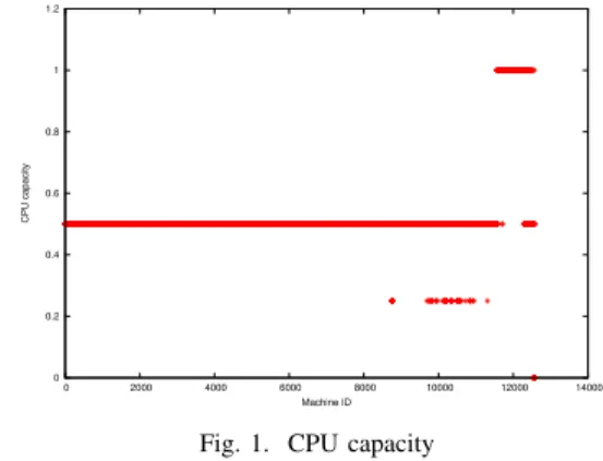
The total number of machines in the data center is 12582. The CPU capacity of any machine is expressed relative to the CPU capacity of the most powerful machine. As a consequence, three types of machines are distinguished, as depicted in Figure 1.
• The most powerful machines with a CPU capacity equal
to 1. There are 796 machines of this type, which corre-sponds to 6.32% of the total number of machines. These machines have consecutive identifiers, which could mean that they have been replaced recently.
• Machines with medium CPU capacity, equal to 0.5. These
represent the largest number of machines (11632) corre-sponding to 92.449% of the total number of machines.
• The least powerful machines with small CPU capacity,
equal to 0.25. There are 123 such machines, which represents 0.977% of the total number of machines. As an initial approximation, machines can be considered as homogeneous in terms of having a CPU capacity equal to 0.5.
0 0.2 0.4 0.6 0.8 1 1.2 0 2000 4000 6000 8000 10000 12000 14000 CPU capacity Machine ID
Fig. 1. CPU capacity
Similarly, the Memory capacity of any machine is ex-pressed relative to the highest Memory capacity. 6 types of machines are distinguished, as depicted in Figure 2.
• Machines with the highest memory capacity have a
Memory capacity in the interval [0.9678, 1]. There are 907 machines of this type, which corresponds to 7.02% of the total number of machines.
• Machines with a Memory capacity of 0.75. These are
1001 such machines, which corresponds to 7.95% of the total number of machines.
• Machines with a Memory capacity in the interval
[0.4995, 0.5]. There are 6712 of these machines, corre-sponding to 53.34% of the total number of machines.
• Machines with a Memory capacity in the interval
[0.2493, 0.25]. There are 3858 machines, which corre-sponds to 30.66% of the total number of machines.
• Machines with a Memory capacity of 0.1241. There are
54 such machines, which corresponds to 0.429% of the total number of machines.
• The least powerful machines with a Memory capacity in
the interval [0.03885, 0.06158]. There are 6 machines of this type, corresponding to 0.047% of the total number of machines.
There is a greater heterogeneity of machines in terms of memory capacity than in CPU capacity. Assuming that the most recent machines have the highest identifiers, we notice that the most recent machines have the highest memory capacity. 0 0.2 0.4 0.6 0.8 1 1.2 0 2000 4000 6000 8000 10000 12000 14000 Memory capacity Machine ID
Fig. 2. Memory capacity.
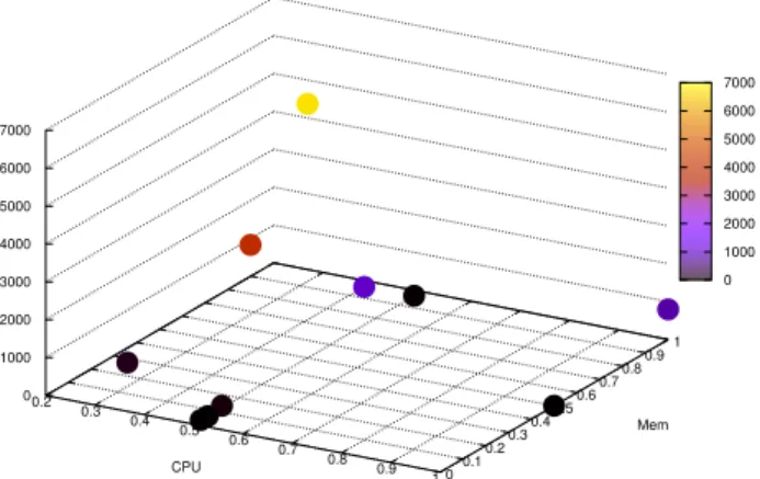
We can now focus on the different machine configura-tions. Each machine configuration is represented by a pair (CP U capacity, memory capacity), as illustrated in Fig-ure 3. We observe the existence of 10 different configurations in the data center. The most frequent configuration, 53% of the machines, corresponds to a CPU capacity ≥ 0.5 and a memory capacity ≥ 0.5. We observe that the machines with the most powerful CPU also have the largest memory capacity. 30% of machines have a CPU capacity of 0.5 and a memory capacity of 0.25. Machine heterogeneity (i.e. 10 different configurations) should be taken into account in the scheduling algorithm. In addition, a uniform distribution model is not appropriate.
Table I shows the percentage of machines per category, given in decreasing order. In a first approximation, we can consider only the first six configurations, the last four config-urations concerning only 0.10% of the machines.
B. Study of machine events
We now focus on the number of changes in machine status. Google defined three types of machine events:
• Add (also called event 0) the machine is added to the set
of operational machines. 0.2 0.3 0.4 0.5 0.6 0.7 0.8 0.9 1 0 0.1 0.2 0.3 0.4 0.5 0.6 0.7 0.8 0.9 1 0 1000 2000 3000 4000 5000 6000 7000 CPU Mem 0 1000 2000 3000 4000 5000 6000 7000
Fig. 3. Number of machines per (CPU, Memory) configuration.
TABLE I
PERCENTAGE OF MACHINES PER CONFIGURATION.
CPU capacity Memory capacity Percentage of machines
0.5 0.5 53.45% 0.5 0.25 30.73% 0.5 0.75 7.97% 1 1 6.31% 0.25 0.25 0.98% 0.5 0.125 0.43% 0.5 0.03 0.039% 0.5 1 0.031% 1 0.5 0.023% 0.5 0.06 0.007%
• Remove (also called event 1) the machine is no longer
operational. It has either failed or is undergoing mainte-nance.
• Update (also called event 2) the resources (e.g. CPU or
memory or system version) of the machine are updated. Figure 4 depicts the number of machines on a logarithmic scale having a given number of adds, removes and updates per machine. The number of machines having had a given number of removes is equal to the number of machines having had the same number of adds. This seems to indicate that each machine that has been removed has finally been added. The number of updates is higher than the number of adds and removes. We observe that very few machines, 4, have a number of changes higher that 50, which corresponds to 0.03%. A very large number of machines, 12540, corresponding to 99.66% of all the machines have a number of changes less than or equal to 10. The three curves (i.e. add, remove and update) follow a hyperbolic pattern.
There were 8860 remove events followed by an add event, corresponding to machine restarts. The duration of these off-periods is depicted in Figure 5. It varies from 5 seconds to 1044365 seconds, corresponding to 11.5 days. 1 machine was unavailable for 11.5 days. 50% of off-periods were less than or equal to 1000 seconds. 1% of the off-periods has a duration equal to 1000 seconds. The number of off-periods equal to a given duration higher than 1000 seconds is equal to 1 or 2.
1 10 100 1000 10000 0 20 40 60 80 100 120 140 160 180 Number of machines
Number of event’s changes
Event 0 Event 1 Event 2
Fig. 4. Number of adds(0), removes(1) and updates(2) per machine.
20 40 60 80 100 120 900 1000 1100 Number of periods
Duration of Off-On periods
Distribution of Off-On periods 20 40 60 80 100 120 1 10 100 1000 10000 100000 1e+06 Number of periods
Duration of Off-On periods
Distribution of Off-On periods
Fig. 5. Number of off-periods with a given duration.
V. PATTERN OF JOB SUBMISSIONS
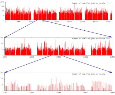
We compute the number of jobs submitted per minute. observing the distribution of job submissions over the 29 days a repetitive and fractal pattern becomes apparent, as depicted in Figure 6. We observe a periodicity of 10, 100, 1000 and 10000. This means that every 10 minutes we observe an absence of submissions for 1 minute; every 100 minutes an absence of job submissions for 10 minutes; every 1000 minutes an absence of job submissions for 100 minutes; every 10000 minutes an absence of job submissions during 1000 minutes. An absence of job submissions does not mean that no job arrives in the data center but that no job is released by the global scheduler. This regularity cannot be explained by randomness. It should correspond to some periodic management task run in the Google data center.
Fig. 6. Repetitive pattern in the job submission.
VI. ANALYSIS OF JOBS AND TASKS
From the T ask Event table, we compute the following three distributions: the priority of jobs, the scheduling class of jobs and the number of tasks per job.
The priority of jobs ranges from 0 to 11. Depending on its priority, a job belongs to one of the following five categories defined in [1]:
• F ree with the lowest priorities 0 and 1. Such jobs incur
little charging.
• P roduction with priority 9.
• M onitoring with priority 10. These jobs are in charge
of monitoring the health of other jobs.
• Inf rastructure with the highest priority 11. These jobs
deal with the infrastructure of the data center.
• Other with priorities 2 to 8.
Table II provides the distribution of jobs in the different categories.
TABLE II
PERCENTAGE OF JOBS PER CATEGORY.
Category Priorities Percentage of jobs
Free 0 or 1 33.63%
Other 2 to 8 56.30%
Production 9 9.91%
Monitoring 10 0.13%
Infrastructure 11 0.002%
Figure 7 depicts the number of jobs per priority on a logarithmic scale. There is no job in priority 7. As expected, there is only 1 job having the highest priority 11 which is reserved to the infrastructure. The number of jobs with a priority equal to 3 or 5 is equal to 100, for both. The numbers of jobs having a priority of 0, 1, 4, 6, 8 or 9 is close to 100000. Here again, a uniform distribution of jobs in the different priorities does not apply.
0.1 1 10 100 1000 10000 100000 1e+06 0 2 4 6 8 10 Number of jobs Priority
Distribution of jobs per priority
Fig. 7. Number of jobs per priority.
The scheduling class of a job indicates the latency sensitiv-ity of this job, where 0 denotes a non-production task and 3 a latency-sensitive task. Figure 8 depicts the number of jobs per scheduling class. As expected, there is a very small number of jobs, 2364, that are latency-sensitive, with a scheduling class equal to 3. Most jobs, 178959, belong to the scheduling class 1, whereas remaining jobs are more or less evenly distributed in the scheduling classes 0 and 2, with about 12000. Table III provides the percentage of jobs per scheduling class.
0 50000 100000 150000 200000 0 1 2 3 Number of jobs Scheduling class
Distribution of jobs per scheduling class
Fig. 8. Number of jobs per scheduling class. TABLE III
PERCENTAGE OF JOBS PER SCHEDULING CLASS.
Scheduling class Percentage of jobs
0 30.3%
1 42.65%
2 26.45%
3 0.5%
The number of tasks per job is depicted in Figure 9 on a logarithmic scale on both axes. 92.05% of jobs have a single task. 95.75% of jobs have fewer than 10 tasks, 98.6% of jobs have fewer than 50 tasks and 99% of tasks have fewer than 92 tasks. We also notice that 1 job has a number of tasks equal to 10500 and 12 jobs have a number of tasks equal to 5000. The number of tasks per job is frequently a multiple of 10.
VII. RESOURCE REQUESTS ANDJOB EXECUTION
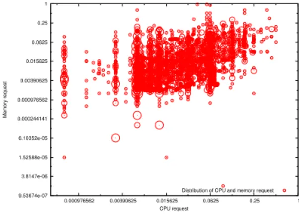
From the Task Event table, we compute the distribution of CPU requests and memory requests per job shown in Figure 10. We observe that all the tasks of a same job request the same amount of CPU and the same amount of memory. We notice that: 1 10 100 1000 10000 100000 1 10 100 1000 10000 Number of jobs Number of tasks
Distribution of tasks per job
Fig. 9. Distribution of the number of tasks per job.
• 1.54% of jobs have a CPU request higher than or equal
to 10%
• 1.74% of jobs have a memory request higher than or
equal to 10%.
• 0.11% of jobs have a memory request and a CPU request
higher than or equal to 10%.
In Figure 10, where the x-axis and the y-axis are represented with a log base 2 scale, many CPU and memory requests are ”aligned”. This means that some specific values are preferred over others. An in-depth analysis shows that most of the ”lines” are powers of 2. In other words, memory requests and CPU requests are often expressed as powers of 2.
9.53674e-07 3.8147e-06 1.52588e-05 6.10352e-05 0.000244141 0.000976562 0.00390625 0.015625 0.0625 0.25 1 0.000976562 0.00390625 0.015625 0.0625 0.25 1 Memory request CPU request
Distribution of CPU and memory request
Fig. 10. Distribution of CPU and memory requests.
We first focus on the time jobs must wait before being scheduled. This time is called job schedule time. The distribu-tion of job schedule times is depicted in Figure 11. 60% of jobs wait 1 second before being scheduled. 94.25% of jobs wait less than 10 seconds. Surprisingly, there are 50 jobs (0.013%) that wait more than 1000 seconds. One possible explanation could be that they request specific resources that are not immediately available.
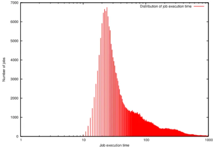
The job execution time is evaluated from the schedule time up to the completion time of the last task. The distribution of the job execution times is illustrated in Figure 12. 35122 jobs do not finish within the 29-day period. considered in the dataset. 384362 jobs finish successfully, corresponding to
1 10 100 1000 10000 100000 1e+06 1 10 100 1000 10000 100000 1e+06 Number of jobs
Job schedule time
Distribution of job schedule time
Fig. 11. Distribution of job schedule times.
91.62% of all the jobs. 4 jobs have an execution time less than 10 seconds. About 36000 jobs, representing 9% of the jobs have an execution time within the interval [20, 25] seconds. Most jobs, 49%, have an execution less less than 100 seconds. 90% of jobs have a duration less than 1000 seconds. We observe that the number of jobs with an execution time equal to 1000×n, with n a positive integer, is approximately divided by two, each time n is increased by 1.
0 1000 2000 3000 4000 5000 6000 7000 1 10 100 1000 Number of jobs
Job execution time
Distribution of job execution time
Fig. 12. Distribution of job execution times.
VIII. CONCLUSION
The data set obtained from an operational data center over 29 days provides very interesting information. Data analysis allows us to draw the following conclusions.
• Although 92.45% of machines have a CPU capacity of
0.5, there are 10 machine configurations in the data center, each configuration is characterized by a pair (CP U capacity, memory capacity). The most frequent configuration is supported by only 53.34% of machines.
• Over the 29 days, all the machines in the data center
that were removed, were restarted later after an off-period. 50% of these periods have a duration less than or equal to 1000 seconds (i.e. 16.66 minutes), suggesting a maintenance operation.
• The study of the number of job submissions per minute
shows an unexpected fractal pattern with a periodicity of 10, 100, 1000 and 10000 minutes, where every 10 minutes there is an absence of submissions for 1 minute, and so on. This could be explained by the fact that the global scheduler could be periodically unavailable to allow some management of the data center infrastructure to take place.
• The distribution of jobs per category reveals only one
job, representing 0.002%, for the Infrastructure, 0.13% of jobs for Monitoring, 9.91% of jobs for Production, 56.30% of jobs for Other, and 33.63% of jobs for Free. 92.05% of jobs have a single task. 95.75% have fewer than 10 tasks. But 12 jobs have 5000 tasks and 114 jobs have around 1000 tasks.
• With regard to resource requests, 0.11% of jobs have a
memory request and a CPU request higher than or equal to 10%.
• 94.25% of jobs wait less than 10 seconds before being
scheduled. However, some of them wait for more than 1000 seconds. Such large values could be explained by the existence of placement constraints for the jobs, making them harder to place and schedule. 49% of jobs have an execution time less than 100 seconds.
These features should be reflected in the job sets and the models used to evaluate the performances of scheduling place-ment algorithms in data centers.
REFERENCES
[1] C. Reiss, A. Tumanov, G. R. Ganger, R. H. Katz, and M. A. Kozuch, “Heterogeneity and dynamicity of clouds at scale: Google trace analy-sis,” in ACM Symposium on Cloud Computing (SoCC), San Jose, CA, USA, Oct. 2012.
[2] J. Wilkes, “More Google cluster data,” Google research blog, Nov. 2011. [3] Z. Liu and S. Cho, “Characterizing machines and workloads on a Google cluster,” in 8th International Workshop on Scheduling and Resource Management for Parallel and Distributed Systems (SRMPDS), Pittsburgh, PA, USA, Sep. 2012.
[4] O. Beaumont, L. Eyraud-Dubois, and J.-A. Lorenzo-Del-Castillo, “An-alyzing real cluster data for formulating allocation algorithms in Cloud platforms,” in 2-th International Symposium on Computer architecture and High Performance Computing (SBAC-PAD), Paris, France, Oct. 2014.
[5] M. Alam, K. A. Shakil, and S. Sethi, “Analysis and clustering of workload in google cluster trace based on resource usage,” CoRR, vol. abs/1501.01426, 2015.
[6] S. Yousif and A. Al-Dulaimy, “Clustering cloud workload traces to improve the performance of cloud data centers,” in Proceedings of the World Congress on Engineering 2017, (WCE2017), 07 2017. [7] . R. F. Gbaguidi, S. Boumerdassi and E. Ezin, “Characterizing servers
workload in Cloud Datacenters,” in International Conference on Future Internet of Things and Cloud (FiCloud 2015), Roma, Italy, August 2015, pp. 20–25.
[8] S. Di, D. Kondo, and W. Cirne, “Host load prediction in a google com-pute cloud with a bayesian model,” in Proceedings of the International Conference on High Performance Computing, Networking, Storage and Analysis, ser. SC ’12, 2012, pp. 21:1–21:11.
[9] Y. Chen, A. S. Ganapathi, R. Griffith, and R. H. Katz, “Analysis and lessons from a publicly available google cluster trace,” EECS Department, University of California, Berkeley, Tech. Rep., Jun 2010. [10] C. Reiss, J. Wilkes, and J. L. Hellerstein, “Google cluster-usage traces:
format + schema,” Google Inc., Mountain View, CA, USA, Technical Report, Nov. 2011.