Spatio-temporal convolutional neural networks for failure prediction

HAL Id: hal-02282219

https://hal.archives-ouvertes.fr/hal-02282219

Submitted on 9 Sep 2019

HAL is a multi-disciplinary open access

archive for the deposit and dissemination of

sci-entific research documents, whether they are

pub-lished or not. The documents may come from

teaching and research institutions in France or

abroad, or from public or private research centers.

L’archive ouverte pluridisciplinaire HAL, est

destinée au dépôt et à la diffusion de documents

scientifiques de niveau recherche, publiés ou non,

émanant des établissements d’enseignement et de

recherche français ou étrangers, des laboratoires

publics ou privés.

Spatio-temporal convolutional neural networks for

failure prediction

Nicolas Aussel, Fabian Dubourvieux, Yohan Petetin

To cite this version:

Nicolas Aussel, Fabian Dubourvieux, Yohan Petetin. Spatio-temporal convolutional neural networks

for failure prediction. GRETSI 2019: XXVIIème colloque francophone de traitement du signal et des

images, Aug 2019, Lille, France. pp.1-5. �hal-02282219�

Spatio-temporal convolutional neural networks for failure

prediction

Nicolas Aussel1,2, Fabian Dubourvieux1,2, Yohan Petetin2,

1_{TriaGnoSys GmbH}

Argelsrieder Feld 22, 82234 Wessling, Germany

2_{Télécom SudParis / Département CITI et CNRS UMR 5157}

9 Rue Charles Fourier, 91011 Evry, France

nicolas.aussel@telecom-sudparis.eu, fabian.dubourvieux@telecom-sudparis.eu yohan.petetin@telecom-sudparis.eu

Résumé – L’utilisation de techniques d’apprentissage statistique pour identifier une panne au sein d’un système à partir de séries temporelles intrinsèques à ce système est bien connu. Néanmoins, dans le cadre d’un système industriel composé de plusieurs sous systèmes, l’application directe de ces techniques au système global est limitée par la complexité de celui-ci, tandis que leur application sur chacun des sous systèmes ne prend pas en compte les dépendances qui peuvent intervenir entre eux et mènent à des performances faibles. L’objectif de cette communication est de proposer un modèle de réseau de neurones convolutionnels spatio-temporels capable de prendre en compte à la fois des dépendances spatiales et temporelles de séries temporelles observées par des sous systèmes pour la classification de pannes dans un système industriel.

Abstract – The use of statistical learning techniques to identify a failure in a system by using time series collected from it is well known. However, in the case of an industrial system made of multiple subsystems, their direct application is limited by the system complexity. In the meantime, the application of those techniques individually to each subsystem does not take their dependencies into consideration leading to limited performances. The objective of this paper is to propose a model of spatio-temporal convolutional neural network able to consider spatial and spatio-temporal dependencies on time series collected on subsystems of an industrial system for failure classification.

1

Introduction

1.1

Failure prediction of an industrial

sys-tem

There are multiple challenges specific to failure predic-tion of complex industrial systems to keep in mind when designing a statistical method to identify and prevent fai-lures.

First, the occurrence of a failure in an industrial system is (hopefully) quite rare. This is obviously desirable from a user’s perspective but it is a source of difficulties for failure classification as many learning techniques for classification operate best when the proportion between the two classes to learn is close to 1 [1]. Rare event classification with im-balance ratio such 1 to 10.000 is a constraint that need to be taken into account when designing a failure prediction algorithm.

The second difficulty that can arise when working on a complex industrial system is precisely its complex nature. There are several ways for this complexity to create issues but for this contribution we will focus on two specific ones. The first one is that it might not make sense to try to

mo-del the behaviour of a complex system as a single entity. A more efficient approach would be to model individual subsystems and their interactions but these interactions can introduce dependencies that need to be accounted for. In our application case, the subsystems considered are all part of the same network with a ring topology that intro-duces spatial dependencies. Indeed, as neighbouring sub-systems from a network perspective can affect each other, it is no longer sufficient to apply a learning method indi-vidually to each subsystem. The second issue we consider is that for a complex system, the information collected at each time step is not necessarily sufficient to fully describe its state. It can be necessary to consider the information with regards to the previously known state of the system which in other words means that time dependencies are present.

Classical learning methods that can deal with those constraints exist. In the case of time dependencies, tech-niques related to time series analysis are adapted and, in the case of spatial dependencies, techniques related deep learning and in particular to convolutional neural net-works are often the most efficient. However, when

consi-dering both constraints at once, the solutions are more limited. To that end, we consider a variant of convolutio-nal neural network called spatio-temporal convolutioconvolutio-nal neural network initially developed for video classification and show how it can be transposed to failure classification of an industrial system.

In this paper, we will first give a brief overview of the currently widespread model of convolutional neural net-work. Then we detail the variant that we will consider of spatio-temporal convolutional neural network. Then we present the modifications we made to adapt it to the fai-lure classification problem.

1.2

Neural networks

1.2.1 Deep Neural Networks

Fully connected Deep Neural Networks (DNN) are po-pular architectures which aim at approximating a com-plex unknown function f (x), where x ∈ Rn _{is an}

observa-tion, by fθ(x) [2] [3]. θ consists of the parameters of the

DNN, the bias vectors b(i)_{and the weight matrices W}(i)

for all i, 1 ≤ i ≤ P where P is the number of layers of the DNN, and fθ(x) is a sequential composition of linear

functions built from the bias and from the weights, and of a non-linear activation function g(.) (eg. the sigmoid g(z) = 1/(1 + exp(−z)) or the rectified linear unit (ReLu) g(z) = max(0, z)) [4][5].

Parameters θ = {b(i)_{, W}(i)_{} are estimated from the}

back-propagation algorithm via a gradient descent method based on the minimization of a cost function Lθ((x1, y1),

· · · , (xN, yN)) deduced from a training dataset [6].

However, when the objective is to classify high dimen-sional data such as colour images with a large number of pixels, fully connected DNN are no longer adapted from a computational point of view.

1.2.2 Convolutional neural networks

Convolutional Neural Networks (CNN) aim at dealing with the previous issue by taking into account the spatial dependencies of the data [7]. More precisely, data are now represented by a 3-D matrix where the two first dimen-sions represent the height and the width of the image while the depth represents the three colour channels (R,G,B).

Next, as fully connected DNN, CNN consists in buil-ding a function fθ(x), where x ∈ Rd1× Rd2× Rd3, by the

sequential composition of the following elementary steps : • a convolution step via the application of convolution filters on the current image. Each filter is described by a matrix with appropriate dimensions ;

• the application of an activation function g(.) such as the ReLu ;

• a pooling step to reduce the dimension of the resul-ting image.

After the recursive application of these three steps, the

Figure 1 – Example of a CNN architecture output image is transformed into a vector of Rn _{and is}

classified via a fully DNN described in the previous para-graph [8]. A general CNN architecture is displayed in Fig. 1.2.2.

Again, the back-propagation algorithm estimates the parameters (weights and bias of the final DNN and of the convolution matrices) of the CNN.

2

Architectural design

Our system consists of a collection of subsystems or-ganized in a ring network. Each subsystem produces log messages describing events relative to its operational sta-tus. We first propose a log parsing technique to transform these logs then we propose an architecture based on CNN to predict failures.

2.1

Features

The information collected for our use case is in the form of log messages in full text, similar to syslog messages of linux systems and collected by each subsystem. As text is not a suitable input for the spatio-temporal convolutional neural network, we parse those messages using the Na-tural Language Processing approach described in [9]. To summarize this process, the logs follows four main steps : First, the messages are broken down in individual words through a standard tokenizer. The words are then regrou-ped in tuples using a n-gram approach. Following this, a hashing trick is used to compress the model in order to minimize its memory footprint. Finally, a Latent Dirichlet Allocation (LDA) is applied to clusterize the messages by topic and the original log messages are mapped into their vector of topic distribution.

As the industrial system studied here is the same that this method was first developed on, we simply keep the same parameters that were found optimal in [9], namely, we use a bi-gram approach and a number of topic for the LDA of 50.

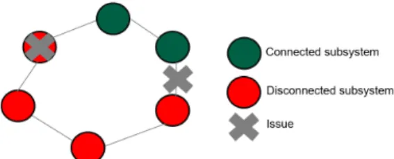
Each subsystem generates logs and the system itself is a ring network of the subsystems. The failures that we aim to classify are loss of connectivity of the subsystems. The figure 2.1 shows an example of failure in a simplified network.

Figure 2 – Example of subsystem failures in a simplified network

2.2

Spatio-temporal convolutional neural

network

We now consider a variant of the general CNN presen-ted in Paragraph 1.2 which is based on spatio-temporal CNN developed to classify data video streaming [10] [11]. Such architectures are indeed adapted to multiple subsys-tems connected in a ring network when the objective is to estimate the failure probability of each subsystem in the future by taking into account i) the spatial dependencies of the global system and ii) the temporal dependencies of the observed data.

More precisely, we set dtime as the size of the time

window, Nf as the number of observed features of each

subsystem during dtime and Ns as the number of

subsys-tems which compose the global system. At time t, the global system is described by a 3D matrix x = (xt,j,k),

1 ≤ t ≤ dtime, 1 ≤ j ≤ Ns, 1 ≤ k ≤ Nf, where the term

xt,j,k coincides with the value of the k-th feature at time

t, for the j-th subsystem. We conserve spatial topology of the problem by ensuring that the subsystems of features

x.,j−1,.and x.,j+1,.are the 2 neighbours in the ring graph

of the system of features x.,j,..

In the intermediate layers, the architecture relies on 2D convolution filters, that is to say that the filters are des-cribed by a 3D matrix with the same depth as the original input, contrary to 3D convolution filters. The reason why is that we want to emphasize on the dependency between the temporal and the spatial dimensions for a given feature and not on that of the different features between them-selves. It is why that contrary to spatio-temporal CNN developed for video streaming, the temporal dimension coincides now with the first dimension of the input.

Next, our architecture is based on deep residual lear-ning. Roughly speaking, a bloc of convolution and poo-ling layers in the classical CNN presented in paragraph 1.2.2 learns directly an intermediate function H(x). Resi-dual learning consists in learning an intermediate resiResi-dual function F (x) = H(x) − x rather than H(x) directly. In-tuitively, this approach reduces the difficulty when a bloc of convolution and pooling layers aims at approximating an identity mapping, in particular in CNN with a large number of layers [12].

Finally, for a given subsystem the global architecture approximates the probability of a failure at time t + 1

given the past observations from time t − dtime+ 1 until

t, x, i.e. it computes Pθ(y(j)= 1|x) for all j, 1 ≤ j ≤ Ns.

2.3

Detail of the architectures and

imple-mentation

2.3.1 Loss function

Let ((x1, y1), · · · , (xN, yN)) be our training set, with xi

being the input processed as described in 2.2 for a certain range of time and yi = (y

(1)

i , ..., y

(Ns)

i ) the sequence of

binary labels of the subsystems at the next time step. The function fθ(x) = (f

(1)

θ (x), · · · , f

(Ns)

θ (x)) computed by our

CNN aims at estimating the probabilities of failure of the subsystems given a new input x.

To that end, we assume that the probabilities of failure of the subsystems are independent given x (the conditional independence is a modelling choice motivated by compu-tation limits and does not mean that the marginals y_ijare independent for a fixed i),

Pθ(yi|xi) = Pθ(y (1) i |xi) × · · · × Pθ(y (Ns) i |xi), with Pθ(y (j) i |xi) = f (j) θ (xi)y (j) i × (1 − f(j) θ (xi))(1−y (j) i ).

The minimum negative log-likelihood estimate of θ is given by argminθLθ(x, y) where

Lθ(x, y) = N X i=1 Ns X j=1 L(j)_θ (xi, yi)

and where L(j)_θ (xi, yi) = −y

(j) i ×log(f (j) θ (xi))−(1−y (j) i )×

log(1 − f_θ(j)(xi)) is the binary classification loss for the

subsystem j.

2.3.2 Architecture details

The architecture of our neural network is the ResNet181. It is a 18 layer CNN with a fully-connected last layer where we apply the sigmoid function to enforce fθ(x) to belong

to [0, 1]Ns_{, with the result being interpreted as the}

proba-bility for a failure to occur for each subsystem. The size of filters are modified to fit our spatio-temporal model as in 2.2. We manage the problem of rare events by balancing the training mini batch of data. We use a batch size of 32 and a learning rate of 0.01 to minimize Lθ(x, y). Finally,

we use a time window of size 100 selected to maintain a manageable memory footprint for our method.

We implemented this model with PyTorch2 _running

over CUDA3 _{except for the log parsing step described}

before which is implemented on Spark4 with a Python interface.

1. https ://github.com/pytorch/vision/blob/master/torchvision/models/resnet.py 2. https ://pytorch.org/

3. https ://developer.nvidia.com/cuda-zone 4. https ://spark.apache.org/

3

Simulation

3.1

Metrics

For performance evaluation, we report precision and re-call. By considering the failure of a subsystem as a posi-tive, they are given by :

P recision = T rueP ositives

T rueP ositives + F alseP ositives

Recall = T rueP ositives

T rueP ositives + F alseN egatives Those metrics are selected instead of the more standard accuracy for their robustness to class imbalance. Indeed, in the situation considered, negative samples outnumber positive samples by a factor 10, 000 meaning that a naive classifier always outputting negative predictions regardless of its input would reach 99.99% accuracy.

We also use 3-fold stratified cross-validation in order to ensure that the measurement are reliable, given the rela-tively low number of positive samples in the dataset. The stratification is done to ensure that a similar number of positive sample remains in every split as small variations could potentially results in large variations of the class imbalance ratio in the splits.

3.2

Results and conclusion

The performances reached by our architecture are 11.3% precision and 3.42% recall. These results are very encoura-ging compared to the decision tree-based approaches tes-ted before on the same use case. On this dataset, more traditional learning methods such as Random Forest and Gradient Boosted Trees provide no results at all with 0% precision and recall. The spatio-temporal convolutional neural network that we describe is the first method to provide non zero results.

Our interpretation is that even though the traditional methods proved useful in studying other kind of failures of this system in [9] they are only able to model time depen-dencies which are not sufficient here. This highlight the importance for industrial applications of developing mo-dels that can take into account dependencies that match the systems actually in place.

It is important to note however that, while this result is encouraging, because of constraints on computation re-sources such as memory and computation power, a full architectural search is still in progress in order to deter-mine the exact parameters of the neural network that can optimize the performances.

Références

[1] N. Japkowicz and S. Stephen, “The class imbalance problem : A systematic study,” Intelligent data ana-lysis, vol. 6, no. 5, pp. 429–449, 2002.

[2] F. Rosenblatt, “The perceptron–a perceiving and re-cognizing automaton,” Tech. Rep. 85-460-1, Cornell Aeronautical Laboratory, 1957.

[3] M. Negnevitsky, Artificial Intelligence : A Guide to Intelligent Systems. Boston, MA, USA : Addison-Wesley Longman Publishing Co., Inc., 1st ed., 2001. [4] G. Cybenko, “Approximation by superpositions of a sigmoidal function,” Mathematics of Control, Signals, and Systems (MCSS), vol. 2, pp. 303–314, Dec. 1989. [5] Y. LeCun, Y. Bengio, and G. E. Hinton, “Deep lear-ning,” Nature, vol. 521, no. 7553, pp. 436–444, 2015. [6] D. E. Rumelhart, G. E. Hinton, and R. J. Williams, “Neurocomputing : Foundations of re-search,” ch. Learning Representations by Back-propagating Errors, pp. 696–699, Cambridge, MA, USA : MIT Press, 1988.

[7] S. Albawi, T. A. Mohammed, and S. Al-Zawi, “Un-derstanding of a convolutional neural network,” in 2017 International Conference on Engineering and Technology (ICET), pp. 1–6, Aug 2017.

[8] A. Krizhevsky, I. Sutskever, and G. E. Hinton, “Ima-genet classification with deep convolutional neural networks,” in Proceedings of the 25th International Conference on Neural Information Processing Sys-tems - Volume 1, NIPS’12, (USA), pp. 1097–1105, Curran Associates Inc., 2012.

[9] N. Aussel, Y. Petetin, and S. Chabridon, “Improving performances of log mining for anomaly prediction through nlp-based log parsing,” 2018 IEEE 26th In-ternational Symposium on Modeling, Analysis, and Simulation of Computer and Telecommunication Sys-tems (MASCOTS), pp. 237–243, 2018.

[10] K. Simonyan and A. Zisserman, “Two-stream convo-lutional networks for action recognition in videos,” in Proceedings of the 27th International Conference on Neural Information Processing Systems - Volume 1, NIPS’14, (Cambridge, MA, USA), pp. 568–576, MIT Press, 2014.

[11] D. Tran, L. Bourdev, R. Fergus, L. Torresani, and M. Paluri, “Learning spatiotemporal features with 3d convolutional networks,” in Proceedings of the 2015 IEEE International Conference on Computer Vision (ICCV), ICCV ’15, (Washington, DC, USA), pp. 4489–4497, IEEE Computer Society, 2015. [12] K. He, X. Zhang, S. Ren, and J. Sun, “Deep residual

learning for image recognition,” in 2016 IEEE Confe-rence on Computer Vision and Pattern Recognition, CVPR 2016, Las Vegas, NV, USA, June 27-30, 2016, pp. 770–778, 2016.