HAL Id: hal-01718082
https://hal.archives-ouvertes.fr/hal-01718082
Submitted on 1 Jun 2018
HAL is a multi-disciplinary open access
archive for the deposit and dissemination of sci-entific research documents, whether they are pub-lished or not. The documents may come from teaching and research institutions in France or abroad, or from public or private research centers.
L’archive ouverte pluridisciplinaire HAL, est destinée au dépôt et à la diffusion de documents scientifiques de niveau recherche, publiés ou non, émanant des établissements d’enseignement et de recherche français ou étrangers, des laboratoires publics ou privés.
Determination of reaction parameters for cardboard
thermal degradation using experimental data
T Loulou, Sylvain Salvador, Jean-Louis Dirion
To cite this version:
T Loulou, Sylvain Salvador, Jean-Louis Dirion. Determination of reaction parameters for cardboard thermal degradation using experimental data. Chemical Engineering Research and Design, Elsevier, 2003, 81 (A9), pp.1265-1270. �10.1205/026387603770866489�. �hal-01718082�
DETERMINATION OF REACTION PARAMETERS FOR
CARDBOARD THERMAL DEGRADATION USING
EXPERIMENTAL DATA
T. LOULOU, S. SALVADOR and J. L. DIRION
Ecole des Mines d’Albi-Carmaux, Laboratoire de Gnie des Procds des solides diviss, UMR CNRS 2393 Albi, France
T
his work is part of an ongoing research effort in which parameter estimation techniques have been utilized in recovering the kinetic parameters of a given reacting model using measurements collected from TGA devices. The goal of this research work is to develop a useful and universal estimation procedure to determine simultaneously the kinetic parameters involved in the chemical modelling under study such as combustion, pyrolysis, waste stabilization, etc. The present parameter estimation problem is solved with the Levenberg–Marquardt method of minimization of the least square norm representing the square difference between the measured mass variations during cardboard pyrolysis and the mass responses obtained with numerical solution of the model. An analysis of the linear dependency of the pyrolysis parameters needed to design a robust estimation tool is presented. In order to perform this analysis, the sensitivity coefécients and the sensitivity matrix determinant were examined. Experimental data obtained with TGA during the pyrolysis process of cardboard are analysed in this paper and the unknown parameters involved in the kinetic modelling are estimated.Keywords: parameter estimation; inverse problem; sensitivity coefécient; kinetic model.
INTRODUCTION
In building the reaction schemes for solids decomposition, the estimation of kinetic parameters represents a crucial step in chemical modelling (Font et al., 2001). Indeed, once a kinetic scheme has been established, two main methods can be used to estimate the corresponding Arrhenius parameters: a graphical method and numerical étting. The érst method is usually limited to a global (single) reaction. When the reacting scheme involves more than one reaction, the graphic method is not adequate and the numerical étting represents the only alternative. However, the second method needs to be implemented with precautions and eféciency to avoid the determination of physically unacceptable reaction schemes.
In a recent paper (David et al., 2003), the authors presented the determination of a reacting scheme of thermal degradation of cardboard. As mentioned in many references, they have underlined some diféculties in estimating the kinetic parameters involved in the reaction schemes. In the present study the authors present a numerical tool developed to alleviate the estimation procedure in terms of the comput-ing time and simplicity of use. Physical and chemical considerations, such as positiveness of kinetic parameter, continuity in reaction rate values, are also taken into consideration.
The literature is rich in this éeld and one can énd several commercial and educational softwares such as
Themoki-netics (Opfermann, 2000), Imsl (IMSL, 1987), AKTS-TA
(Roduit & Baiker, 1996) which help in the solution of such difécult parameter estimation problems. In this sense, the presented algorithm does not present any originality with respect to the existing software, except for the detailed sensitivity analysis shown in the next section and the incorporation of the constraints on the parameters to be estimated. In fact the sensitivity analysis plays an important part in understanding the effect of each parameter present in the kinetic schemes developed here.
This work is part of an ongoing research effort to develop a practical, universal and minimally time-consuming computing tool that will be helpful in the determination of kinetic parameters occurring in the modelling of any chemi-cal and=or physichemi-cal problem such as combustion, pyrolysis, stabilization and other phenomena investigated in our laboratory. The estimation of unknowns is formulated as an inverse problem of simultaneously estimating the kinetic parameters involved in the modelling of the physical problem under investigation.
This paper presents an application of this estimation tool with data obtained, during pyrolysis of cardboard, by a thermal gravimetric analysis device (TGA). The minimiza-tion of the least square norm is achieved using the Leven-berg–Marquardt method (Levenberg, 1944; Marquardt, 1963; More, 1978; Bard, 1974). In order to investigate the estimation feasibility, the sensitivity coefécients and the sensitivity matrix determinant are examined. This analysis helps in quantifying the correlation degree among the parameters of interest.
DIRECT PROBLEM
In a previous paper (David et al., 2003), the authors demonstrated that the pyrolysis of cardboard can be described with a two steps reaction scheme, i.e.
Cardboard ¡!F1 Intermediate ¡!F1 Char
In a érst reaction, the initial cardboard mass m1(t), is converted into an intermediate pseudo-species denoted
m2(t) and gas. Then, the pseudo-species is converted into char, denoted m3(t), and gas through a second reaction. This scheme was chosen from eight proposed kinetic schemes (David et al., 2003). The best étting of experimental data recorded with three different heating rates was obtained with this scheme. At a given time t, the total mass of the sample is the sum of the masses of cardboard, intermediate pseudo-species and char, i.e.
M (t) ˆ m1(t) ‡ m2(t) ‡ m3(t) (1)
The mathematical model, describing the time evolution of the different mass fractions during the pyrolysis process, is based on set of érst-order differential equations. The weight loss phenomenon of the cardboard pyrolysis is described by:
dm1 dt ˆ ¡k1m1 (2) dm2 dt ˆ ‡a[k1m1¡ k2m2] (3) dm3 dt ˆ ‡bk2m2 (4)
with the following initial boundary conditions
m1(0) ˆ 1: m2(0) ˆ 0: m3(0) ˆ 0 (5) The decomposition rule gives:
dmi dt ˆ dmi dT £ dT dt ˆ dmi dT b i ˆ 1, 2, 3 (6)
where b represents the heating rate, which is considered constant in this study. The kinetic reaction rates depend on the absolute temperature and are given by the two Arrhenius functions:
kiˆ Aiexp ¡Ei RT
µ ¶
i ˆ 1, 2 (7)
where Aiis the Arrhenius factor, Ei is the activation energy
for the pyrolysis, R is the ideal gas constant, and T is the absolute temperature of the reaction. a and b represent the mass stoichiometric coefécients.
In the direct problem associated with the kinetic reaction described above, the kinetic parameters A1, E1, A2, E2, as well as the coefécients a, b, initial boundary conditions, are known. The objective of the direct problem is then to determine the time variation of mass fractions,
mi(t), i ˆ 1, 2, 3, and the total mass M(t) during the
pyro-lysis process.
There exists no analytical solution for the direct problem given in equations (2)–(5). As we are dealing with more than one érst-order differential equation, the possibility of stiff-ness of the set of equations can arise. For these two reasons the numerical solution of the direct problem is obtained with the Kaps–Rentrop algorithm in terms of the subroutine stiff developed in Press, et al. (1992).
INVERSE PROBLEM
Once the kinetic scheme has been established, two prin-cipal methods are usually used to estimate the correspond-ing Arrhenius parameters: the graphical method or numerical étting. The érst method is limited only to single reaction (global). The case of simultaneous reactions is treated through a numerical procedure formulated as an inverse problem.
For the inverse problem considered here, the parameters
A1, E1, A2, E2, a, and b are regarded as six unknowns, while the other quantities appearing in the formulation of the direct problem described above are assumed to be known precisely. Thus, the vector of the unknown parameters is
UT
ˆ [A1, E1, A2, E2, a, b] ˆ [u1, u2, u3, u4, u5, u6] (8)
The additional information needed in the simultaneously estimation of the kinetic parameters is available from the experimental data obtained with the TGA apparatus.
Generally, inverse problems are solved by minimizing a residual functional J based on the ordinary least square norm. The sum of the squared residuals between the measured data and the responses of a model simulating the physical problem under investigation deénes the least square norm. For discrete measured data, the residual functional is written as follows:
J (U) ˆX
N iˆ1
[Y (ti) ¡ M(ti)]2 (9) where M(ti) and Y (ti) are, respectively, the computed and
measured total mass of chart at time ti. N is the total number
of measurements. In vectorial form, the above expression can be written as
J (U) ˆ [Y ¡ M(U)]T[Y ¡ M(U)] (10)
Here, YT
ˆ [Y1, Y2, . . . , YN] is the vector of measured mass, MT(U) ˆ [M1(U), M
2(U), . . . , MN(U)] is the vector
of estimated total mass at time ti, (i ˆ 1, 2, . . . , N) obtained
from the solution of the direct problem with an estimate of vector U, UT
ˆ [u1, u2, . . . , uP] is the vector of unknowns parameters, N is the total number of measurements, and P is the number of unknown parameters, which is equal to 6 in this case.
A version of Levenberg–Marquardt method was applied for the solution of the presented parameter estimation problem. This method is quite stable, powerful and straight-forward and has been applied to a variety of inverse problems. This method belongs to a general class of damped least square methods. The solution for vector U is achieved using the following iterative procedure:
U(k‡1)ˆ U(k)
‡ [(X(k))TX(k)
‡ m(k)O(k)]¡1
where the superscript (k) deénes the iteration number and X represents the sensitivity matrix evaluated at the iteration (k). The sensitivity matrix is given by:
X ˆ @M@TU(U) µ ¶T ˆ @M1 @u1 . . . @M1 @um .. . . . . .. . @MN @u1 . . . @MN @um 2 6 6 6 6 6 4 3 7 7 7 7 7 5 (12)
The elements of the sensitivity matrix X, denoted Xij, are
known as the sensitivity coefécients. They can provide considerable insight to the estimation problem and in the design of the experiment for optimum accuracy in the estimates.
An iterative procedure is required due to the non-linear nature of the estimation problem because the coefécients of the sensitivity matrix depend on the unknown thermophy-sical properties to be recovered. Iteration continues until convergence of the estimated parameter is reached, i.e. when there is negligible change in any component of U. One criterion to indicate this is deéned as:
jU(k‡1)¡ U(k)j
jU(k)j 4 e (13)
where e is a small number to quantify convergence, such as 10¡5. Different versions of the Levenberg–Marquardt method can be found in the literature, depending on the choice of the diagonal of the damping matrix O(k)and of the form chosen for the variation of the damping parameter m(k). The most used forms of matrix O(k)are:
O(k)ˆ I and O(k)ˆ diag[(X(k))TX(k)] (14) where I is the identity matrix.
RESULTS
In this section, we present the results obtained with the developed algorithm as applied to the solution of our inverse problem. In the érst part of this section, we present a detailed sensitivity analysis to show the feasibility of the estimation. The second part will be dedicated to a numerical test case with its statistical analysis. In the énal part we present the kinetic parameters issued from the use experi-mental data obtained with the pyrolysis of char.
Sensitivity Analysis
There are several different approaches for the computa-tion of the sensitivity coefécients (Beck and Arnold, 1977). In the present inverse problem the central énite-difference approximation is used to calculate the sensitivity coefécients in the form: Xij ˆ M(ti, u1, . . . , uj‡ euj, . . . , u6) ¡M (ti, u1, . . . , uj¡ euj, . . . , u6) 2euj (15) where e ˆ 10¡5. The sensitivity coefécient X
ij, as deéned in
the previous equation, and in the sensitivity matrix deéni-tion given in equadeéni-tion (12), is the measure of the sensitivity of the estimated Miwith respect to changes in the parameter
uj. A small value of the magnitude of Xij indicates that large
changes in uj yield small changes in Mi. The estimation of
the parameter uj is extremely difécult in such a case,
because basically the same value for total mass would be obtained for a wide range of values of uj.
In fact when the sensitivity coefécients are small, we have jXTXj º 0 and the inverse problem is ill-conditioned. It can
also be shown that jXTXj is null if any column of X can expressed as a linear combination of the other columns (Beck and Arnold, 1977). Therefore, it is desirable to have linearly independent sensitivity coefécients Xij with large
magnitudes, so that the inverse problem is not very sensitive to measurement errors and accurate estimates of the para-meters can be obtained.
Since the unknown parameters can assume different values, the analysis of the sensitivity coefécients is much simpliéed by using their relative versions deéned as:
X‡
ij ˆ uj
@Mi
@uj j ˆ 1, . . . , P (16)
Figure 1 presents the transient behavior of the relative sensitivity coefécients for the six components of U. The exact values of the parameters, used in the sensitivity study, are reported in Table 1. Except for the parameter E1, the relative sensitivity coefécients of the remainder parameters are approximately of the same order of magnitude. The smallest relative sensitivity coefécient is observed with the coefécient A2, which can have major diféculties in its estimation and a relatively high estimation error. As displayed in Figure 1, the sensitivity coefécients looks slightly linearly dependent, but a careful examination of the different ratios between all the relative coefécients shows that they are not linearly dependent and therefore their simultaneously estimation is feasible. Finally, the analysis of the temperature variation of the determinant D of the matrix XTX reveals that the simultaneous estimation is feasible when the énal temperature Tmax is equal or greater than 850 K. Indeed, the maximum value of D is reached at T ˆ 850 K.
Figure 1. Evolution of relative sensitivity coefécients as temperature function (T bt).
Numerical Simulation
The simulated measurements of total mass M(t) are obtained from the solution of the direct problem, by using
a priori prescribed values for the unknown parameters to be
recovered simultaneously. The exact values of the para-meters are reported in Table 1. The other quantities are taken as b ˆ 10 K min¡1, T
minˆ 450 K, Tmaxˆ 850 K. The solution of the direct problem, obtained using known parameters, provides the exact total mass measurements
Mx(ti), i ˆ 1, . . . , N (errorless). Measurements containing
random errors are simulated by adding a white noise (error term) to Mx(ti) in the form:
M (ti) ˆ Mx(ti) ‡ os (17)
where M(ti) is the simulated measurements of total mass, Mx(ti) is the exact total mass (errorless), s is the standard
deviation of the measurement errors, and o is a random variable with normal distribution, zero mean and unitary standard deviation. For the 99% conédence level we have ¡2.576 < o < ‡2.576. This variable is generated with the subroutine DRRNOR of the IMSL library (IMSL, 1987). Figure 2 shows the solution of the direct problem using the exact parameters given in Table 1.
We now consider the inverse problem of estimating simultaneously the components of the vector U by the Levenberg–Marquardt method. The initial guesses for the unknown parameters are displayed in Table 1. The compu-tations were performed using a Pentium computer, under the Fortran PowerStation platform. The relative error of the estimated parameters is deéned as
eiˆ ui¡ ·uui · uui ≠ ≠ ≠ ≠ ≠ ≠ ≠ ≠ £ 100% i ˆ 1, . . . , P (18) where the overbar designates the exact parameter under hand.
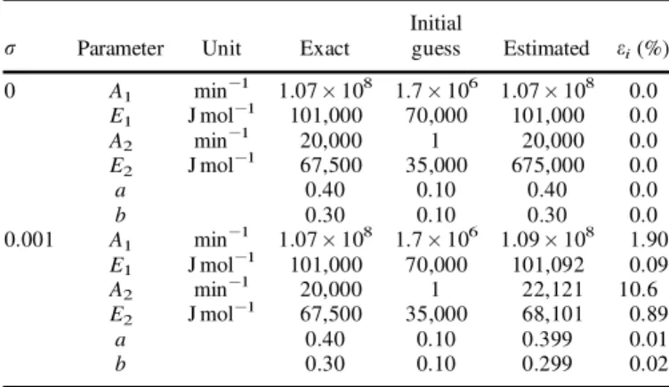
Table 1 summarizes the results obtained for the simulta-neously estimation of six parameters. It shows the initial guess of the unknowns, their recovered and exact values, and their estimation error, respectively. Two levels of measurement errors are considered for numerical analysis including s ˆ 0 (errorless) and s ˆ 0.001, which corre-sponds approximately to 0.1% of the maximum of total mass M(t) during the pyrolysis process.
By using the errorless measurements (s ˆ 0), the six parameters are recovered exactly in 47 s of CPU time and the estimated loss weight matches precisely the measured one. We should mention here that, beyond the displayed initial guess, we cannot get convergence of the estimation algorithm. We observe that, except for the parameter E2, the initial guess of the remain parameters is wide enough with respect to their énal values (exact values).
Also, Table 1 shows the estimated parameters when they are obtained with measurements containing random errors according to equation (17). Generally, the estimated para-meters are in good agreement with their exact values. The highest error is observed with parameter A2and this results from its low sensitivity as underlined in the sensitivity analysis section. The estimation error of parameter A1 is relatively high with respect to the noise level added to the exact data in generating the simulated measurements. Also, this can be explained by its low sensitivity, as shown in Figure 1.
Real Test Case
Pyrolysis of cardboard
Experiments were performed using a SETERAM ATG-DSC-111 apparatus. To generate dynamic data, different cycles were realized for which the temperature increased linearly with time and at different rates, b ˆ dT=dt (K min¡1). The upper temperature value was chosen to ensure that pyrolysis process was complete, as mentioned in the sensitivity analysis.
Figure 3 shows the experimental and model predicted mass evolutions versus temperature obtained with the devel-oped algorithm. Small differences can be observed around the curvature of the measured total loss weight and the étting can be considered as acceptable and efécient. Also, Figure 3 displays the residual of the weight loss, i.e.
M (t) ¡ Y(t). The biggest difference is observed over the
temperature domain [600, 700] and the loss mass residual is still less than 2%. The residual is scattered around zero line during the whole experimental temperature change. If the étting was perfect, i.e. the étting matches precisely the mean measured proéle, we would get the measurement errors
Table 1.Exact, and estimated parameters and their respective estimation error for two simulated test cases.
s Parameter Unit Exact Initialguess Estimated ei(%)
0 A1 min¡1 1.07 £ 108 1.7 £ 106 1.07 £ 108 0.0 E1 J mol¡1 101,000 70,000 101,000 0.0 A2 min¡1 20,000 1 20,000 0.0 E2 J mol¡1 67,500 35,000 675,000 0.0 a 0.40 0.10 0.40 0.0 b 0.30 0.10 0.30 0.0 0.001 A1 min¡1 1.07 £ 108 1.7 £ 106 1.09 £ 108 1.90 E1 J mol¡1 101,000 70,000 101,092 0.09 A2 min¡1 20,000 1 22,121 10.6 E2 J mol¡1 67,500 35,000 68,101 0.89 a 0.40 0.10 0.399 0.01 b 0.30 0.10 0.299 0.02
Figure 2.Solution of the direct problem with exact data (s 0) shown in Table 1.
(noise) instead of the model èuctuations. Figure 4 displays the computed total mass vs the total measured mass loss. As mentioned in the residual analysis, the estimation is accep-table since this égure shows approximately a straight line representing the bisection of the principal axis of Figure 4. By using the experimental data of cardboard pyrolysis, the values of estimated parameters are: A1ˆ 1.07 £ 108min¡1, E
1ˆ 101,107J mol¡1, A2ˆ 19,824min¡1,
E2ˆ 67,648 J mol¡1, a ˆ 0.41 and b ˆ 0.32.
These parameters are obtained in less than 50 s CPU time and with the same initial guesses as displayed in Table 1. In comparison with the estimation procedure developed in our previous paper (David et al., 2003) around the function fmins of Matlab software (MATLAB, 1999), where the estimation time takes over 2 h of computing time, the presented method is more than 100 times faster. This tool will be used in the future to facilitate model building. Finally, the results shown were obtained with a personal computer powered by an Intel1 Pentium 4 processor of 2 GHz, and using 256 MB of RAM, under the Fortran Powerstation platform.
CONCLUDING REMARKS
A numerical procedure is presented for the simultaneous estimation of kinetic parameters characterizing the pyrolysis process of cardboard. The minimization procedure is conducted by minimizing the square difference between experimental measured total mass and the corresponding calculated values from a mathematical model.
A comparison between recovered and exact data showed good agreement. The obtained results underline the robust-ness of the algorithm and its capabilities to recover simulta-neously the kinetic parameters using less a priori information and wide deviation in the initial guess of parameters. This tool is developed by taking into considera-tion some physical constraints such as positiveness of kinetic parameters, and continuity of reaction schemes.
Despite a relatively wide deviation in the initial guess of parameters to be recovered, the presented tool is still sensitive to the initial values. This deéciency is due to the strong non-linearity of the kinetic reacting schemes. Efforts are currently underway to address this problem by consider-ing the genetic algorithms in obtainconsider-ing the best initial guess. Also, the direct estimation of the Arrhenius functions instead of Arrhenius parameters will be analysed by means of function estimation tools.
NOMENCLATURE
A1, A2 Arrhenius factor, min 1
b constant
c constant
E1, E2 activation energy, J mol 1
k1, k2 kinetic reaction rate, min 1
M vector of computed mass
M(ti) computed total mass at time ti
m1, m2, m3 mass fraction
N number of measurements
P number of parameters
R universal gas constant, kJ kmol 1K 1
T temperature, K
t time, min
U vector of unknown parameters
ui unknown parameter i
X sensitivity matrix
Xij sensitivity coefécient
Xij relative sensitivity coefécient
Y vector of measured mass
Y(ti) measured mass at time ti
Greek symbols b heating rate e small number m damping parameter V damping matrix REFERENCES
Bard, Y., 1974, Nonlinear Parameter Estimation (Academic Press, New York, USA).
Beck, J. and Arnold, K., 1977, Parameter Estimation in Engineering and
Science(Wiley Interscience, New York, USA).
David, C., Salvador, S., Dirion, J. and Quintard, M., 2003, Determination of a reaction scheme for cardboard thermal degradation using thermal gravimetric analysis, J Anal Appl Pyrol, 67(2): 307–323.
Font, R., Martin-Gullon, I., Esperanza, M. and Fullan, A., 2001, Kinetic law for solids decomposition. Application to thermal degradation of hetero-geneous materials, J Anal Appl Pyrol, 58–59: 703–731.
IMSL, 1987, Library Edition 10.0, User’s Manual, Math=Library (IMSL Houston, TX, USA).
Figure 3.Comparison between the experimental and the computed loss mass evolution. Weight loss residual evolution as temperature function. The heating rate was taken as b 10 K min 1.
Levenberg, K., 1944, A method for the solution of certain non-linear problems in least square, Q Appl Math, 2(2): 164–168.
Marquardt, D.W., 1963, An algorithm for least square estimation of nonlinear parameters, J Soc Ind Appl Math, 11(2): 431–441.
MATLAB, 1999, Library Edition 5.3, User’s Manual (MathWorks Inc., Natick, MA, USA).
More, J., 1978, Numerical Analysis, Lectures Notes in Mathematics, Dold, E.B. and Watson, G. (eds), Vol. 630 (Springer, Berlin, Germany), pp 105– 116.
Opfermann, J., 2000, Kinetic analysis using multivariate non-linear regres-sion. (i) Basic concepts, J Therm Anal Calc, 60: 641–658.
Press, W., Teukolsky, S., Vetterling, W. and Flannery, B., 1992, Numerical
Recipes in Fortran(Cambridge University Press, Cambridge, UK). Roduit, M.M.B. and Baiker, A., 1996, Inèuence of experimental
conditions on the kinetic parameters of gas–solid reactions— parametric sensitivity of thermal analysis, Thermochim Acta, 282=283: 101–119.
ACKNOWLEDGMENT
The authors would like to express their deep acknowledgements to the reviewers for their constructive critic and remarks in improving the quality of this paper.
ADDRESS
Correspondence concerning this paper should be addressed to Dr T. Loulou, Ecole des Mines d’Albi-Carmaux, Laboratoire de Gnie des Procds des Solides diviss, UMR CNRS 2393, 8100 Albi, France.